The convex hull swampland distance conjecture and bounds on non-geodesics
←
→
Page content transcription
If your browser does not render page correctly, please read the page content below
Published for SISSA by       Springer
                                                                   Received: December 15, 2020
                                                                   Accepted: February 17, 2021
                                                                    Published: March 31, 2021

The convex hull swampland distance conjecture and
bounds on non-geodesics

                                                                                                 JHEP03(2021)299
José Calderón-Infante,a Angel M. Urangaa and Irene Valenzuelab
a
  Instituto de Física Teórica IFT-UAM/CSIC,
  C/Nicolás Cabrera 13-15, 28049 Madrid, Spain
b
  Jefferson Physical Laboratory, Harvard University,
  Cambridge, MA 02138, U.S.A.
    E-mail: j.calderon.infante@csic.es, angel.uranga@csic.es,
    ivalenzuela@g.harvard.edu

Abstract: The Swampland Distance Conjecture (SDC) restricts the geodesic distances
that scalars can traverse in effective field theories as they approach points at infinite dis-
tance in moduli space. We propose that, when applied to the subset of light fields in
effective theories with scalar potentials, the SDC restricts the amount of non-geodesicity
allowed for trajectories along valleys of the potential. This is necessary to ensure consis-
tency of the SDC as a valid swampland criterion at any energy scale across the RG flow.
We provide a simple description of this effect in moduli space of hyperbolic space type, and
products thereof, and obtain critical trajectories which lead to maximum non-geodesicity
compatible with the SDC. We recover and generalize these results by expressing the SDC as
a new Convex Hull constraint on trajectories, characterizing towers by their scalar charge
to mass ratio in analogy to the Scalar Weak Gravity Conjecture. We show that recent
results on the asymptotic scalar potential of flux compatifications near infinity in mod-
uli space precisely realize these critical amounts of non-geodesicity. Our results suggest
that string theory flux compactifications lead to the most generic potentials allowing for
maximum non-geodesicity of the potential valleys while respecting the SDC along them.

Keywords: Flux compactifications, Superstring Vacua

ArXiv ePrint: 2012.00034

Open Access, c The Authors.
                                                       https://doi.org/10.1007/JHEP03(2021)299
Article funded by SCOAP3 .
Contents

1 Introduction                                                                              1

2 Non-geodesic bounds in the hyperbolic plane                                               4
  2.1 One hyperbolic plane                                                                  4
  2.2 Product of hyperbolic planes                                                          7

3 A geometric formulation of the SDC                                                        9

                                                                                                 JHEP03(2021)299
  3.1 Geometric formulation                                                                10
  3.2 Non-geodesic bounds                                                                  12

4 The convex hull SDC                                                                      14
  4.1 General formulation                                                                  14
  4.2 Examples                                                                             17
      4.2.1 The hyperbolic plane complex scalar revisited                                  17
      4.2.2 Two saxions                                                                    18
      4.2.3 Decoupled saxion-axion                                                         20

5 Constraints on the potential and asymptotic flux compactifications                       22

6 Conclusions                                                                              25

1   Introduction

Since the pioneering work in [1–3] and its revival [4–10], recent years have witnessed an
enormous progress in the swampland program, see [11, 12] for reviews. The swampland
program seeks to constrain properties of effective field theories required to be consistently
realizable in theories of quantum gravity (such as string theory). A class of constraints
refers to the properties of the moduli space of massless scalars in the theory, in particular
the Swampland Distance Conjecture (SDC). A loose formulation of its best established
variant [2] is that, as one moves toward infinity in moduli space, there appears an infinite
tower of states with masses going to zero exponentially with the traversed distance, hence
below the cutoff of the effective theory, which thus breaks down. The strong version of this
SDC is that the critical distance controlling this exponential scaling is Planckian [13].
     The SDC has been extensively tested in string theory compactifications [14–29]. Other
discussions of this conjecture involve towers of objects other than particles [30, 31], string
RG flows [32], backgrounds with Anti de Sitter spacetimes [33–36], etc. The central role of
the SDC is also made clear by its connection with other conjectures, like the Weak Gravity
Conjecture [14, 16, 28, 32, 37], the de Sitter conjectures [38–41], the Zk Weak Coupling
Conjecture [42], the emergence proposal [14, 43], etc.

                                            –1–
An important point in the discussion of SDC is that it should apply to adiabatic motion
in moduli space. Morally, this amounts to varying the scalar values as vevs, i.e. with no
spacetime variation. In fact, as shown in [33], backgrounds with spacetime varying scalars
can lead to transplanckian motion without encountering exponentially falling towers of
states.1 A useful way to understand this point is that adiabatic motion corresponds to
moving along geodesics in moduli space, while spacetime dependence introduces extra
forces in moduli space motion, leading to non-geodesic trajectories. This would seem to
imply that the SDC, in the adiabatic sense, should apply only to geodesic trajectories in
moduli space.
On the other hand, although the SDC and its variants are most precisely stated and
JHEP03(2021)299
studied for exactly massless moduli, on physical grounds they should be expected to hold in
the presence of scalar potentials, as long as the relevant masses and energies remain smaller
than the cutoff, i.e. a pseudomoduli space. From this perspective, consider a theory with
a moduli space M parametrized by a set of scalars φi , such that the SDC is satisfied. If a
potential V (φ) is now introduced, the motion of scalars is restricted to the valleys of this
potential, which can either correspond to left-over massless moduli, or to directions along
which the potential may not be exactly flat but the relevant energies are smaller than a
given cutoff Λ. Let us denote this (pseudo)moduli space M. At energies below Λ, we may
integrate out the heavy directions of M and obtain and effective theory for the light scalars
ϕa parametrizing M .
Now this leads to the following conundrum. In the effective theory below Λ, one can
study the SDC by considering geodesic trajectories in the moduli space M. On the other
hand, the trajectory can be regarded as uplifted to a trajectory in M, so that distances
along it can be computed as in the parent theory.2 But these trajectories in general do not
correspond to geodesics in M, and could in principle violate the SDC, even if the SDC is
obeyed for geodesics in M !
A most relevant aspect of this apparent puzzle is that, if actually realized, the SDC
would cease to make sense as a swampland constraint. Given an effective theory violating
the SDC in its moduli space, one could always argue that this corresponds to the theory
on M, and that above certain scale Λ the theory is completed to a larger moduli space M
which obeys it, and which can in principle be completed into a quantum gravity theory.
In fact, there is no reason why this cannot occur in a nested manner with several effective
theories scalating up to some higher energy scale at which finally the SDC is fulfilled. In
other words, since the notion of moduli scape in the presence of multi-scale potentials is a
scale-dependent notion, the SDC constraint would only apply in a certain energy regime,
but then, which energy regime?
We have guided the reader through this argument to make our main point manifest.
We propose that the above situation cannot occur in a theory of quantum gravity, and that
1
For spacetime dependence and transplanckian scalar travel, see also [13, 44, 45].
2
An important point is that the kinetic terms on the effective theory in M are affected by the integration
of the heavy modes; this is captured by the statement that in the effective theory below Λ, the metric on
M is the induced metric from the embedding of M ⊂ M. This is equivalent to the statement that the
distance is obtained from the trajectory when embedded in M.
–2–the SDC must apply at any energy scale, namely, in any of the effective theories valid at
any intermediate energy scale. This has the following profound implication: since arbitrary
scalar potentials in a moduli space M can easily lead to subspaces M violating the SDC,
the validity of the SDC at all scales in quantum gravity theories constitutes a non-trivial
constraint on consistent potentials in quantum gravity theories.
The realization of the SDC in moduli spaces of light fields in the presence of potentials 3
has been explored in diverse examples in flux compactifications in string theory e.g. [48–
50]. These top-down approaches are valuable, yet very model dependent. In this paper we
instead initiate a model-independent bottom-up approach, closer to the spirit of the swamp-
land program. Our strategy is instead to characterize the non-geodesic trajectories which
JHEP03(2021)299
are nevertheless ‘sufficiently geodesic’ to allow the realization of the SDC. The approach is
very model independent, since it only involves geometrical properties of the moduli space,
and some information about the towers hiding at its asymptotic regions. Characterization
of the non-geodesicity allowed by the SDC for trajectories in a moduli space, leads in in-
teresting examples to explicit bounds. These bounds can be subsequently tested against
concrete models, and are interestingly saturated in string theory flux compactification in
the asymptotic limits [51].
The model-independent approach allows us to devise an illuminating rephrasing of
the SCD in terms of a Convex Hull condition, similar in spirit to that arising in the
context of the Weak Gravity Conjecture [52], or its scalar WGC (SWGC) extensions [53–
58]. In particular, we characterize SDC towers by a scalar charge to mass ratio as in the
SWGC; this controls the exponential decay rate along asymptotic trajectories characterized
in terms of their asymptotic unit tangent vectors. Conversely, by considering the space
of such vectors for all possible trajectories, we define an ‘extremal region’ by the set of
charge to mass ratios ensuring a fixed minimum decay rate along any possible trajectory.
Although in the original formulation of the SDC [2], the decay rate is an undetermined
O(1) factor, concrete lower bounds have been proposed in [14, 28, 32, 39–41]. This allows
to express the SDC in a given physical system as the condition that the convex hull of the
scalar mass to charge ratios of its towers contains the extremal region. If the convex hull
condition is not satisfied for arbitrary trajectories, one can use the convex hull to recover
the above mentioned bounds on the non-geodesicity of the trajectories. Alternatively, it
can also be used to predict the existence of new towers.
The fact that the scalar charge to mass ratio in our Convex Hull SDC agrees with
the SWGC is a tantalizing hint, although the physical requirement of ‘extremality’ in both
situations does not seem to be necessarily identical. It would be interesting to explore the
relationship between the WGC states and the SDC towers in this Convex Hull context,
possibly along the lines of [16, 28].
The paper is organized as follows. In section 2 we consider the example of non-geodesic
trajectories in a moduli space given by one hyperbolic plane (section 2.1) or products thereof
(section 2.2), and derive bounds on the non-geodesicity of trajectories obeying the SDC.
3
In the original work [2] (see also [46, 47]), it was already noted that the SDC also applies to the
subspaces parametrizing minimum loci for the potential for a given effective cutoff scale, and that this can
imply powerful constraints on the potentials consistent with QG.
–3–The analysis of the multi-moduli cases motivates section 3, where we frame the multi-axion
examples in a general reformulation of the SDC (section 3). This allows us in section 4 to
formulate our Convex Hull SDC (section 4.1), and recover and vastly generalize results of
the previous sections, as we show in several explicit examples (section 4.2). In section 5
we revisit the results about asymptotic flux compactifications in [51], and show that they
realize the critical behaviours of non-geodesicity. Section 6 contains our final remarks.
2 Non-geodesic bounds in the hyperbolic plane
We focus our analysis on trajectories approaching points at infinity in moduli space, in
JHEP03(2021)299
the spirit of the SDC, since the interesting physics occurs in the asymptotic region near
infinity. Also, it often corresponds to weakly coupled regimes, where effective actions and
scalar potentials can be reliably computed. Moreover, fairly general moduli spaces simplify
in the asymptotic regime, so that very simple moduli space geometries are useful templates
for the asymptotics of general moduli spaces.
In this section, we discuss moduli spaces given by a hyperbolic plane, or products
thereof. Despite their apparent simplicity, they are key to describing moduli spaces of
general CY compactifications near their boundaries at infinity [14, 17, 51], to the extent
of encoding much of the dynamics of these models [59]. Moreover, they allow for explicit
computations which will be useful to motivate our generalizations in later sections.
2.1 One hyperbolic plane
Consider a 4d effective theory with two real moduli s and φ with kinetic terms
n2
( ∂µ s ∂ µ s + ∂µ φ ∂ µ φ ) , (2.1)
s2
where n is a free parameter. In other words, the moduli space M is given by the upper
half-plane with metric
n2
d∆2 = 2 ds2 + dφ2 . (2.2)
s
We note that n determines the Ricci scalar curvature
2
R=− . (2.3)
n2
This geometry is ubiquitous in string theory, with φ corresponding to some periodic axion
and s its ‘saxion’ partner (although we do not assume susy, we stick to this name). For
instance, the type IIB complex coupling in 10d, the 4d axio-dilaton in string compactifica-
tions, and the Kähler and complex structure moduli of 2-tori in toroidal (and orbifold and
orientifolds thereof) compactifications.
In many of these, the SL(2, R) symmetry of the above geometry lead to an exact infin-
ity discrete SL(2, Z) duality symmetry. However, we work in a more general perspective, so
that our analysis is valid in the absence of this symmetry. On one hand, in many compact-
ifications, we would like to regard the above metric as a good approximation to the moduli
space (or suitable subspaces thereof) of CY compactifications, in the large s asymptotic
–4–region; hence the region near s = 0 is not relevant to this physics context, and the duality
s → 0 and s → ∞ is a mere artifact. Second, the discrete axion periodicity (which would be
present even near s → ∞) is in general spontaneously broken in the presence of potentials
of axion monodromy4 kind [60, 61], a generic situation in flux compactifications [62, 63].
Hence we consider φ to take real values, with no identification whatsoever.
We consider that the SDC is satisfied on this moduli space M, namely there exists a
tower of states with mass scale5
M ∼ s−a , a > 0. (2.4)
If s parametrizes the vertical axis, all geodesics in this space are either vertical lines
JHEP03(2021)299
or half-circles with centers on the s = 0 line. Thus, the only geodesics approaching s → ∞
are vertical lines with φ = const. For these geodesics, the distance behaves as
∆ ∼ n log s (2.5)
(with n taken positive herefrom). The mass scale of the tower reads
a
M ∼ exp − ∆ ∼ exp (−α∆) , (2.6)
n
thus leading to the SDC with decay rate α = na . This is indeed O (1) in many realizations
in string theory.
Let us now consider a general trajectory approaching s → ∞ in this moduli space. For
reasonable trajectories, we can use s to parametrize it,6 so that the curve is defined by the
expression
φ = f (s) (2.7)
for some function f that we assume sufficiently smooth. This is a template to describe the
moduli space of an effective theory in which there is partial moduli stabilization, and the
light direction can be parametrized by s.
Recalling footnote 2, note that the distance in this effective theory is not measured by
just the metric component gss , but rather by the effective metric obtained upon replacing
the s-dependent value of φ in the underlying metric. This is equivalent to measuring
distance along the trajectory with the ambient space metric (2.2) in M. This yields
n
q
d∆ = 1 + f 0 (s)2 ds. (2.8)
s
4
More precisely, the discrete periodicity is preserved due to the multiple-branched structure of the
potential. However, it is spontaneously broken when the problem under study (e.g. adiabatic motion in
moduli space) is restricted to a single branch.
5
The fact that the overall scale is independent of φ does not imply that the masses of individual states
in the tower can not depend on φ. Indeed, a typical structure is given by Mn = M |n + φ|, with n labeling
states in the tower and M depending only on s, as required for our analysis. Here the φ-dependence is
determined by the fact [14, 18] that the different states in the tower are generated by monodromy in φ, i.e.
φ → φ + 1 is equivalent to n → n + 1. More general axion dependences in the tower scale will be easily
included in the analysis in section 4.
6
Actually, requiring that the trajectory eventually goes to s → ∞ makes this parametrization always
valid for sufficiently large s.
–5–We can now classify general trajectories in three different kinds, according to the
asymptotic behaviour of f 0 (s) in the s → ∞ limit:
• The Asymptotically Geodesic case: this corresponds to f 0 (s) → 0, and we have
ds
d∆ = n . (2.9)
s
Trajectories of this class approach a geodesic when s → ∞. Therefore the SDC is
automatically satisfied with decay rate
a
αgeod. = (2.10)
JHEP03(2021)299
.
n
• The Critical case: this corresponds to f 0 (s) → β = const. and we have
q
ds
d∆ = 1 + β2 n . (2.11)
s
The tower of states has mass scale
!
α
M ∼ exp − p ∆ , (2.12)
1 + β2
which is consistent with the SDC, but modifies the scale of the exponential. We can
define a factor
αgeod
ν≡ (2.13)
αnon-geod
αgeod
that measures such a modification, so that M ∼ exp(− ν ∆). In this case we have
q
a
νcrit. = 1 + β 2 → αcrit = p . (2.14)
n 1 + β2
Hence, ν → ∞ corresponds to a violation of the SDC in a non-geodesic trajectory.
• The Swampy case: this corresponds to f 0 (s) → ∞, and we have
|f 0 (s)|
d∆ = n ds . (2.15)
s
Here we can evaluate the behaviour of the tower by computing
d log M d log M ds a −1
= = − f 0 (s) → 0. (2.16)
d∆ ds d∆ n
This violates the SDC since the tower mass scale is no longer falling exponentially
with the distance.
We note that the critical case corresponds to the maximum deviation from a geodesic
still consistent with the SDC. It therefore provides a non-trivial bound that any light
direction in the moduli space (after partial moduli stabilization by some scalar potential)
must obey. Notice that this is the class of curves in which the saxion varies linearly with the
–6–axion (s ∼ a). This will be contrasted with explicit string models of flux compactifications
in section 5, where we show that this class of models saturates the bound.
It is interesting to explore the characterization of these classes in terms of a geometrical
quantity of the trajectories. A natural scalar measure of non-geodesicity is the modulus
|Ω| of the proper acceleration7
Ωi = T j ∇ j T i , (2.17)
where T is the normalized tangent vector of the trajectory and ∇ is de covariant derivative
in moduli space. In our case we have
JHEP03(2021)299
2
f 0 (s) + f 0 (s)3 − sf 00 (s)
|Ω| =
2
. (2.18)
n2 (1 + f 0 (s)2 )3
We can now characterize the three classes of paths above in terms of the asymptotic
behaviour for |Ω| as follows. The Asymptotically Geodesic case corresponds to f 0 (s) → 0
which translates to |Ω|2 → 0 . The proper acceleration vanishes asymptotically, since the
trajectory approaches a geodesic. Contrary, for the Swampy case, one has f 0 (s) → ∞
leading8 to |Ω|2 → n12 . Thus, the proper acceleration at s → ∞ attains a maximal value,
and signals a hard violation to the SDC. Finally, the Critical case corresponds to
1 β2
f 0 (s) → β = const. =⇒ |Ω|2 → . (2.19)
n2 1 + β 2
The change in the parameter of the exponential defined in (2.13) can be written as
1
ν=p . (2.20)
1 − n2 |Ω|2
We can thus recast the criterion that the trajectory respects the SDC as a bound on the
non-geodesicity:
|R| 1
|Ω|2 < = 2 (2.21)
2 n
In the next subsection, we will generalize these bounds to higher dimensional moduli
spaces in which there is more than one hyperbolic plane. We will see that they cannot
be stated simply in terms of the modulus of the proper acceleration, as the direction will
also matter. In other words, the bounds will vary depending on the type of trajectory/ the
growth sector to which the trajectory belongs.
2.2 Product of hyperbolic planes
We now consider a moduli space given by a product of hyperbolic planes. For simplicity,
we consider the case of two, which suffices to illustrate the point. The metric is
n2 2 m2
d∆2 = 2
ds + dφ2 + 2 du2 + dψ 2 . (2.22)
s u
7
Actually, since our trajectories are not worldlines, we should use the term “extrinsic curvature”, but
we stick to the kinematical language.
00 n
8
One also needs that sff 03
→ 0. This is satisfied for all functions of the form f (s) = sn , (log s)n , es .
–7–As in section 2.1, we focus in paths approaching the infinite distance regime s, u → ∞.
Note that this setup (2.22) nicely models the asymptotic behaviour of CY moduli spaces,
cf. section 5, thus our discussion is of direct relevance to the study of non-geodesic paths
in CY moduli space.
In order to satisfy the SDC for geodesics, it is enough to introduce a tower of states
for each of the hyperbolic planes, with mass scales
Ms ∼ s−a , Mu ∼ u−b , a, b > 0. (2.23)
It is clear that these towers enforce the SDC for geodesic paths contained in a single
JHEP03(2021)299
hyperbolic plane. Moreover, one can show that they also suffice to recover the SDC for
more general geodesics.9
Let us consider non-geodesic paths approaching infinity in different ways, some of
which correspond to different growth sectors, in the terminology of [17]. For instance, we
can consider paths that only move on one of the hyperbolic planes, namely approaching
s → ∞ while keeping u, φ fixed, or alternatively, approaching u → ∞ with s, φ fixed. In
that case, the situation is equivalent to the one discussed in section 2.1 and we can simply
borrow the classification of asymptotically geodesic, critical and swampy trajectories. We
could also apply the criterion (2.21) on the proper acceleration |Ω|2 , although this would
yield two different bounds for the two different curvature paratemeters n and m. In other
words, there is no single discriminating criterion on |Ω| which applies to both kinds of
paths.
On the other hand, we may consider a path
ψ = f (s) with φ, u const. (2.24)
so that we move along a trajectory involving the axion and saxion of different hyperbolic
planes. The distance along this curve is given by
s s
n 2 m2 0 2 n m2 s 2 0 2
d∆ = 2
+ 2 f (s) ds = 1+ f (s) ds . (2.25)
s u s n2 u 2
In the second equality we recognize the two terms in the square root to be the geodesic
and the non-geodesic contribution to the field distance.
As done in section 2.1, we can classify the trajectories in the same three different
families, depending on the relevance of the non-geodesic contribution in the asymptotic
limit s → ∞. We thus see that the critical case is:
m2 s2 0 2
f (s) → const. , (2.26)
n2 u 2
which means that sf 0 → γ = const., implying the critical behaviour
f (s) → γ log s . (2.27)
9
Physical realizations like CY compactification may produce additional towers. This is ignored in this
section for simplicity, but is included in the general analysis in later sections.
–8–If f (s) grows slower or faster than this critical case one gets the asymptotically geodesic
and the swampy case respectively.
The SDC will only be satisfied for asymptotically geodesic or critical trajectories. Only
for those paths, the towers of states in (2.23) will still exhibit the exponential behaviour
in terms of the distance along the path. Recall that the critical case is the maximum
deviation from a geodesic still consistent with the exponential behaviour required by the
SDC, although the factor in the exponential changes. For a tower with Ms ∼ s−a one finds
α
Ms ∼ exp − , (2.28)
ν
JHEP03(2021)299
with α = a
n being the geodesic decay rate, and the factor of violation of the SDC given by
s
m2 γ 2
ν= 1+ . (2.29)
n2 u 2
In comparison with the case of dual axion-saxion pair, we find that this factor varies when
choosing different u = const. planes.
This also produces a direct relation, albeit a different one, between ν and the modulus
of the proper acceleration. Indeed we find
1
ν=p . (2.30)
1 − m|Ω|
Hence the existence of two axionic directions on which the path can wind lead to
different relations between ν and |Ω|. An implication is that, taking the ν → ∞ limit, they
lead to different discriminating criteria. The critical values correspond to |Ω| → n1 and
|Ω| → m 1
, when moving along φ or ψ respectively.
The difficulty in finding a criterion based solely on the modulus of the proper acceler-
ation is that |Ω| misses the information about the direction in moduli space. And trying
to include this information more explicitly may quickly run into nasty and unphysical de-
pendences on the coordinates chosen in moduli space. In the next section we provide a
concrete description which avoids these pitfalls, and yet allows to provide a purely geo-
metrical reformulation of the SDC in general moduli spaces. We will then translate this
general criterion into a Convex Hull SDC condition in section 4.
3 A geometric formulation of the SDC
Let us recap our approach in general language. Consider some theory satisfying the SDC,
i.e. containing towers of states decaying exponentially for every geodesic approaching an
infinite distance limit of the moduli space M. When adding a scalar potential lifting some
of the directions, we will be left with a new moduli space M whose geodesic trajectories
might lift to non-geodesic trajectories in M. To satisfy the SDC in the new IR theory, we
need that the level of non-geodesicity of these trajectories is small enough to still allow for
exponentially falling towers. Given the field metric of M and the towers of states, we can
always identify the non-geodesic trajectories that are consistent with satisfying the SDC
–9–in the IR theory, where the limiting cases are dubbed critical paths. This was done in
section 2 for the case of products of hyperbolic planes, obtaining specific bounds for the
critical paths. However, this procedure requires specific information about the geometry
of the moduli space, so it needs to be worked out case by case.
In this section, we are going to take a step back and reformulate the SDC in a language
that will allow us to generalise the results of section 2 for general moduli spaces. This will
be later translated into a Convex Hull condition in analogy to the WGC in section 4. The
strategy is to provide a geometric description of the criteria for trajectories to fulfill or
violate the SDC. We will keep the nomenclature introduced in section 2 to distinguish
between the different types of trajectories, namely:
JHEP03(2021)299
• Asymptotically geodesic paths: they approach a geodesic in the asymptotic limit, so
the exponential rate is that of the geodesic.
• Critical paths: non-geodesics that still marginally allow for the exponential decay of
the tower, although the exponential rate differs from the geodesic one.
• Swampy paths: they highly deviate from geodesics so the tower does no longer fall
exponentially.
3.1 Geometric formulation
The general formulation of the SDC establishes that, for any geodesic in moduli space in
an infinite distance limit there exists a tower of states with mass scale
M = exp ( −α ∆ ) (3.1)
with positive α > 0. Stronger versions of the conjecture further require α > O (1), moti-
vated by string theory setups. Let us now focus in the mildest version and simply require
α > 0, leaving the study of the implications of α > O (1) for the next subsection.
Consider a trajectory γ approaching an infinite distance point in moduli space. We
start by rewriting the exponential decay rate α of the tower mass scale as
d log M
α(∆) = − = −T i ∂i log M , (3.2)
d∆
where T is the normalized tangent vector of γ, and M is implicitly evaluated along it.
This rewriting shows that the only information about γ relevant for the SDC is the
limiting tangent vector when approaching the infinite distance point. This agrees with our
observation that the modulus of the proper acceleration (2.17) is not the right quantity to
discriminate the behaviour of asymptotic trajectories.
An important observation is that the set of allowed asymptotic tangent vectors T
near a point at infinity is in general restricted, in particular for asymptotically geodesic
trajectories.10 For instance, in the hyperbolic plane case, any curve approaching s → ∞
with bounded φ must have φ̇ → 0; hence only the asymptotic tangent vector in the s
10
Notice that for this it is crucial that the point at infinity is singular. For a regular point, space is locally
flat and thus any tangent vector corresponds to a geodesic passing through it.
– 10 –direction is allowed. On the other hand, relaxing the asymptotic geodesicity requirement
allows to explore more general vectors T , as in the case of critical or swampy trajectories.
To reflect this fact, we define the subspace G as that spanned by asymptotic tangent vectors
of asymptotically geodesic trajectories.11
Let us now consider the implications of the SDC (in its milder version) for such asymp-
totically geodesic trajectories. We note that what appears in (3.2) is the scalar product
between the (limit) tangent vector and the gradient of log M . This implies that a single
tower of states along an asymptotically geodesic direction suffices to satisfy the SDC for
any other direction, except for the orthogonal ones. Thus, the minimal requirement of the
SDC is that there exist as many towers as orthogonal limit tangent vectors in G.
JHEP03(2021)299
Actually, in general, there may exist other towers of states beyond the above minimal
set. Hence it is convenient to consider a new subspace, denoted by M, spanned by the
gradient vectors of (log of) the scale M , for all existing towers of states. Note that in many
string theory realizations the directions associated to such towers are “dense”; for instance,
in a KK compactification on S1 × S1 near the decompactification limit R1 , R2 → ∞, there
are towers of KK states with masses
n 2 n 2
1 2
M2 = + . (3.3)
R1 R2
Hence, for any rational direction of γ i.e. R ≡ R1 /q1 = R2 /q2 , there is a tower of states
with mass M ∼ n/R by taking the states n1 = nq1 , n2 = nq2 .
In terms of these spaces, the mildest version of the SDC (with α > 0) can be ex-
pressed as:
For any vector in G (i.e. any asymptotically geodesic tangent vector),
there must be at least one non-orthogonal vector in M (i.e. a suitable
tower of states becoming massless).
Equivalently, the projection of M onto G should completely fill the latter:
PG M = G . (3.4)
Incidentally, this implies that their dimensions satisfy dim M ≥ dim G.
This geometric formulation of the SDC resembles a kind of Completeness Hypothesis
where the towers of states play the role of the charge spectra in gauge field theories.
Analogously, here the role of the charge space is played by the space of asymptotic tangent
vectors of asymptotically geodesic trajectories. Stronger conditions - similar to the WGC -
will appear when further requiring the towers to satisfy a lower bound for the exponential
rate α ≥ α0 , with α0 some order one constant. This mild formulation, though, already
allows us to extract interesting conclusions. The first observation is that a single tower
of states might not suffice to satisfy the SDC whenever the space G is spanned by more
than one tangent vector while M remains one-dimensional. This can occur e.g. in higher
11
Strictly speaking, we are interested in the subset containing all asymptotically geodesic vectors, which
may not necessarily form a vector subspace. However, being it the case in all the examples at hand motivated
by string theory, we will treat G as a well-defined vector subspace.
– 11 –dimensional moduli spaces in which the tower misses to depend on at least one of the
saxions. A second observation is that, by satisfying the above criterion, we are actually
fulfilling the SDC along a more general set of trajectories beyond geodesics. We will
characterize this set of trajectories in the next subsection.
3.2 Non-geodesic bounds
We can now turn to characterizing which trajectories could satisfy or violate the SDC.
Indeed, the presence of a single tower makes the mild version of the SDC satisfied for all
its non-orthogonal directions, and not only geodesics. Taking into account all possible
JHEP03(2021)299
towers, this defines a subset TSDC composed by all the directions that satisfy the SDC. In
this way, the SDC can be reformulated as imposing that this subset must contain all the
asymptotically geodesic directions,
G ⊂ TSDC . (3.5)
Clearly, swampy trajectories violating the SDC will therefore correspond to those not
belonging to TSDC . Notice that, for this mild version, TSDC is just the whole set of directions
in moduli space minus the orthogonal complementary of the subspace M. Hence, critical
trajectories also belong to TSDC in this mild formulation.
Let us now turn to the stronger version of the SDC, in which we impose a lower
bound for the exponential rate α ≥ α0 with α0 some O(1) constant. It is reasonable
to assume that α cannot take arbitrarily small values as otherwise it would violate the
exponential behaviour required by the SDC. Moreover, all string theory examples studied
so far have O(10−1 − 10), and precise bounds have been given in the context of towers of
BPS particles in Calabi-Yau compactifications [14, 28]. There, one finds that α ≥ √12n for
a CYn , implying α ≥ √16 for a CY3 Type II compactification to four dimensions. A lower
bound has also been motivated by using the Transplanckian Censorship Conjecture [39–
41] or by identifying infinite distance limits with RG flow endpoints of BPS strings in 4d
N = 1 EFTs [32]. Here, we will not commit to any of these specific values for α0 although
it would be extremely interesting to get a better understanding of this.
We can now extend the last formulation in (3.5) to include the lower bound on α
by finding an appropriate definition of TSDC . To do this, let us recast the scalar product
in (3.2) in terms of the angle θ between the (limit) tangent vector and the gradient of
log M , and get
α = −|∂ log M | cos θ . (3.6)
Here we see that a single tower will make the SDC with α ≥ α0 satisfied for any direction
such that
α0
cos θ ≤ − . (3.7)
|∂ log M |
This is, each tower will then come with an associate cone of directions satisfying the SDC,
CM (α0 ), and defined by (3.7). Therefore, TSDC will be formed by the union of the associate
cones of all the towers of states (see figure 1), this is,
TSDC = CMi (α0 ) . (3.8)
[
– 12 –JHEP03(2021)299
Figure 1. Pictorial representation of the subset of directions TSDC . There are two towers of states
and their associated cones are represented. Every direction outside both of these cones does violate
the SDC for α ≥ α0 .
With this definition, the SDC with α ≥ α0 reduces again to (3.5). Notice that not all
critical trajectories will satisfy (3.7), so only a subset of them will belong to TSDC , whose
definition now depends on α0 . We will translate this condition into a convex hull condition
in section 4, which provides an equivalent but simplified and more elegant formulation of
the above criterion.
In general, determining TSDC is not only associated to the non-geodesicity of the tra-
jectory but requires full information about the tower of states. However, it becomes a
purely geometric condition in the particular case that
M = G. (3.9)
In this situation, the realization of the SDC is such that the non-geodesicity of trajectories
is directly related to the slow-down of the exponential falloff of state masses along them.
It is in this case when the moduli space geometry completely determines the structure of
the towers near infinity, as indeed occurred in earlier examples, and in most string theory
examples. Hence, it is a natural framework to discriminate the asymptotically geodesic,
critical and swampy trajectories, generalizing our discussion in section 2.
Our approach allows to go even further, and also obtain the modification factor ν in
the exponential decay rate for the non-geodesic cases, as follows. The exponential rate
in (3.2) can be written as
α = −(PM T )i ∂i log M = −(PG T )i ∂i log M . (3.10)
where we have used (3.9) in the last step. Notice that PM T is nothing else than cos(θ)
defined in (3.6). For a unit vector in G, the result of this expression is the non-vanishing
exponential decay rate required to fulfil the SDC along geodesics, i.e.
α = |PG T | αgeod . (3.11)
– 13 –Hence, the factor ν in (2.13) is given by
ν = |PG T |−1 = (1 − |PG⊥ T |2 )−1/2 . (3.12)
It is straightforward to apply these concepts to recover the results for the hyperbolic
space in section 2.1. As can be readily checked from (2.4), the relevant subspaces are
spanned by ∂s ,
G = M = h ∂s i . (3.13)
For trajectories φ = f (s) we have the tangent vector
JHEP03(2021)299
s
T = p ∂s + f 0 (s) ∂φ . (3.14)
n 1 + f (s)
0 2
Non-geodesic trajectories are those with a nontrivial ∂φ component in their limit tangent
vector. Finally, the criterion depending on the modulus of the proper acceleration (2.20)
is recovered from (3.12) by checking, in the limit s → ∞, the relation
PG⊥ T = n|Ω|. (3.15)
One can similarly recover the results for products of hyperbolic spaces from these
considerations, as the interested reader in encouraged to check. We instead move on to
provide an even more intuitive formulation of these criteria in terms of a Convex Hull
condition similar to that used for WGC.
4 The convex hull SDC
In this section we formulate the SDC in terms of a Convex Hull condition in the space of
asymptotic trajectories. This will let us to easily recover our earlier results about different
classes of asymptotic trajectories in a pictorial way which is more familiar in the Swampland
program. Moreover, it will also allow us to generalize the story for any combination of
towers of states and any asymptotic structure of the field space.
4.1 General formulation
Consider a trajectory γ approaching an infinite distance point in moduli space and T~
its normalised tangent vector. As in section 3, we denote by G the subspace spanned
only by asymptotically geodesic vectors, i.e. that approach a geodesic trajectory at infinite
distance. We have seen that requiring the existence of an infinite tower of states becoming
light along any of these asymptotically geodesic trajectories, actually allows for satisfying
the SDC along a more general set of trajectories characterised by vectors in TSDC ⊃ G.
This larger space allows for a certain level of non-geodesicity, including critical paths but
excluding swampy trajectories, according to the nomenclature summarised at the beginning
of section 3. If we require a stronger version of the SDC in which the exponential rate
in (3.2) satisfies a lower bound α ≥ α0 , only a subset of the critical paths will be included
in TSDC . In other words, the SDC with α ≥ α0 is equivalent to requiring that, for any
– 14 –direction in G, there must exist a tower of states such that the gradient vector of log M
projected onto that direction is sufficiently large. Our goal now is to translate this statement
into a convex hull condition.
The key observation is that there is a formal analogy with WGC quantities. The
gradient of M can be regarded as the scalar charge of the tower under the moduli. We
can also think of G as the vector space of possible ‘charge’ directions. Hence, the previous
criterion can be rephrased as requiring that for every charge direction, there must exist a
charged infinite tower of states satisfying α(∆) ≥ α0 asymptotically, where α0 is a fixed
contant (of order 1) which quantifies the criterion of fast enough decay to satisfy the SDC.
The SDC conditions can thus be formulated in analogy with the scalar version of the
JHEP03(2021)299
WGC [53]. In particular for a tower with (scalar dependent) mass scale M , we can define
a scalar charge to mass ratio
1
~z = −g − 2 ∇
~ log M , (4.1)
where g 1/2 is a matrix whose square is the field metric (more precisely, introducing the
n-vein eai ebj δab = gij , we have z a = −eai g ij ∂j log M ). The inclusion of the metric absorbs a
piece in (3.2), such that scalar products become cartesian in the following.
The scalar WGC requires the existence of at least one state satisfying |~z| ≥ O(1), such
that the gravitational force acts weaker than the scalar force [53] (see [58] for a different
motivation of this proposal). Hence, the order one factor is typically fixed such that states
saturating the scalar WGC should feel no force. Unlike with the usual WGC, the order
one factor is not associated to extremality of black holes but, for convenience, we will keep
the terminology extremal to refer to those states saturating the bound. At first glance, it
seems that the scalar WGC is different to the SDC, as for the latter what matters is not the
modulus of the scalar charge to mass ratio but the projection over a trajectory. However,
we will se that the SDC can actually be understood as a Convex hull Scalar WGC in which
the extremal states are instead identified as those decaying exponentially with a minimum
rate α0 .
Consider a vector space of dimension equal to the number of scalars under consider-
ation, and a general unit vector ~n therein to parametrize the asymptotic behaviour of a
general trajectory. This is related to the earlier vector T~ by na = eai T i , and is unit norm
with respect to the Cartesian dot product. We define the extremal states as those with a
scalar charge to mass ratio vectors ~z satisfyng
~n · ~z = α0 (4.2)
for some fixed α0 > 0 determining the lower bound for the SDC exponent. From (3.2), we
see that for fixed ~n, this corresponds to the full set of towers with exponential rate α0 along
the asymptotic trajectory defined by ~n. It corresponds to a hyperplane orthogonal to ~n,
at a distance α0 from the origin. Scanning over all possible unit vectors,12 we define the
12
Note that we allow for both positive and negative values of all components of ~n. This is unphysical
for the scalars becoming large in trajectories going off to points at infinity. However, we allow for this
possibility at the formal level, to produce a simpler formulation of the convex hull condition, out of which
the physical constraints follow from simple restriction of the allowed trajectories.
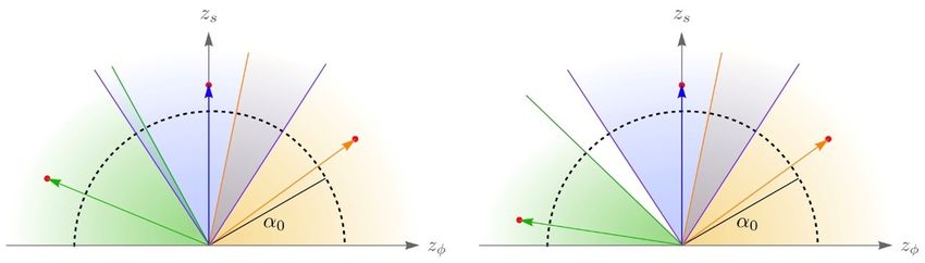
– 15 –JHEP03(2021)299
Figure 2. The extremal region as envelope of hyperplanes.
extremal region as the enveloping hypersurface defined by the set of all such hyperplanes.
It corresponds to a sphere or radius α0 , see figure 2.
By allowing the sphere in figure 2 to take any radius, we recover the mildest version of
the SDC in which α is an undetermined positive constant, α > 0. However, it seems reason-
able to consider a finite radius for the extremal ball which cannot be taken parametrically
small, as that would spoil the exponential behaviour and violate the SDC. Determining
how small α can get is one of the biggest open questions of the SDC and, as explained
above, specific lower bounds have been proposed in the literature [14, 28, 32, 39–41]. One
possibility motivated by the key role of the scalar charge to mass ratio above is that α0
can indeed be determined by using the scalar WGC or some sort of no-force requirement,
as it was probably envisioned in [53]. This would be very interesting as it might be used
to provide a bottom-up rationale for the SDC.
It is now straightforward to define the SDC in terms of a convex hull13 condition:
Convex hull SDC: in a theory with a set of towers corresponding to
scalar charge to mass ratios ~zi , the requirement that the SDC is satisfied
(with at least decay rate α0 ) by any trajectory is exactly the condition
that the convex hull of the vectors ~zi contains the above defined extremal
region, namely the unit ball of radius α0 .
Alternatively, it is possible that the SDC convex hull condition is not satisfied, so
the SDC does not hold (with decay rate α0 ) for all trajectories, but it still applies to
some trajectories. In this situation we can put bounds on the trajectories not to become
swampy, constraining the level of non-geodesicity allowed such that the SDC is satisfied.
This situation naturally occurs when we start with a UV theory satisfying the SDC and
then add a scalar potential lifting some directions, so we are left with a IR moduli space
13
To achieve a full convex hull, we formally use the method of images and also include the mirror vectors
along the negative directions mentioned in footnote 12.
– 16 –whose geodesics might lift to non-geodesics from the UV perspective. In this case, we can
use the convex hull SDC in the UV theory to constrain the allowed set of non-geodesic
trajectories that would still allow us to comply with the SDC in the IR. The advantage of
this formulation is that it also allows us to incorporate the possibility that new towers of
states appear in the IR theory when adding the scalar potential. Hence, the Convex Hull
SDC can be used to constrain either:
• the spectra of the theory, by requiring as many towers as needed to satisfy the convex
hull condition,
JHEP03(2021)299
• or the possible trajectories along which the SDC can be satisfied for a fixed set of
towers and, therefore, the scalar potentials consistent with quantum gravity.
This latter option is not possible in the usual WGC, as the charge lattice is typically a
fixed input of the theory.14 However, it is very natural in the context of the SDC, as the
allowed set of trajectories consistent with quantum gravity is still an open question, as it
depends in turn on what scalar potentials can be realised in quantum gravity.
4.2 Examples
In this section we illustrate these ideas with examples, reproducing and generalizing the
results in previous sections.
4.2.1 The hyperbolic plane complex scalar revisited
Consider the case of the hyperbolic plane in section 2.1. Using the metric (2.2) the charge
to mass ratio vector for a tower with mass scale M is
s
~z = − (∂φ log M, ∂s log M ) . (4.3)
n
Asymptotically geodesic trajectories have a tangent vector which approaches ~n = (0, 1)
asymptotically. Critical trajectories are parametrised by (2.7) with constant f 0 = β, so the
unit vector is
1
~n = p (β, 1) . (4.4)
1 + β2
For these trajectories the vector ~n is constant so that (4.2) corresponds to the equation of
a straight line in the plane (z1 , z2 ). Different trajectories with different values of f 0 will
give rise to different straight lines, e.g. horizontal lines correspond to a purely saxionic
trajectory, and bigger β leads to bigger slopes.
For the particular case of a single tower M ∼ s−a , cf. (2.4), we have a single point
(and its image) at ~z = (0, ±a/n). Clearly, the convex hull of these two points does not
14
Actually, the charge lattice can vary after higgsing a gauge group. If the higgsing is too large, this can
lead to a violation of the WGC in the IR, even if it was originally satisfied in the UV. This is a known
loophole of the WGC [64]. From our perspective, by analogy with the SDC, the resolution is that the
amount of higgsing should be restricted in quantum gravity, so the WGC could also be used to constrain
the allowed IR charge lattices.
– 17 –JHEP03(2021)299
Figure 3. The bound on almost saxionic trajectories.
contain the ball of radius α0 , hence it does not satisfy the SDC for any trajectory. The
SDC is satisfied only in the purely saxionic (geodesic) direction if a/n > α0 , or trajectories
close enough to it. We can then use the convex hull condition to put a bound of how much
a trajectory can deviate from the geodesic saxionic trajectory. For this porpuse, we just
need to compute the angle cos θ = 1/ 1 + βmax at which a tangent trajectory to the ball
p
2
passes by the point ~z = (0, ±a/n) (see figure 3). This occurs for a trajectory with
2
a
−2
βmax = (cos θ) −1= −1 (4.5)
nα0
Hence, critical trajectories with β ≤ βmax will satisfy the SDC with a exponential rate
given by
a
αcrit. = p , (4.6)
n 1 + β2
recovering the result (2.14) in section 2.1.
Alternatively, if one is interested in enforcing the SDC for any trajectory, we have to
introduce more towers, such that the convex hull of their ~z’s encloses the extremal region.
In figure 4 we depict situations with different towers and fulfilling, or not, the SDC for
any trajectory. It is instructive to compare with the criterion in section 3.1 in terms of the
cones comprising TSDC , see figure 5.
4.2.2 Two saxions
Let us consider now a theory with two saxion-like real scalars, namely with a metric
n21 2 n22 2
d∆2 = ds + ds . (4.7)
s21 1 s22 2
This can be considered as template for the situation with two complex scalars,
with hyperbolic space metric (2.22), if we restrict to trajectories not involving the
corresponding axions.
– 18 –Figure 4. The convex hull satisfied or not.
JHEP03(2021)299
Figure 5. Same setups as those shown in figure 4 from the perspective of the subset TSDC .
The scalar charge to mass ratio for a general tower with mass scale M (s1 , s2 ) is
s1 s2
~z = − ∂s1 log M , ∂s2 log M . (4.8)
n1 n2
A typical situation is to have two towers, each ensuring the SDC along its corresponding
saxionic direction
M1 ∼ s−a
1
1
, M2 ∼ s−a
2
2
. (4.9)
This corresponds to the values ~z1 = (a1 /n1 , 0) and ~z2 = (0, a2 /n2 ) respectively. In figure 6
we depict some examples of the corresponding convex hull conditions. Note that even if
the SDC is satisfied along each saxion direction individually, it may fail along some other
mixed trajectories, see figure 6b. This is reminiscent of similar behaviours in the WGC,
see e.g. [6]. The condition that the SDC is satisfied (with decay rate α0 ) for any trajectory
is straightforward to get from the geometric figure:
2 2 − 12
a1 a2 a1 a2
+ > α0 . (4.10)
n1 n2 n1 n2
It is interesting to compare this with the case in which the states are, or are not,
mutually BPS. For instance, if we consider that the two towers of states are mutually BPS
and can form threshold bound states, we expect there are towers with mass scales
M = q 1 M 1 + q 2 M2 . (4.11)
– 19 –JHEP03(2021)299
Figure 6. The convex hull satisfied or not for two saxions, depending on the specific values of
ai , ni . For simplicity, we only show the positive quadrant.
For these, the scalar charge to mass ratio is given by
a1 q1 −a1 a2 q2 −a2
~zq1 ,q2 = s , s . (4.12)
n1 M 1 n2 M 2
Denoting its two components ~z = (z1 , z2 ), they all lie in the hyperplane
n1 n2
z1 + z2 = 1 , (4.13)
a1 a2
which is the line joining the two towers, namely the red dashed line in figure 6. Hence,
mutually BPS states do not need to comply with our definition of extremal in the context
of the SDC convex hull. This can be important in the case in which the towers correspond
to excitation modes of mutually BPS strings, as e.g. in [32]. It also contrasts with the usual
WGC, where only BPS states are expected to have a gauge charge to mass ratio equal to
an extremal black hole. It would be interesting to clarify the interplay of the two notions
of extremality to possibly improve on the SDC convex hull formulation.
On the other hand, if we consider towers of states which are not mutually BPS, they
might form an ellipse in the scalar charge to mass ratio plane, satisfying the SDC convex
hull condition more easily. This can play an important role when checking the SDC in the
context of BPS towers of particles in CY compactifications and patching the results from
different growth sectors.15
4.2.3 Decoupled saxion-axion
In this section we consider trajectories involving a saxionic scalar s, and an axionic scalar
ψ corresponding to a different saxion u, namely the metric reads
n2 2 m2
d∆2 = ds + dψ 2 . (4.14)
s2 u2
15
Each growth sector corresponds to an specific ordering of the saxions, regarding which one grows faster
when approaching the infinite distance loci. Typically, the tests of the SDC in this context focus on each
growth sector independently [17, 28].
– 20 –Clearly the prefactor of the second term can be removed by redefining ψ, but we prefer to
keep it. This allows an easier interpretation of the results as a subsector in a model with
two hyperbolic plane complex scalars, cf. (2.22).
The scalar charge to mass ratio has the form
u s
~z = − ∂ψ log M, ∂s log M . (4.15)
m n
Asymptotically, the trajectory can be parametrized with s, so it reads ψ = f (s). The
corresponding unit vector is
JHEP03(2021)299
1 m 0 n 1 ms 0
~n = q f, = q f ,1 , (4.16)
m2 02
f + n2 u s m2 s2 02
f +1 nu
u2 s2 n 2 u2
where the last equality is just a convenient rewriting. As derived in section 2.2, critical
trajectories in this subsector (with u constant) obey sf 0 → γ = const., yielding f (s) →
γ log s. For these trajectories, the unit vector reads
1
~n = p (β, 1) , (4.17)
1 + β2
where we have defined β = nu m
γ. If f (s) grows faster, we recover ~n = (1, 0) (swampy paths),
while if it grows slower we obtain ~n = (0, 1) (asymptotically geodesic paths). As in the
previous examples, (4.17) scans over different directions in the 2d plane of ~z, covering all
possible critical trajectories.
It is straightforward to consider different possible towers and analyze whether the
Convex Hull SDC is satisfied, or else, which bounds it sets on the parameters of the model
and the allowed trajectories. For instance, since (4.17) is formally like (4.4), if we consider
a single tower with scaling M ∼ s−a , we obtain a critical value of the decay rate along the
trajectory (4.6). In other words,
s
nu a2
γ = 2 − 1. (4.18)
m n2 αcrit
from which we can extract the value of αcrit in terms of γ. Only along trajectories with
γ ≤ γ(αcrit = α0 ) the SDC is satisfied. This defines the maximal amount of excitation the
axion ψ can have not to spoil a given exponential decay rate αcrit along the trajectory.
Interpreting the result as applied to subsector of a two complex scalar model, a trajec-
tory deviating from a geodesic single saxionic direction by exciting the axion of the second
complex scalar preserves the SDC if the axion grows with at most the log dependence
ψ = f (s) → γ log s and γ above. We leave to the interested reader the discussion of
further possibilities of tower distributions and the corresponding bounds.
Combining the results of sections 4.2.1, 4.2.2 and 4.2.3, we complete the analysis of
a two complex dimensional moduli space given by a product of hyperbolic planes. This
can be trivially generalised to products of more than two hyperbolic planes. As explained
in section 5, they are good templates of the asymptotic geometry realised at the infinite
distance limits of Calabi-Yau compactifications.
– 21 –5 Constraints on the potential and asymptotic flux compactifications
Throughout this paper, we have argued that consistency of the SDC at any energy scale
put constraints on the set of nearly-flat field trajectories allowed by quantum gravity. This
is because the moduli space of a theory, and consequently the identification of geodesic
paths, varies when going to the IR and integrating out heavy scalar degrees of freedom.
But by placing bounds on the trajectories we are actually constraining the scalar potentials
consistent with quantum gravity! In this section, we give some first steps translating
our bounds to the potential and comparing with previous literature on the asymptotic
behaviour of scalar potentials in string theory.
JHEP03(2021)299
A natural setup in which to apply our above strategy is string theory flux compact-
ifications. These are most often described by starting with a flux-less compactification,
with a moduli space on which a potential is subsequently introduced by means of a flux
superpotential. The resulting theory may maintain a moduli space of smaller dimension,
if moduli stabilization is only partial, or the resulting potential may admit valleys which
can be discussed as pseudomoduli. From our vantange point we are thus led to propose
that the most general flux compactification must necessarily lead to potentials such that
the resulting (pseudo)moduli space still satisfies the SDC. In particular, this implies that
geodesics in this (pseudo)moduli space must belong to TSDC defined in (3.8), and it should
be impossible to get a valley along a highly turning trajectory which is not in TSDC . We
will see below that in a fairly general class of models, the flux potentials precisely yield
nearly-flat trajectories which are critical according to the definition at the beginning of
section 3. In other words, the valleys of the potential have the maximum level of non-
geodesicity (from the perspective of the original UV moduli space) that it is allowed to
satisfy the SDC in the IR.
The asymptotic behaviour of the potential have been considered in quite some detail
in CY flux compactifications in [51]. The setup is compactifications of M-theory on Calabi-
Yau fourfolds with G4 fluxes [65, 66], for which the mathematical machinery of asymptotic
Hodge theory allows to study the asymptotic form of the flux potential near any infinite
distance limit in complex structure moduli space. By taking the F-theory limit, one recovers
a 4d N = 1 theory with a flux-induced scalar potential. This allows us to study, not only
the more familiar infinite distance limits in perturbative Type IIB/A, but also other types
of limits for finite gs . In the following, we summarize the results of [51] that are relevant
to our discussion, in order to reinterpret them from the new perspective advocated in
this paper.
All infinite distance limits in complex structure moduli space of Calabi-Yau can be
described as the loci of n̂ intersecting complex divisors. In an appropriate parametrization,
these are described by
tj = φj + isj → i∞ , j = 0, . . . , n̂ , (5.1)
while all the other coordinates remain finite. Taking φj and sj to be the axion and saxion
of complex scalars, the above limits correspont to sending to infinity some of the saxion
vevs. Using the Nilpotent Orbit Theorem [67], one can show (see e.g. [14, 17]) that the
– 22 –You can also read