EMERGENT ROAD RULES IN MULTI-AGENT DRIVING ENVIRONMENTS
←
→
Page content transcription
If your browser does not render page correctly, please read the page content below
Published as a conference paper at ICLR 2021

E MERGENT ROAD RULES I N M ULTI -AGENT D RIVING
E NVIRONMENTS
  Avik Pal1 , Jonah Philion2,3,4 , Yuan-Hong Liao2,4 , Sanja Fidler2,3,4
  1
    IIT Kanpur, 2 University of Toronto, 3 NVIDIA, 4 Vector Institute
  avikpal@cse.iitk.ac.in, {jphilion, andrew, fidler}@cs.toronto.edu

                                               A BSTRACT
          For autonomous vehicles to safely share the road with human drivers, autonomous
          vehicles must abide by specific "road rules" that human drivers have agreed to
          follow. "Road rules" include rules that drivers are required to follow by law – such
          as the requirement that vehicles stop at red lights – as well as more subtle social
          rules – such as the implicit designation of fast lanes on the highway. In this paper,
          we provide empirical evidence that suggests that – instead of hard-coding road rules
          into self-driving algorithms – a scalable alternative may be to design multi-agent
          environments in which road rules emerge as optimal solutions to the problem of
          maximizing traffic flow. We analyze what ingredients in driving environments
          cause the emergence of these road rules and find that two crucial factors are noisy
          perception and agents’ spatial density. We provide qualitative and quantitative
          evidence of the emergence of seven social driving behaviors, ranging from obeying
          traffic signals to following lanes, all of which emerge from training agents to drive
          quickly to destinations without colliding. Our results add empirical support for the
          social road rules that countries worldwide have agreed on for safe, efficient driving.

1    I NTRODUCTION
Public roads are significantly more safe and efficient when
equipped with conventions restricting how one may use
the roads. These conventions are, to some extent, arbitrary.
For instance, a “drive on the left side of the road” con-
vention is, practically speaking, no better or worse than a
“drive on the right side of the road” convention. However,
the decision to reserve some orientation as the canonical
orientation for driving is far from arbitrary in that estab-
lishing such a convention improves both safety (doing
so decreases the probability of head-on collisions) and
efficiency (cars can drive faster without worrying about
dodging oncoming traffic).
In this paper, we investigate the extent to which these road Figure 1. Multi-agent Driving Environ-
rules – like the choice of a canonical heading orientation ment We train agents to travel from a→b as
– can be learned in multi-agent driving environments in quickly as possible with limited perception
                                                                 while avoiding collisions and find that “road
which agents are trained to drive to different destinations as rules” such as lane following and traffic light
quickly as possible without colliding with other agents. As usage emerge.
visualized in Figure 1, our agents are initialized in random
positions in different maps (either synthetically generated or scraped from real-world intersections
from the nuScenes dataset (Caesar et al., 2019)) and tasked with reaching a randomly sampled feasible
target destination. Intuitively, when agents have full access to the map and exact states of other agents,
optimizing for traffic flow leads the agents to drive in qualitatively aggressive and un-humanlike ways.
However, when perception is imperfect and noisy, we show in Section 5 that the agents begin to rely
on constructs such as lanes, traffic lights, and safety distance to drive safely at high speeds.
Notably, while prior work has primarily focused on building driving simulators with realistic sensors
that mimic LiDARs and cameras (Dosovitskiy et al., 2017; Manivasagam et al., 2020; Yang et al.,
2020; Bewley et al., 2018), we focus on the high-level design choices for the simulator – such as the
definition of reward and perception noise – that determine if agents trained in the simulator exhibit
realistic behaviors. We hope that the lessons in state space, action space, and reward design gleaned

                                                      1
Published as a conference paper at ICLR 2021

from this paper will transfer to simulators in which the prototypes for perception and interaction used
in this paper are replaced with more sophisticated sensor simulation. Code and Documentation for all
experiments presented in this paper can be found in our Project Page1 .
Our main contributions are as follows:
         • We define a multi-agent driving environment in which agents equipped with noisy LiDAR
           sensors are rewarded for reaching a given destination as quickly as possible without colliding
           with other agents and show that agents trained in this environment learn road rules that
           mimic road rules common in human driving systems.
         • We analyze what choices in the definition of the MDP lead to the emergence of these road
           rules and find that the most important factors are perception noise and the spatial density of
           agents in the driving environment.
         • We release a suite of 2D driving environments2 with the intention of stimulating interest
           within the MARL community to solve fundamental self-driving problems.

2 R ELATED W ORKS
Reinforcement Learning Deep Reinforcement Learning (DeepRL) has become an popular frame-
work that has been successfully used to solve Atari (Mnih et al., 2013), Strategy Games (Peng et al.,
2017; OpenAI, 2018), and Traffic Control (Wu et al., 2017a; Belletti et al., 2018). Vanilla Policy
Gradient (Sutton et al., 2000) is an algorithm that optimizes an agent’s policy by using monte-carlo
estimates of the expected return. Proximal Policy Optimization (Schulman et al., 2017) – which
we use in this work – is an on-policy policy gradient algorithm that alternately samples from the
environment and optimizes the policy using stochastic gradient descent. PPO stabilizes the Actor’s
training by limiting the step size of the policy update using a clipped surrogate objective function.
Multi-Agent Reinforcement Learning The central difficulties of Multi-Agent RL (MARL) include
environment non-stationarity (Hernandez-Leal et al., 2019; 2017; Busoniu et al., 2008; Shoham et al.,
2007), credit assignment (Agogino and Tumer, 2004; Wolpert and Tumer, 2002), and the curse of
dimensionality (Busoniu et al., 2008; Shoham et al., 2007). Recent works (Son et al., 2019; Rashid
et al., 2018) have attempted to solve these issues in a centralized training decentralized execution
framework by factorizing the joint action-value Q function into individual Q functions for each agent.
Alternatively, MADDPG (Lowe et al., 2017) and PPO with Centralized Critic (Baker et al., 2019)
have also shown promising results in dealing with MARL Problems using policy gradients.
Emergent Behavior Emergence of behavior that appears human-like in MARL (Leibo et al., 2019)
has been studied extensively for problems like effective tool usage (Baker et al., 2019), ball passing
and interception in 3D soccer environments (Liu et al., 2019), capture the flag (Jaderberg et al.,
2019), hide and seek (Chen et al., 2020; Baker et al., 2019), communication (Foerster et al., 2016;
Sukhbaatar et al., 2016), and role assignment (Wang et al., 2020). For autonomous driving and traffic
control (Sykora et al., 2020), emergent behavior has primarily been studied in the context of imitation
learning (Bojarski et al., 2016; Zeng et al., 2019; Bansal et al., 2018; Philion and Fidler, 2020;
Bhattacharyya et al., 2019). Zhou et al. (2020) solve a similar problem as ours from the perspective of
environment design but fail to account for real-world aspects like noisy perception, which are inherent
for emergent rules. In contrast to works that study emergent behavior in mixed-traffic autonomy (Wu
et al., 2017b), embedded rules in reward functions (Medvet et al., 2017; Talamini et al., 2020) and
traffic signal control (Stevens and Yeh, 2016), we consider a fully autonomous driving problem in a
decentralized execution framework and show the emergence of standard traffic rules that are present
in transportation infrastructure.
3       P ROBLEM S ETTING
We frame the task of driving as a discrete time Multi-Agent Dec-POMDP (Oliehoek et al., 2016).
Formally, a Dec-POMDP is a tuple G = hS, A, P, r, ρ0 , O, n, γ, T i. SSdenotes the state space of
                                                                               n
the environment, A denotes the joint action space of the n agents s.t. i=1 ai ∈ A, P is the state
transition probability P : S × A × S 7→ R+ , r is a bounded reward function rS: S × a 7→ R, ρ0 is the
                                                                                  n
initial state distribution, O is the joint observation space of the n agents s.t. i=1 oi ∈ O, γ ∈ (0, 1]
is the discount factor, and T is the time horizon.
    1
        http://fidler-lab.github.io/social-driving
    2
        https://github.com/fidler-lab/social-driving

                                                    2
Published as a conference paper at ICLR 2021
We parameterize the policy πθ : o × a 7→ R+ of the agents using a neural network with parameters
θ. In all our experiments, the agents
hP share a commoni policy network. Let the expected return for
th T −1 t
the i agent be ηi (πθ ) = Eτ t=0 γ ri,t (st , ai,t ) , where τ = (s0 , ai,0 , . . . , sT −1 , ai,T −1 ) is
Sn
the trajectory of the agent, s0 ∼ ρ0 , ai,t ∼ πθ (ai,t |oi,t ), and st+1 ∼ P(st+1 |s Pt , i=1 ai,t ). Our
objective is to find the optimal policy which maximizes the utilitarian objective ηi .
Reward We use high-level generic rewards and avoid any extensive reward engineering. The agents
receive a reward of +1 if they successfully reach their given destination and -1 if they collide with
any other agent or go off the road. In the event of a collision, the simulation for that agent halts. In an
inter-agent collision, we penalize both agents equally without attempting to determine which agent
was responsible for the collision. We additionally regularize the actions of the agents to encourage
smooth actions and add a normalized penalty proportional to the longitudinal distance of the agent
from the destination to encourage speed. We ensure that the un-discounted sum of each component
of the reward for an agent over the entire trajectory is bounded 0 ≤ r ≤ 1. We combine all the
components to model the reward ri,t received by agent i at timestep t as follows:
ri,t (st , ai,t ) = I [Reached the Destination at timestep t]
− I [Collided for the first time with an obstacle/agent at timesetep t]
1 ai,t − ai,(t−1) 1 Distance to goal from current position
− · − ·
T (ai )max 2 T Distance to goal from initial position
where (ai )max is the maximum magnitude of action that agent i can take
Map and Goal Representation We use multiple environments: four-way intersection, highway
tracks, and real-world road patches from nuScenes (Caesar et al., 2019), to train the agents. The
initial state distribution ρ0 is defined by the drivable area in the base environment. The agents
“sense” a traffic signal if they are near a traffic signal and facing the traffic signal. These signals are
represented as discrete values – 0, 0.5, 1.0 for the 3 signals and 0.75 for no signal available – in the
observation space. In all but our communication experiments, agents have the ability to communicate
exclusively through the motion that other agents observe. In our communication experiments, we
open a discrete communication channel designed to mimic turn signals and discuss the direct impact
on agent behavior. Additionally, to mimic a satnav dashboard, the agents observe the distance from
their goal, the angular deviation of the goal from the current heading, and the current speed.
LiDAR observations We simulate a LiDAR sensor for each agent by calculating the distance to the
closest object – dynamic or static – along each of n equi-angular rays. We restrict the range of the
LiDAR to be 50m. Human eyes themselves are imperfect sensors and are easily thwarted by weather,
glare, or visual distractions; in our experiments, we study the importance of this “visual" sensor
by introducing noise in the sensor. We introduce x% lidar noise by random uniformly dropping
(assigning a value of 0) x% of the rays at every timestep (Manivasagam et al., 2020). To give agents
the capacity to infer the velocity and acceleration of nearby vehicles, we concatenate the LiDAR
observations from T = 5 past timesteps.
4 P OLICY O PTIMIZATION
4.1 P OLICY PARAMETERIZATION
In our experiments we consider the following two parameterizations for our policy network(s):
1. Fixed Track Model: We optimize policies that output a Multinomial Distribution over a
fixed set of discretized acceleration values. This distribution is defined by πφ (a|o), where
πφ is our policy network, a is the acceleration, and o is the observation. This acceleration is
used to drive the vehicle along a fixed trajectory from the source to target destination. This
model trains efficiently but precludes the emergence of lanes.
2. Spline Model: To train agents that are capable of discovering lanes, we use a two-stage
formulation inspired by Zeng et al. (2019) in which trajetories shapes are represented by
clothoids and time-dependence is represented by a velocity profile. Our overall policy is
factored into two “subpolicies" – a spline subpolicy and an acceleration subpolicy. The
spline subpolicy is tasked with predicting the spline along which the vehicle is supposed to
be driven. This subpolicy conditions on an initial local observation of the environment and
3Published as a conference paper at ICLR 2021
predicts the spline (see Section 5). We use a Centripetal Catmull Rom Spline (Catmull and
Rom, 1974) to parameterize this spatial path. The acceleration subpolicy follows the same
parameterization from Fixed Track Model, and controls the agent’s motion along this spline.
We formalize the training algorithm for this bilevel problem in Section 4.4.
Note that the fixed track model is a special case of the spline model parameterization, where the
spline is hard-coded into the environment. These splines can be extracted from lane graphs such as
those found in the HD maps provided by the nuScenes dataset (Caesar et al., 2019).
4.2 P ROXIMAL P OLICY O PTIMIZATION USING C ENTRALIZED C RITIC
We consider a Centralized Training with Decentralized Execution approach in our experiments.
During training, the critic has access to all the agents’ observations while the actors only see the local
observations. We use Proximal Policy Optimization (PPO) (Schulman et al., 2017) and Generalized
Advantage Estimation (GAE) (Schulman et al., 2015) to train our agents. Let Vφ denote the value
function. To train our agent, we optimize the following objective:
L1 (φ) = E min(r̃(φ)Â, clip(r̃(φ), 1 − , 1 + )Â) − c1 (Vφ (s, a) − Vtarget ) − c2 H(s, πφ )
π (a|o)
where r̃(φ) = πφ φ (a|o) , Â is the Estimated Advantage, H(·) measures entropy, {, c1 , c2 } are
old
hyperparameters, and Vtarget is the value estimate recorded during simulation. Training is performed
using a custom adaptation of SpinningUp (Achiam, 2018) for MARL and Horovod (Sergeev and
Balso, 2018). The agents share a common policy network in all the reported experiments. In our
environments, the number of agents present can vary over time, as vehicles reach their destinations
and new agents spawn. To enforce permutation invariance across the dynamic pool of agents, the
centralized critic takes as input the mean of the latent vector obtained from all the observations.
Algorithm 1: Alternating Optimization for Spline and Acceleration Control
Result: Trained Subpolicies πθ and πφ
πθ ← Spline Subpolicy, πφ ← Acceleration Subpolicy, Vφ ← Value Function for Acceleration Control;
for i = 1 . . . N do
/* Given πφ optimize πθ */
for k = 1 . . . K1 do
Collect set of Partial Trajectories D1,k using as ∼ πθ (os ) and aa ← arg max πφ (a|oa );
Compute and store the normalized rewards R;
end
Optimize the parameters θ using the objective L2 (θ) and stored trajectories D1 ;
/* Given πθ optimize πφ and vfφ */
for k = 1 . . . K2 do
Collect set of Partial Trajectories D2,k using as ← arg max πθ (a|os ) and aa ∼ πφ (oa );
Compute and store the advantage estimates  using GAE;
end
Optimize the parameters φ using the objective L2 (φ) and stored trajectories D2 ;
end
4.3 S INGLE -S TEP P ROXIMAL P OLICY O PTIMIZATION
In a single-step MDP, the expected return modelled by the critic is equal to the reward from the
environment as there are no future timesteps. Hence, optimizing the critic is unnecessary in this
context. Let Rt denote the normalized reward. The objective function defined in Sec 4.2 reduces to:
L2 (θ) = E min(r̃(θ)R, clip(r̃(θ), 1 − , 1 + )R) − c2 H(s, πθ ) (1)
4.4 B ILEVEL O PTIMIZATION FOR J OINT T RAINING OF S PLINE /ACCELERATION S UBPOLICIES
In this section, we present the algorithm we use to jointly train two RL subpolicies where one
subpolicy operates in a single step and the other operates over a time horizon T ≥ 1. The subpolicies
operate oblivious of each other, and cannot interact directly. The reward for the spline subpolicy is
the undiscounted sum of the rewards received by the acceleration subpolicy over the time horizon.
Pseudocode is provided in Algorithm 1. The algorithm runs for a total of N iterations. For each
4Published as a conference paper at ICLR 2021
iteration, we collect K1 and K2 samples from the environment to train the spline and acceleration
subpolicy respectively. We denote actions and observations using (as , os ) and (aa , oa ) (not to be
confused with the notation used in Section 3) for the spline and acceleration subpolicy respectively.
5 E MERGENT S OCIAL D RIVING B EHAVIOR
We describe the various social driving behaviors that emerge from our experiments and analyze them
quantitatively. Experiments that do not require an explicit emergence of lanes – 5.1, 5.3, 5.4, 5.7 –
use the fixed track model. We use the Spline Model for modeling lane emergence in Experiments 5.2
and 5.5. The results in Section 5.6 are a consequence of the increased number of training agents, and
are observed using either agent type. Qualitative rollouts are provided in our project page.
Distance to Intersection (m) = (0.0, 7.5] Distance to Intersection (m) = (7.5, 15.0] Distance to Intersection (m) = (15.0, 22.5] Distance to Intersection (m) = (22.5, 30.0]
1.5
Number of Training Agents = 4
1.0
0.5
Acceleration
0.0
0.5
1.0
1.5
1.5
Number of Training Agents = 8
1.0
0.5
Acceleration
0.0
0.5
1.0
1.5
0 25 50 75 0 25 50 75 0 25 50 75 0 25 50 75
Lidar Noise (%) Lidar Noise (%) Lidar Noise (%) Lidar Noise (%)
Figure 2. Traffic Light Usage Actions taken by the agents with varying amount of perception noise and traffic
signal (represented by color coding the box plots). A strong correlation exists between the acceleration, traffic
signal and distance from the intersection. As the agent approaches the intersection, the effect of red signal on
the actions is more prominent (characterized by the reduced variance). However, the variance for green signal
increasing, since agents need to marginally slow down upon detecting an agent in front of them. With more
LiDAR noise, detecting the location of the intersection becomes diffcult so the agents prematurely slow down
far from the intersection. Agents with better visibility can potentially safely cross the intersection on a red light,
hence the mean acceleration near the intersection goes down with increasing lidar noise. Finally, with increasing
number of agents, the variability of the actions increase due to presence of leading vehicles on the same path.
Number of Training Agents = 1 Number of Training Agents = 4 Number of Training Agents = 8
0.52 0.39 0.40
0.9
Fraction of Agents seeing Green Signal
0.51 0.54 0.54 0.33 0.73 0.33 0.40 0.94 0.38
0.8
0.54 0.40 0.40
0.7
LiDAR Noise = 0% LiDAR Noise = 50% LiDAR Noise = 100%
0.6
0.39 0.38 0.37
0.5
0.33 0.73 0.33 0.38 0.80 0.39 0.42 0.92 0.43 0.4
0.40 0.37 0.38
Figure 3. Traffic light usage Spatial 2D histogram of a synthetic intersection showing the fraction of agents
that see a green signal. Once agents have entered the intersection we consider the signal they saw just before
entering it. A darker shade of green in the intersection shows that fewer agents violated the traffic signal. In a
single agent environment, there is no need to follow the signals. Agents trained on an environment with higher
spatial density (top row) violate the signal less frequently. Agents also obey the signals more with increased
perception noise (bottom row).
5Published as a conference paper at ICLR 2021
Time Step = 0 Time Step = 5 Time Step = 10
0.30
0.25
0.20 Lidar Noise (%)
Density
0
0.15 25
50
0.10 75
0.05
0.00
1.0 0.5 0.0 0.5 1.0 1.0 0.5 0.0 0.5 1.0 1.0 0.5 0.0 0.5 1.0
Normalized Lane Position Normalized Lane Position Normalized Lane Position
Figure 4. Lanes emerge with more perception noise When perception noise is increased agents follow lanes
more consistently (higher peaks for 25% and 50% LiDAR models). However, after a certain threshold imperfect
perception leads a poor convergence as can be seen for the 75% LiDAR model.
5.1 S TOPPING AT A T RAFFIC S IGNAL
Traffic Signals are used to impose an ordering on traffic flow direction in busy 4-way intersections.
We simulate a 4-way intersection, where agents need to reach the opposite road pocket in minimum
time. We constrain the agents to move along a straight line path. We employ the fixed track model
and agents learn to control their accelerations to reach their destination. We study the agent behaviors
by varying the number of training agents and their perception noise (Figure 2 & 3).
Note that the agents merely observe a ternary value representing the traffic light’s state, not color.
To make the plots in this section, we visually inspect rollouts for each converged policy to find a
permutation of the ternary states that align with human red/yellow/green traffic light conventions.
Time Step = 0
0.8 Number of Training Agents
4
8
0.6 12
Density
0.4
0.2
0.0
Time Step = 20
0.8
0.6
Density
0.4
0.2
0.0
1.00 0.75 0.50 0.25 0.00 0.25 0.50 0.75
Normalized Lane Position
Figure 5. Lanes emerge with more
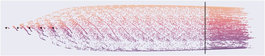
agents With a low spatial agent density, the Figure 6. Spatial Positions on Intersection Environment
subpolicies converge to a roundabout motion. Agents trained in an 8 agent environment cross the intersection
On increasing the spatial density, the agents in two discrete lanes on the right hand side of the road. The
learn to jointly obey the traffic signals and chosen lane depends on the starting positions of the agents.
lanes. Agents trained with higher spatial den- Agents starting towards the left tend to take the inner lane to
sity follow two lanes exclusively on one side allow a faster traffic flow.
of the road.
5.2 E MERGENCE OF L ANES
To analyze lane emergence, we relax the constraint on the fixed agent paths in the setup of Section 5.1.
We use the Bilevel PPO Algorithm (Section 4.4) to train the two subpolicies. The spline subpolicy
predicts a deviation from a path along the roads’ central axis connecting the start position to the
destination, similar to the GPS navigation maps used by human drivers. The acceleration subpolicy
uses the same formulation as Section 5.1.
To empirically analyze the emergence of lanes, we plot the “Normalized Lane Position" of the agents
over time. “Normalized Lane Position" is the directional deviation of agent from the road axis. We
consider the right side of the road (in the ego frame) to have a positive “Normalized Lane Position".
6Published as a conference paper at ICLR 2021
Figures 4 & 5 show the variation with lidar noise and number of training agents respectively. Figure 6
shows the spatial positions of the agents for the 8 agent perfect perception environment.
5.3 R IGHT OF WAY
For tasks that can be performed simultaneously and take approximately equal time for completion,
First In First Out (FIFO) scheduling strategy minimizes the average waiting time. In the context of
driving through an intersection where each new agent symbolizes a new task, the agent that arrives
first at the intersection should also be able to leave the intersection first. In other words, given any
two vehicles, the vehicle arriving at the intersection first has the “right of way" over the other vehicle.
Let the time at which agent i ∈ [n] arrives at the intersection be (ta )i and leaves the intersection be
(td )i . If ∃j ∈ [n] \ {i}, such that (ta )i < (ta )j and (td )i > (td )j , we say that agent i doesn’t respect
j’s right of way. We evaluate this metric on a model trained on a nuScenes intersection (Figure 8).
We observe that, at convergence, the agents follow this right of way 85.25 ± 8.9% of time (Figure 7).
0.14 Speaker Consistency
90 70 |Pearson Coefficient| 0.4
Agents obeying Right of Way (%)
0.12
60
Speaker Consistency
|Pearson Coefficient|
80 0.10
Agents Crashed (%)
0.3
70 50
0.08
60 40 0.2
0.06
50 30
0.04
0.1
40 20
0.02
30 10
0 20 40 60 80 100
0.0 0.2 0.4 0.6 0.8 1.0 1.2 LiDAR Noise (%)
Number of Training Episodes 1e7
Figure 8. nuScenes In-
Figure 7. Right of Way Agents are tersection used for Right Figure 9. Emergent Communica-
increasing able to successfully reach tion with Perception Noise Speaker
of Way (see Section 5.3) Consistency & Pearson coefficient be-
their destinations (denoted by the de- and Communication (see Sec-
creasing red line) with more training tween the agent’s heading and its sent
tion 5.4) Training and Evalu- message increase with increase in Per-
episodes. The agents also increasing ation. The red and green dots
obey the right of way (denoted by the ception Noise. Since all agents have
mark the location of the traf- faulty sensors, the agents aid each other
increasing green line). The error bars fic signals and their current
are constructed using µ ± σ2 . to navigate by propagating their head-
ternary state. ing to their trailing car.
5.4 C OMMUNICATION
One way to safely traverse an intersection is to signal one’s intention to nearby vehicles. We analyze
the impact of perception noise on emergent communication at an intersection (Figure 8). In particular,
we measure the Speaker Consistency (SC), proposed in Jaques et al. (2019). SC can be considered
as the mutual information between an agent’s message and its future action. We report the mutual
information and the Pearson coefficient (Freedman et al., 2007) between the agent’s heading and its
sent message. We limit the communication channel to one bit for simplicity. Each car only receives a
signal from the car in the front within −30◦ and 30◦ . Figure 9 shows that agents rely more heavily
on communication at intersections when perception becomes less reliable.
5.5 FAST L ANES ON A H IGHWAY
Highways have dedicated fast lanes to allow a smooth flow of traffic. In this experiment, we
empirically show that autonomous vehicles exhibit a similar behavior of forming fast lanes while
moving on a highway when trained to maximize traffic flow. We consider a straight road with a
uni-directional flow of traffic. Agents are spawned at random positions along the road’s axis.
0.9
Acceleration Rating
0.8
0.7
0.6
Figure 10. Spatial Positioning in Highway Environment Agents start from one of the positions marked by
?, and need to reach the end position represented by the solid black line. The agents with a higher acceleration
rating move on the right hand side while the lower rated ones drive on the left hand side.
7Published as a conference paper at ICLR 2021
Every agent is assigned a scalar value called “Acceleration Rating," which scales the agent’s accelera-
tion and velocity limits. Thus, a higher acceleration rating implies a faster car. The spline subpolicy
predicts an optimal spline considering this acceleration rating. Even though the agents can decide
to move straight by design, it is clearly not an optimal choice as slower cars in front will hinder
smooth traffic flow. Figure 10 shows that agents are segregated into different lanes based on their
Acceleration Rating. Figure 11 visualizes this behavior over time.
Time Step = 0 Time Step = 5 Time Step = 10 Time Step = 15
Normalized Lane Position
0.5
0.0
0.5
0.5 0.6 0.7 0.8 0.9 1.0 0.5 0.6 0.7 0.8 0.9 1.0 0.5 0.6 0.7 0.8 0.9 1.0 0.5 0.6 0.7 0.8 0.9 1.0
Acceleration Rating Acceleration Rating Acceleration Rating Acceleration Rating
Figure 11. Fast Lane Emergence Visualization of rollouts from a 10-agent highway environment. In y-axis,
we show the agent’s position relative to the axis of the road normalized by road width. The agents reach a
consensus where the faster agents end up on the right-hand side lane. This pattern ensures that slower vehicles
do not obstruct faster vehicles once the traffic flow has reached a steady state.
5.6 M INIMUM D ISTANCE B ETWEEN V EHICLES
25
In this task, we evaluate the extent to which the agents Safe Driving
Speed-Matching Distance (m)
learn to respect a minimum safety distance between 20
agents while driving. When agents are too close, they 15
are at a greater risk of colliding; when agents are too 10
far, they are not as efficient traveling a → b.
5
2amax
∆s2
To derive a human-like “safety distance”, we assume 0
agents can change their velocity according to v 2 =
0 5 10 15 20 25
Distance to Leading Car (m)
u2 + 2ad, where v and u are the final and initial Figure 12. Safety Distance Maintained in
velocities respectively, a is acceleration, and d is the Nuscenes Environment Agents need to maintain
distance for which the acceleration remains constant. a minimum of the Speed-Matching Distance to be
Hence, for an agent to stop entirely from a state with able to safely stop. 98.45% of the agents in this
v02 plot learn to respect this distance threshold.
velocity v0 , it needs at least a distance of 2amax in
front of it, where amax is the maximum possible deceleration of the agent.
Our agents perceive the environment through LiDAR; thus, agents can estimate nearby agents’
velocity and acceleration. We define the safe distance as the distance needed for a trailing agent to
have a zero velocity in the leading agent’s frame. We assume that the leading agent travels with a
2
constant velocity, and as such, the safe distance is defined by 2a∆s
max
, where ∆s is the relative velocity.
Any car having a distance greater than this can safely slow down. Agents trained on nuScenes
Intersections obey this safety distance around 98.45% time (Figure 12).
30
Speed Matching Distance (m)
0.04 Time Step = 5 Safe Driving
Time Step = 7 25
RL Agent
Time Step = 9
0.03 Time Step = 11 20
Time Step = 13
15
0.02
10
0.01
5
2amax
s2
0.00 0
0 10 20 30 40 50 60 0 5 10 15 20 25 30
Distance from Nearest Pedestrian (m) Actual Distance to Nearest Pedestrian (m)
Figure 13. Safety Distance from Pedestrians We observe that most of the agents maintain a distance greater
than the recommended speed-matching distance from the pedestrians. The shaded region in the KDE plots
indicate the 95% confidence interval and the dotted line is the sample mean
5.7 S LOWING DOWN NEAR A C ROSSWALK
In this task, we evaluate if agents can detect pedestrians and slow down in their presence. We augment
the environment setup of Sec. 5.5, to include a crosswalk where at most 10 pedestrians are spawned
at the start of every rollout. The pedestrians cross the road with a constant velocity. If any agent
collides with a pedestrian, they get a collision reward of -1, and the simulation for that agent stops.
8Published as a conference paper at ICLR 2021
The KDE plots in Figure 13 show that the agents indeed detect the pedestrians, and most of them
maintain a distance greater than 6m. To determine if the agents can safely stop and prevent collision
2
with the pedestrians, we calculate a safe stopping distance of 2asmax , where s is the velocity of the
agent. In the scatter plot, we observe that most agents adhere to this minimum distance and drive at a
distance, which lies in the safe driving region.
6 D ISCUSSION
Safety Distance in Human Driving Safety Distance in RL Agent Driving
25 25
Speed-Matching Distance (m)
Safe Driving Safe Driving
20 20
15 15
10 10
5
5
2amax
∆s2
0
0
0 5 10 15 20 25 0 5 10 15 20 25
Distance to Leading Car (m) Distance to Leading Car (m)
Figure 14. Safety Distance for Humans vs. Safety Distance for RL Agents The agents trained in our MDP
(right) tend to violate the safety distance slightly more than human drivers (left) (98.45% vs. 99.56%), but in
both cases a safety distance is observed the vast majority of the time (green triangular region).
6.1 S TATISTICS OF H UMAN D RIVING
In some cases, the same statistics accumulated over agent trajectories that we use in Section 5 to
quantitatively demonstrate emergence can also be accumulated over the human driving trajectories
labeled in the nuScenes dataset. In Figure 14, we visualize safety distance statistics across nuScenes
trajectories and safety distance statistics across RL agents trained on nuScenes intersections side-
by-side. The nuScenes trainval split contains 64386 car instance labels, each with an associated
trajectory. For each location along the trajectory, we calculate the safety distance as described in
Section 5.6. The same computation is performed over RL agent trajectories. The agents trained in our
MDP tend to violate the safety distance more than human drivers. However, in both cases, a safety
distance is observed the vast majority of the time (green triangular region).
6.2 F UTURE W ORK
By parameterizing policies such that agents must follow the curve generated by the spline subpolicy
at initialization (see Section 4.4), we prevent lane change behavior from emerging. The use of a more
expressive action space should address this limitation at the cost of training time. Additionally, the
fact that our reward is primarily based on agents reaching destinations means that convergence is slow
on maps that are orders of magnitude larger than the vehicles’ dimensions. One possible solution to
training agents to navigate large maps would be to generate a curriculum of target destinations, as in
Mirowski et al. (2018).
7 C ONCLUSION
In this paper, we identify a lightweight multi-agent MDP that empirically captures the driving
problem’s essential features. We equip our agents with a sparse LiDAR sensor and reward agents
when they reach their assigned target destination as quickly as possible without colliding with other
agents in the scene. We observe that agents in this setting rely on a shared notion of lanes and traffic
lights to compensate for their noisy perception. We believe that dense multi-agent interaction and
perception noise are critical ingredients in designing simulators that seek to instill human-like road
rules in self-driving agents.
8 ACKNOWLEDGEMENT
This work was supported by NSERC and DARPA’s XAI program. SF acknowledges the Canada
CIFAR AI Chair award at the Vector Institute. AP acknowledges support by the Vector Institute.
9Published as a conference paper at ICLR 2021
R EFERENCES
Joshua Achiam. Spinning Up in Deep Reinforcement Learning. 2018.
Adrian K Agogino and Kagan Tumer. Unifying temporal and structural credit assignment problems.
2004.
Bowen Baker, Ingmar Kanitscheider, Todor Markov, Yi Wu, Glenn Powell, Bob McGrew, and Igor
Mordatch. Emergent tool use from multi-agent autocurricula. arXiv preprint arXiv:1909.07528,
2019.
Mayank Bansal, Alex Krizhevsky, and Abhijit S. Ogale. Chauffeurnet: Learning to drive by imitating
the best and synthesizing the worst. CoRR, abs/1812.03079, 2018. URL http://arxiv.org/
abs/1812.03079.
F. Belletti, Daniel Haziza, Gabriel Gomes, and A. Bayen. Expert level control of ramp metering
based on multi-task deep reinforcement learning. IEEE Transactions on Intelligent Transportation
Systems, 19:1198–1207, 2018.
Alex Bewley, Jessica Rigley, Yuxuan Liu, Jeffrey Hawke, Richard Shen, Vinh-Dieu Lam, and Alex
Kendall. Learning to drive from simulation without real world labels. CoRR, abs/1812.03823,
2018. URL http://arxiv.org/abs/1812.03823.
Raunak P Bhattacharyya, Derek J Phillips, Changliu Liu, Jayesh K Gupta, Katherine Driggs-Campbell,
and Mykel J Kochenderfer. Simulating emergent properties of human driving behavior using
multi-agent reward augmented imitation learning. In 2019 International Conference on Robotics
and Automation (ICRA), pages 789–795. IEEE, 2019.
Mariusz Bojarski, Davide Del Testa, Daniel Dworakowski, Bernhard Firner, Beat Flepp, Prasoon
Goyal, Lawrence D. Jackel, Mathew Monfort, Urs Muller, Jiakai Zhang, Xin Zhang, Jake Zhao,
and Karol Zieba. End to end learning for self-driving cars. CoRR, abs/1604.07316, 2016. URL
http://arxiv.org/abs/1604.07316.
Lucian Busoniu, Robert Babuska, and Bart De Schutter. A comprehensive survey of multiagent
reinforcement learning. IEEE Transactions on Systems, Man, and Cybernetics, Part C (Applications
and Reviews), 38(2):156–172, 2008.
Holger Caesar, Varun Bankiti, Alex H. Lang, Sourabh Vora, Venice Erin Liong, Qiang Xu, Anush
Krishnan, Yu Pan, Giancarlo Baldan, and Oscar Beijbom. nuScenes: A multimodal dataset for
autonomous driving. arXiv preprint arXiv:1903.11027, 2019.
Edwin Catmull and Raphael Rom. A class of local interpolating splines. In Computer aided geometric
design, pages 317–326. Elsevier, 1974.
Boyuan Chen, Shuran Song, Hod Lipson, and Carl Vondrick. Visual hide and seek. In Artificial Life
Conference Proceedings, pages 645–655. MIT Press, 2020.
Alexey Dosovitskiy, Germán Ros, Felipe Codevilla, Antonio M. López, and Vladlen Koltun. CARLA:
an open urban driving simulator. CoRR, abs/1711.03938, 2017. URL http://arxiv.org/
abs/1711.03938.
Jakob Foerster, Ioannis Alexandros Assael, Nando De Freitas, and Shimon Whiteson. Learning to
communicate with deep multi-agent reinforcement learning. In Advances in neural information
processing systems, pages 2137–2145, 2016.
David Freedman, Robert Pisani, and Roger Purves. Statistics (international student edition). Pisani,
R. Purves, 4th edn. WW Norton & Company, New York, 2007.
Pablo Hernandez-Leal, Michael Kaisers, Tim Baarslag, and Enrique Munoz de Cote. A survey of learn-
ing in multiagent environments: Dealing with non-stationarity. arXiv preprint arXiv:1707.09183,
2017.
Pablo Hernandez-Leal, Bilal Kartal, and Matthew E. Taylor. A survey and critique of multiagent
deep reinforcement learning. Autonomous Agents and Multi-Agent Systems, 33:750 – 797, 2019.
10Published as a conference paper at ICLR 2021
Max Jaderberg, Wojciech M Czarnecki, Iain Dunning, Luke Marris, Guy Lever, Antonio Garcia
Castaneda, Charles Beattie, Neil C Rabinowitz, Ari S Morcos, Avraham Ruderman, et al. Human-
level performance in 3d multiplayer games with population-based reinforcement learning. Science,
364(6443):859–865, 2019.
Natasha Jaques, Angeliki Lazaridou, Edward Hughes, Caglar Gulcehre, Pedro Ortega, DJ Strouse,
Joel Z Leibo, and Nando De Freitas. Social influence as intrinsic motivation for multi-agent deep
reinforcement learning. In International Conference on Machine Learning, pages 3040–3049.
PMLR, 2019.
Joel Z. Leibo, Edward Hughes, Marc Lanctot, and Thore Graepel. Autocurricula and the emergence
of innovation from social interaction: A manifesto for multi-agent intelligence research. CoRR,
abs/1903.00742, 2019. URL http://arxiv.org/abs/1903.00742.
Siqi Liu, Guy Lever, Josh Merel, Saran Tunyasuvunakool, Nicolas Heess, and Thore Graepel.
Emergent coordination through competition. arXiv preprint arXiv:1902.07151, 2019.
Ryan Lowe, Yi I Wu, Aviv Tamar, Jean Harb, OpenAI Pieter Abbeel, and Igor Mordatch. Multi-agent
actor-critic for mixed cooperative-competitive environments. In Advances in neural information
processing systems, pages 6379–6390, 2017.
Sivabalan Manivasagam, Shenlong Wang, Kelvin Wong, Wenyuan Zeng, Mikita Sazanovich, Shuhan
Tan, Bin Yang, Wei-Chiu Ma, and Raquel Urtasun. Lidarsim: Realistic lidar simulation by
leveraging the real world, 2020.
Eric Medvet, Alberto Bartoli, and Jacopo Talamini. Road traffic rules synthesis using grammatical
evolution. In European Conference on the Applications of Evolutionary Computation, pages
173–188. Springer, 2017.
Piotr Mirowski, Matthew Koichi Grimes, Mateusz Malinowski, Karl Moritz Hermann, Keith An-
derson, Denis Teplyashin, Karen Simonyan, Koray Kavukcuoglu, Andrew Zisserman, and Raia
Hadsell. Learning to navigate in cities without a map. CoRR, abs/1804.00168, 2018. URL
http://arxiv.org/abs/1804.00168.
Volodymyr Mnih, Koray Kavukcuoglu, David Silver, Alex Graves, Ioannis Antonoglou, Daan
Wierstra, and Martin A. Riedmiller. Playing atari with deep reinforcement learning. CoRR,
abs/1312.5602, 2013. URL http://arxiv.org/abs/1312.5602.
Frans A Oliehoek, Christopher Amato, et al. A concise introduction to decentralized POMDPs,
volume 1. Springer, 2016.
OpenAI. Openai five. https://blog.openai.com/openai-five/, 2018.
P. Peng, Quan Yuan, Ying Wen, Y. Yang, Zhenkun Tang, Haitao Long, and Jun Wang. Multiagent
bidirectionally-coordinated nets for learning to play starcraft combat games. ArXiv, abs/1703.10069,
2017.
Jonah Philion and Sanja Fidler. Lift, splat, shoot: Encoding images from arbitrary camera rigs by
implicitly unprojecting to 3d. In Proceedings of the European Conference on Computer Vision,
2020.
Tabish Rashid, Mikayel Samvelyan, Christian Schroeder De Witt, Gregory Farquhar, Jakob Foerster,
and Shimon Whiteson. Qmix: Monotonic value function factorisation for deep multi-agent
reinforcement learning. arXiv preprint arXiv:1803.11485, 2018.
John Schulman, Philipp Moritz, Sergey Levine, Michael Jordan, and Pieter Abbeel. High-dimensional
continuous control using generalized advantage estimation. arXiv preprint arXiv:1506.02438,
2015.
John Schulman, Filip Wolski, Prafulla Dhariwal, Alec Radford, and Oleg Klimov. Proximal policy
optimization algorithms. arXiv preprint arXiv:1707.06347, 2017.
Alexander Sergeev and Mike Del Balso. Horovod: fast and easy distributed deep learning in
TensorFlow. arXiv preprint arXiv:1802.05799, 2018.
11Published as a conference paper at ICLR 2021
Yoav Shoham, Rob Powers, and Trond Grenager. If multi-agent learning is the answer, what is the
question? Artificial intelligence, 171(7):365–377, 2007.
Kyunghwan Son, Daewoo Kim, Wan Ju Kang, David Earl Hostallero, and Yung Yi. Qtran: Learning
to factorize with transformation for cooperative multi-agent reinforcement learning. arXiv preprint
arXiv:1905.05408, 2019.
Matt Stevens and Christopher Yeh. Reinforcement learning for traffic optimization. Stanford. edu,
2016.
Sainbayar Sukhbaatar, Rob Fergus, et al. Learning multiagent communication with backpropagation.
In Advances in neural information processing systems, pages 2244–2252, 2016.
Richard S Sutton, David A McAllester, Satinder P Singh, and Yishay Mansour. Policy gradient meth-
ods for reinforcement learning with function approximation. In Advances in neural information
processing systems, pages 1057–1063, 2000.
Quinlan Sykora, Mengye Ren, and Raquel Urtasun. Multi-agent routing value iteration network.
arXiv preprint arXiv:2007.05096, 2020.
Jacopo Talamini, Alberto Bartoli, Andrea De Lorenzo, and Eric Medvet. On the impact of the rules
on autonomous drive learning. Applied Sciences, 10(7):2394, 2020.
Tonghan Wang, Heng Dong, Victor Lesser, and Chongjie Zhang. Roma: Multi-agent reinforcement
learning with emergent roles, 2020.
David H Wolpert and Kagan Tumer. Optimal payoff functions for members of collectives. In
Modeling complexity in economic and social systems, pages 355–369. World Scientific, 2002.
Cathy Wu, Aboudy Kreidieh, Eugene Vinitsky, and Alexandre M. Bayen. Emergent behaviors in
mixed-autonomy traffic. volume 78 of Proceedings of Machine Learning Research, pages 398–407.
PMLR, 13–15 Nov 2017a. URL http://proceedings.mlr.press/v78/wu17a.html.
Cathy Wu, Aboudy Kreidieh, Eugene Vinitsky, and Alexandre M Bayen. Emergent behaviors in
mixed-autonomy traffic. In Conference on Robot Learning, pages 398–407, 2017b.
Zhenpei Yang, Yuning Chai, Dragomir Anguelov, Yin Zhou, Pei Sun, Dumitru Erhan, Sean Rafferty,
and Henrik Kretzschmar. Surfelgan: Synthesizing realistic sensor data for autonomous driving,
2020.
W. Zeng, W. Luo, S. Suo, A. Sadat, B. Yang, S. Casas, and R. Urtasun. End-to-end interpretable neural
motion planner. In 2019 IEEE/CVF Conference on Computer Vision and Pattern Recognition
(CVPR), pages 8652–8661, 2019.
Ming Zhou, Jun Luo, Julian Villella, Yaodong Yang, David Rusu, Jiayu Miao, Weinan Zhang,
Montgomery Alban, Iman Fadakar, Zheng Chen, Aurora Chongxi Huang, Ying Wen, Kimia
Hassanzadeh, Daniel Graves, Dong Chen, Zhengbang Zhu, Nhat Nguyen, Mohamed Elsayed,
Kun Shao, Sanjeevan Ahilan, Baokuan Zhang, Jiannan Wu, Zhengang Fu, Kasra Rezaee, Peyman
Yadmellat, Mohsen Rohani, Nicolas Perez Nieves, Yihan Ni, Seyedershad Banijamali, Alexan-
der Cowen Rivers, Zheng Tian, Daniel Palenicek, Haitham bou Ammar, Hongbo Zhang, Wulong
Liu, Jianye Hao, and Jun Wang. Smarts: Scalable multi-agent reinforcement learning training
school for autonomous driving, 2020.
12You can also read