Harbor and Intra-City Drivers of Air Pollution: Findings from a Land Use Regression Model, Durban, South Africa - MDPI
←
→
Page content transcription
If your browser does not render page correctly, please read the page content below
International Journal of
           Environmental Research
           and Public Health

Article
Harbor and Intra-City Drivers of Air Pollution:
Findings from a Land Use Regression Model, Durban,
South Africa
Hasheel Tularam 1, *, Lisa F. Ramsay 1 , Sheena Muttoo 1 , Rajen N. Naidoo 1 , Bert Brunekreef 2 ,
Kees Meliefste 2 and Kees de Hoogh 3,4
 1    Discipline of Occupational and Environmental Health, University of KwaZulu-Natal,
      Durban 4041, South Africa; ramsayl@ukzn.ac.za (L.F.R.); sheena.muttoo@gmail.com (S.M.);
      naidoon@ukzn.ac.za (R.N.N.)
 2    Institute for Risk Assessment Sciences, Utrecht University, 3508TD Utrecht, The Netherlands;
      B.Brunekreef@uu.nl (B.B.); C.Meliefste@uu.nl (K.M.)
 3    Department of Epidemiology and Public Health, Swiss Tropical and Public Health Institute (Swiss TPH),
      Socinstrasse 57, CH-4002 Basel, Switzerland; c.dehoogh@swisstph.ch
 4    Faculty of Science, University of Basel, CH-4003 Basel, Switzerland
 *    Correspondence: Hasheel.Tularam@gmail.co.za

 Received: 17 June 2020; Accepted: 15 July 2020; Published: 27 July 2020

 Abstract: Multiple land use regression models (LUR) were developed for different air pollutants to
 characterize exposure, in the Durban metropolitan area, South Africa. Based on the European Study of
 Cohorts for Air Pollution Effects (ESCAPE) methodology, concentrations of particulate matter (PM10
 and PM2.5 ), sulphur dioxide (SO2 ), and nitrogen dioxide (NO2 ) were measured over a 1-year period,
 at 41 sites, with Ogawa Badges and 21 sites with PM Monitors. Sampling was undertaken in two
 regions of the city of Durban, South Africa, one with high levels of heavy industry as well as a harbor,
 and the other small-scale business activity. Air pollution concentrations showed a clear seasonal trend
 with higher concentrations being measured during winter (25.8, 4.2, 50.4, and 20.9 µg/m3 for NO2 ,
 SO2 , PM10 , and PM2.5 , respectively) as compared to summer (10.5, 2.8, 20.5, and 8.5 µg/m3 for NO2 ,
 SO2 , PM10 , and PM2.5 , respectively). Furthermore, higher levels of NO2 and SO2 were measured in
 south Durban as compared to north Durban as these are industrial related pollutants, while higher
 levels of PM were measured in north Durban as compared to south Durban and can be attributed
 to either traffic or domestic fuel burning. The LUR NO2 models for annual, summer, and winter
 explained 56%, 41%, and 63% of the variance with elevation, traffic, population, and Harbor being
 identified as important predictors. The SO2 models were less robust with lower R2 annual (37%),
 summer (46%), and winter (46%) with industrial and traffic variables being important predictors.
 The R2 for PM10 models ranged from 52% to 80% while for PM2.5 models this range was 61–76% with
 traffic, elevation, population, and urban land use type emerging as predictor variables. While these
 results demonstrate the influence of industrial and traffic emissions on air pollution concentrations,
 our study highlighted the importance of a Harbor variable, which may serve as a proxy for NO2
 concentrations suggesting the presence of not only ship emissions, but also other sources such as
 heavy duty motor vehicles associated with the port activities.

 Keywords: exposure assessment; land use regression; ship emissions; air pollution monitoring

1. Introduction
    Quantifying an individual’s exposure to air borne pollutants remains a key challenge in
epidemiological studies as the level of exposure depends on both the spatial-temporal dynamics of air

Int. J. Environ. Res. Public Health 2020, 17, 5406; doi:10.3390/ijerph17155406    www.mdpi.com/journal/ijerph
Int. J. Environ. Res. Public Health 2020, 17, 5406                                                   2 of 16

pollution concentrations and the individual’s activities. Each individual has their own unique personal
exposure to air pollution during their daily life, occurring both in indoor and outdoor environments,
and therefore the quantifying process is complex [1]. To determine the effect of these exposures on
health, many of these studies have estimated individual air pollution exposure by making use of air
quality monitoring datasets that are representative of the study area and have also made use of more
complex approaches such as spatial interpolation [2–4].
     Proximity-based estimates, interpolation methods (e.g., kriging and inverse distance weighting)
and more complex atmospheric dispersion models are methods that are commonly being used to
undertake spatial exposure assessments. Proximity-based estimates give some indication of health
impact; however, these do not adequately consider meteorology or source characteristics and can
therefore result in exposure misclassification [5]. Kriging, as an example of a spatial interpolation
method, has been found to be increasingly effective when being applied to regional or national scale
and not at a local scale [6,7]. Dispersion models are able to provide a higher level of accuracy at the
local scale however input data demands and specialized expertise limit its application [5,8].
     As a result, further developing exposure models for epidemiological purposes remains imperative
as these models can typically be used to supplement monitoring datasets where direct measurements
are not available as well as assist by reducing expensive and resource intensive monitoring programs.
Furthermore, the contribution of different air pollutant chemicals can be clearly separated in an
exposure assessment to determine their health effects.
     Air pollution exposure models can be used in health risk assessments, for effectively siting ambient
air quality monitoring networks, and for developing air quality related policies and management plans.
Air quality monitoring instrumentation with high precision, accuracy, and temporal resolution is costly
to deploy. While data obtained from monitoring stations are a useful tool for exposure assessments,
these fixed sites of measurements do not show geographical variations in pollutant dispersion, which is
essential for calculating individual impact. Land use regression (LUR) modelling is an alternative to
these approaches, allowing for the calculation of air pollution concentrations at a high spatial resolution
without requiring a detailed air pollution emissions inventory [3]
     LUR combines the monitoring of air pollution at a number of locations with stochastic modelling
using predictor variables obtained through Geographic Information Systems (GIS). Typical examples
of geographic predictor variables include land use type, population, traffic intensity, topography,
and meteorology. Issues regarding the availability of, or access to, complete and reliable predictor
data (i.e., traffic variables, population or housing density, land use, altitude, topography, meteorology,
and location) can hinder LUR studies, but generally these models offer a reliable alternative to more
complex dispersion models that require detailed meteorological data inputs.
     Published LUR models have been developed for sites in Europe, North America, and Japan [9–13].
Since nitrogen dioxide (NO2 ) has previously shown to correlate well with traffic densities in numerous
LUR assessments, this pollutant has been used as a proxy for traffic emissions. Some LUR studies have
even investigated the importance of incorporating meteorological variables for predicting air pollutant
concentrations [14,15].
     An example of multisite LUR model development and its application is the European Study
of Cohorts for Air Pollution Effects (ESCAPE). The ESCAPE study developed LUR models to
estimate exposure at the residential addresses of cohort participants based on uniform monitoring
campaigns and uniform modelling approaches in 36 study areas located all over Europe [16–19].
Furthermore, within the ESCAPE framework, LUR models have been successfully developed to
estimate the spatial variation of annual mean concentrations for various pollutants including PM [19],
elemental composition [18], nitrogen dioxide (NO2 ), and nitrogen oxides (NOx ) [16]. Since these
models were used extensively to assess the association between long-term exposure to air pollution
and specific health outcomes, it was selected for application in this study.
     This study aims to characterize the spatial distribution of nitrogen dioxide (NO2 ), sulphur
dioxide (SO2 ), particulate matter with an aerodynamic diameter of less than 10 µm (PM10 ) and of less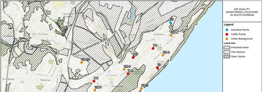
Int. J. Environ. Res. Public Health 2020, 17, 5406 3 of 16
Int. J. Environ. Res. Public Health 2020, 17 3 of 16
than 2.5 µm (PM2.5 ) concentrations in Durban, South Africa, accounting for surrounding land use
variables,
variables, e.g.,
e.g., land
land use
use type
type and
and traffic
traffic intensity. We
We addressed
addressed this
this through
through the
the application
application of
of the
the
ESCAPE
ESCAPE methodology.
Study Background
Study
Durban is
Durban is located
located within
within the
the eThekwini
eThekwini Metropolitan
Metropolitan Municipality
Municipality on on the
the east
east coast
coast of
of South
South
Africa. The
Africa. Themunicipality
municipalityisis home
home toto some
some 3.5
3.5 million
million people
people and
and extends
extends approximately
approximately 50 50 km
km
southwest, 35 km northeast, and 45 km
southwest, km west
west of
of the
the central
central business
business district
district CBD,
CBD, spanning
spanning anan area
area of
of
2
approximately 2297 km (Figure
(Figure 1).
1).
approximately 2
Figure 1. Location of Durban north and Durban south, and their location within South Africa (inset map).
Figure 1. Location of Durban north and Durban south, and their location within South Africa (inset map).
Air pollution in Durban results from a variety of activities. Apart from ship emissions, as it is
Air pollution
the busiest port on intheDurban
Africanresults frompollution
continent, a varietysources
of activities.
includeApart from shiprefining,
petrochemical emissions,pulpas and
it is
the busiest port on the African continent, pollution sources include petrochemical
paper industries, metallurgical industries, organic chemical industries, to smaller facilities such as refining, pulp and
paper industries,
transportation, metallurgical
domestic industries,
fuel burning, organic
landfills, andchemical
quarries industries,
[20]. These to smaller are
industries facilities suchby
regulated as
transportation, domestic fuel burning, landfills, and quarries [20]. These
the South African National Ambient Air Quality Standards, NAAQS (Government Notice 1210 of industries are regulated by
the South
2009) [21]. African National
Air pollution Ambient
sources Air from
ranging Quality Standards,
large industrialNAAQS (Government
facilities, Notice 1210
qualify as regulated of
listed
2009) [21].[22]
activities AirSouth
pollution
Durbansources ranging from
is considered large industrial
the economic facilities, qualifydue
hub of KwaZulu-Natal as regulated listed
to high density
activities [22] South Durban is considered the economic hub of KwaZulu-Natal
of industries within this district. North Durban, however, comprises primarily residential land with due to high density of
aindustries within
limited light this district.
industrial North Durban, however, comprises primarily residential land with a
activity.
limited light industrial activity.
The south Durban and north Durban areas formed the focus of this assessment (Figure 1). The
The South
“Durban south Industrial
Durban and north
Basin” Durban
(DSIB) areas formednarrow
is a well-defined, the focusstripofofthis
land,assessment
approximately(Figure5 km1).
The “Durban
wide, extendingSouth Industrial Basin”from
south-westwards (DSIB)theisDurban
a well-defined,
Harbornarrow strip of land, 12
for approximately approximately
km. It covers 5 km
an
wide, extending south-westwards from the Durban Harbor for approximately
area of approximately 40 km and comprises a mixture of land use zones including industrial,
2 12 km. It covers an area
of approximately
residential, 40 km2 and Historically,
and commercial. comprises a mixture of land
individuals use zones
residing in theincluding
DSIB remainindustrial, residential,
at high risk for
and commercial. Historically, individuals residing in the DSIB remain at high risk
exposure to significant levels of ambient air pollution due to their location to sources of air pollutants. for exposure to
significant levels of ambient air pollution due to their location to sources of
Specifically, two major petroleum refineries, as well as a pulp and paper manufacturing plant areair pollutants. Specifically,
located within the community. The area is linked to other major urban centers via an extensive road
network.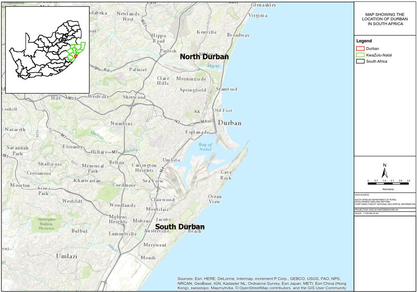
Int. J. Environ. Res. Public Health 2020, 17, 5406                                                4 of 16

two major petroleum refineries, as well as a pulp and paper manufacturing plant are located within
the community. The area is linked to other major urban centers via an extensive road network.
     Since promulgation of the NEM: AQA in 2004, as well as development of the cities Air Quality
Management Plan (AQMP) [23] in 2015, there has been an increased effort towards reducing air
pollution to a level conducive to the health and wellbeing of people living in this area. More stringent
Minimum Emission Standards (MES) [22] being applied in a staged approach over time, have allowed
industries to modify their processes such that they reduce their air pollution impact in the area in
which they operate [24]. The north Durban study area comprises the residential areas of Newlands,
Kenville, Broadway, Virginia as well as light industrial business parks that have developed along the
Umgeni River and along the R102 and Umgeni Road.

2. Materials and Methods
    The ESCAPE methodology was generally applied in this LUR assessment of Durban,
KwaZulu-Natal, South Africa. The methodology employs a mixture of air pollution monitoring
and modelling techniques to estimate exposure at specific GIS locations to ambient air pollution,
accounting for surrounding land use.

2.1. Monitoring Site Selection
     Monitoring sites were selected to best represent the spatial variation of air pollution in north
Durban and South Durban. Regional background, urban sites, and street type-sites were identified
(Figure 2). The urban sites were selected because they were not significantly affected by air pollution
in their direct vicinity, with no more than 3000 vehicles per a day passing within 50 m of the site or
other key air pollution sources (industries, combustion sources, etc.) present within a radius of 100 m.
The street type-site represented traffic pollution and was defined as an area where traffic intensity
exceeded 10,000 vehicles per a day [16]. The regional background sites were located away from local
source activity to represent a long-term average of ambient pollutant concentrations.
     The following criteria were adopted for specific site selection:

•     Monitoring sites were not located within 25 m of a traffic intersection;
•     Monitoring sites were at least 2 m from the roadside;
•     Monitoring sites were not located with 100 m of construction activities; and
•     Sampling points were selected such that airflow around the samplers were unrestricted
      by buildings.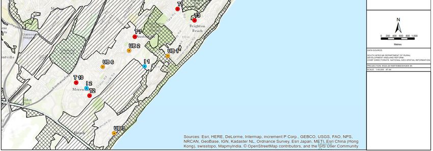
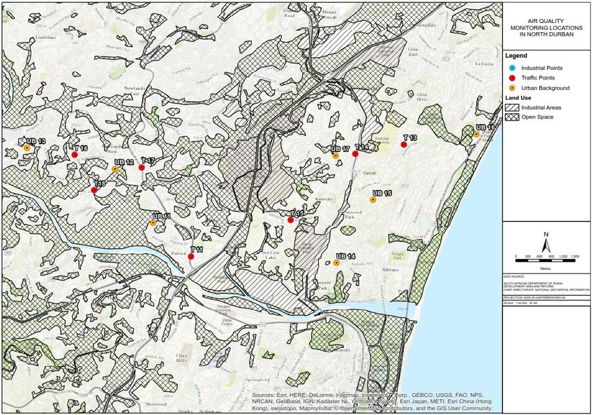
Int. J. Environ. Res. Public Health 2020, 17, 5406 5 of 16
Int. J. Environ. Res. Public Health 2020, 17 5 of 16
Figure 2.
Figure 2. Location of air quality monitoring points in Durban north and
and Durban
Durban south,
south, and
and their
their
location within
location within South
South Africa.
Africa.
2.2. Monitoring Equipment were
Since measurements Installation
not performed continuously, at one additional site (the reference site),
PM, In
NO 2, and
this SO2Ogawa
study, were measured using thewere
passive samplers same instruments
used to measure forNO a period of 1 year (July 2015–June
2 and SO2 concentrations while
2016). This allowed for sites that were only measured
Harvard impactors were used to measure PM10 and PM2.5 concentrations according over the three seasons to be adjusted to the
to standard
long-term average for the monitoring period. As such there were
operating procedures (SOPs) adopted in other ESCAPE studies [25]. PM10 and PM2.5 measurements 21 PM monitoring sites and 41 NO2
and SO
were 2 monitoring
conducted at 20sites in total (Figures
monitoring sites (11 in3 and
south 4).Durban
The reference
and nine siteinwas selected
north Durban) at the University
while passive
NO2 and SO2 measurements were conducted at 40 monitoring sites (23 in south Durban and 17 in of
of KwaZulu-Natal as it is strategically located between north and south Durban where a bulk the
north
monitoring
Durban) was the
within undertaken.
eThekwini Furthermore,
Municipality this
(aslocation
shown was easily 2–4
in Figures accessible
below). asMeasurements
this station required
were
to be fully operational throughout a 1-year period. For quality control
conducted over 2-week periods per a site with a 1-week break in between in the winter (June–August), purposes, one field blank per
a pollutant (PM, NO , and SO ) was collected at
spring (September–November 2015), and summer (December–February) seasons.
2 2 the reference site such that 12 field blanks were
collected
Sinceover the samplewere
measurements period.notThe field blanks
performed were usedattoone
continuously, calculate the limit
additional of detection
site (the referenceofsite),
the
samples. Furthermore, one field duplicate (PM , NO , and SO ) was
PM, NO2 , and SO2 were measured using the same instruments for a period of 1 year (July 2015–June
10 2 2 collected at the reference site for
the measurement period. Field duplicates were logged to determine
2016). This allowed for sites that were only measured over the three seasons to be adjusted to the the accuracy of measured
pollutant concentrations.
long-term Furthermore,
average for the monitoring a rotameter
period. As such was used
there to measure
were the volumetric
21 PM monitoring flow41rate
sites and NOof 2
each Harvard impactor at the start and end of each 2-week monitoring
and SO2 monitoring sites in total (Figures 3 and 4). The reference site was selected at the University period. Further quality
assurance
of details are
KwaZulu-Natal as provided in the Supplementary
it is strategically located between Materials.
north and south Durban where a bulk of the
The particle mass on each filter was
monitoring was undertaken. Furthermore, this location was determined by weighing the filterasbefore
easily accessible and after
this station field
required
sampling. The pump units consist of a 10 liters per a minute pump,
to be fully operational throughout a 1-year period. For quality control purposes, one field blank pertwo timers (a weekly and 24 h),
aand an elapsed
pollutant (PM,time
NOindicator. The total volume of air sampled was recorded using a built-in timing
2 , and SO2 ) was collected at the reference site such that 12 field blanks were
device. The pump unit
collected over the sample period.is built intoTheweatherproof
field blanks case werecomprising of ventilators
used to calculate the limittoofallow the unit
detection of theto
cool should the temperature in the box get too high. The impactors were
samples. Furthermore, one field duplicate (PM10 , NO2 , and SO2 ) was collected at the reference site deployed such that the inlets
were
for theatmeasurement
a height of about period.1.5 mFieldabove the ground.
duplicates were logged to determine the accuracy of measured
Timers were used to allow the
pollutant concentrations. Furthermore, a rotameter pump to operate wasfor 15 to
used min duringthe
measure every 2 h. Allflow
volumetric samples
rate
collected
of were stored
each Harvard impactorat 4 °C.
at thePost 24-h
start andconditioning,
end of eachall filtersmonitoring
2-week were pre and post weighed
period. as per
Further quality
RUPIOH SOP
assurance version
details 3 weighing
are provided in the protocol. SamplesMaterials.
Supplementary were then shipped to University of Utrecht to
test for reflectance and determine the absorption coefficient using a Smoke Stain Reflectometer:
Diffusion Systems Ltd. Model 43 (M43D).Int. J. Environ. Res. Public Health 2020, 17, 5406 6 of 16
Int.
Int. J.J. Environ.
Environ. Res.
Res. Public
Public Health
Health 2020,
2020, 17
17 66 of
of 16
16
Figure 3.
3. Location
Figure 3.
Figure Location of
Location of air
of air quality
air quality monitoring
quality monitoring samplers
monitoring in
samplers in
samplers south
in south Durban.
south Durban.
Durban.
Figure 4.
4. Location
Figure 4.
Figure Location of
Location of air
of air quality
air quality monitoring
quality monitoring samplers
monitoring in
samplers in
samplers north
in north Durban.
north Durban.
Durban.
All
All Ogawa
Ogawa passive
passive samplers
samplers (for
(for NO
NO22 and
and SO
SO22)) were
were deployed
deployed at
at 22 m
m above
above the
the ground
ground at
at each
each
sample
sample point.
point. Upon
Upon collection,
collection, samples
samples were
were stored
stored atat 44 °C
°C before
before being
being couriered
couriered to
to aa South
South African
African
National
National Accredited
Accredited System
System (SANAS)
(SANAS) laboratory
laboratory for
for analysis.
analysis.Int. J. Environ. Res. Public Health 2020, 17, 5406 7 of 16
The particle mass on each filter was determined by weighing the filter before and after field
sampling. The pump units consist of a 10 L per a minute pump, two timers (a weekly and 24 h), and an
elapsed time indicator. The total volume of air sampled was recorded using a built-in timing device.
The pump unit is built into weatherproof case comprising of ventilators to allow the unit to cool should
the temperature in the box get too high. The impactors were deployed such that the inlets were at a
height of about 1.5 m above the ground.
Timers were used to allow the pump to operate for 15 min during every 2 h. All samples collected
were stored at 4 ◦ C. Post 24-h conditioning, all filters were pre and post weighed as per RUPIOH SOP
version 3 weighing protocol. Samples were then shipped to University of Utrecht to test for reflectance
and determine the absorption coefficient using a Smoke Stain Reflectometer: Diffusion Systems Ltd.
Model 43 (M43D).
All Ogawa passive samplers (for NO2 and SO2 ) were deployed at 2 m above the ground at each
sample point. Upon collection, samples were stored at 4 ◦ C before being couriered to a South African
National Accredited System (SANAS) laboratory for analysis.
To determine the annual average for each monitoring site, the results from each 2-week sampling
period had to be adjusted using data from the reference site as monitoring was continuously undertaken
at this point for a period of 1 year. The arithmetic means of the available measurements (i.e., both
sampling periods) per site were adjusted using the difference between the sampling period and the
annual average at the reference site thus deriving an annual adjusted average for each pollutant.
2.3. Geographic Predictor Variables
Important predictor variables as indicated by [9], included traffic, housing density, population
density, land use type, physical geography, and meteorology. The eThekwini Municipality Corporate
GIS Unit provided the geographical information for the study area. GIS shape files collected include
roads, land use, population density, as well as physical geography such as altitude and distance to
coastline. The land use data was divided into industrial, open space, urban, and Harbor.
Road linkages were categorized into two groups (major and minor) based on traffic intensity.
The eThekwini Municipality Traffic Authority provided traffic count data for light duty motor vehicles
(LDMV), and heavy-duty motor vehicles (HDMV) for major intersections along roads in south Durban
and north Durban (period 2013–2017). While road length and distance to road classifications were
also used to determine the effect of traffic on air pollution [3,9], traffic count data was also obtained.
This served to further explore the effect of the number of HDMV and LDMV on the measured air
pollutant concentrations in north Durban and south Durban.
Since wind speed and direction is regarded as a key meteorological parameter in the dispersion of
air pollution, this study also investigated this phenomenon by assessing a wind trajectory in relation
to industry location. Meteorological data in south Durban and north Durban was obtained from the
South African Weather Services meteorological station located at the old Durban International Airport
and Mount Edgecombe, respectively. Hourly wind speed, wind direction, ambient temperature,
and humidity data were processed into annual and seasonal averages. The distance to three main
industries (two multinational refineries and one multinational pulp and paper manufacturer) was
measured and the percentage time the wind blows from the direction of those industries to a receptor.
The selection of buffer radii was based on previous ESCAPE studies [25]. Buffers of 50, 100, 300,
500, and 1000 m for major and minor road length and 1000 m for distance to major and minor roads to
account for background emissions of NO2 , related to traffic emissions were defined. Buffer distances of
100, 300, 500, 1000, and 2000 m were defined for all other variables. Each buffer was used to intersect
the different predictor variables to allow for points, lengths, and areas to be calculated. The predictors
used for the LUR models, buffer size, rational for inclusion, as well as expected direction of effect are
presented in the supplementary material Table S1.Int. J. Environ. Res. Public Health 2020, 17, 5406 8 of 16
2.4. Land Use Regression Modelling
Using the ESCAPE [19,25] approach, standard linear regression was used to develop land use
regression models to predict air pollutant concentrations. The model that yields the highest percentage
explained variability (R2 ) and minimizes the error (root mean square, RMSE) was selected for use.
To develop a regression model for each pollutant, a forward stepwise procedure was followed.
Model validation was undertaken using the leave-one-out cross validation (LOOCV) method.
The model was developed for n − 1 sites and the predicted concentrations compared to the measured
concentration at the left-out site. This process was undertaken N times and the relationship between the
predicted and observed concentrations, across all sites, then computed as a measure of model performance.
All modelling was performed using the Statistical Package STATA version 15 (StataCorp LLC.,
College Station, TX, USA). 53 variables were regressed individually against the NO2, SO2 , PM10 , and
PM2.5 concentrations for each season as well as an annual average for this assessment. As such, a total
12 LUR models were developed.
3. Results
3.1. Air Pollutant Measurements
Overall, 90 SO2 , 100 NO2 , 51 PM10 and PM2.5 measurements were taken over the duration of
the 1-year monitoring period. Intermittent air pollution measurements at the monitoring points were
adjusted in line with monitoring data from the reference site to provide annual averages. A high
correlation was observed for the duplicate NO2 (R2 = 0.92), SO2 (R2 = 0.85), and PM10 (R2 = 0.99)
samplers over the 1-year monitoring period at the reference site. No duplicate samples were collected
for PM2.5 . Adjusted average annual as well as seasonal NO2 , SO2 , PM10 , and PM2.5 concentrations
measured across both north Durban and south Durban are presented in Table 1 below. The N refers to
the number of monitoring points. There were initially 20 PM and 40 NO2 /SO2 monitoring sites, however
points at which outlier measurements were recorded at/or samplers were stolen were completely
removed from the dataset.
Table 1. Adjusted annual average annual and seasonal nitrogen dioxide (NO2 ), sulphur dioxide (SO2 ),
PM10 , and PM2.5 concentrations (µg/m3 ).
Pollutant Season Mean Standard Deviation Minimum Maximum
Annual average 17.0 3.9 6.5 24.0
Summer average 10.5 2.8 4.1 17.3
NO2
Winter average 25.8 6.7 10.1 42.3
Spring Average 20.4 5.1 7.6 29.5
Annual average 3.4 1.6 1.5 7.8
Summer average 2.8 1.3 0.7 6.4
SO2
Winter average 4.2 1.9 1.8 9.2
Spring average 3.3 1.5 1.4 7.4
Annual average 36.6 19.2 11.0 99.7
Summer average 20.5 10.0 9.3 54.1
PM10
Winter average 50.3 27.0 15.2 138.1
Spring average 38.5 21.9 8.91 107.7
Annual average 12.3 5.7 3.2 31.0
Summer average 8.5 4.0 2.2 21.5
PM2.5
Winter average 17.0 8.0 4.5 43.1
Spring average 11.4 5.3 3.1 29.4Int. J. Environ. Res. Public Health 2020, 17, 5406 9 of 16
Box plots of the annual and seasonal concentrations measured in north Durban and south Durban
for each pollutant are presented in supplementary material (Figure S1).
3.2. Land Use Regression Models
In the NO2 models (Table 2), traffic and industrial variables emerged as predictors in expected
directions, as expected across the seasons and in the annual model. Of particular interest was the
role of the Harbor variable, which was a significant predictor in the summer and annual models.
This variable was not a predictor in the modelling of the other pollutants.
Table 2. Annual, summer, and winter NO2 land use regression (LUR) model results.
Standard
Season Predictors Unit R2 LOOCV df Beta t p
Error
Intercept - 1.85 × 101 2.16 × 100 24.5 0.0
Total length major roads
m 2.07 × 10⁻² 1.12 × 10⁻¹ 4.4 0.0
Annual (100 m) 0.6 0.4 32
Harbor (2000 m) m 4.32 × 10⁻⁷ 4.50 × 10⁻³ 1.9 0.0
Elevation m −3.68 × 10⁻² 2.24 × 10⁻⁷ −3.6 0.0
Intercept - 8.32 × 100 6.43 × 10⁻¹ 12.9 0.0
Distance to minor roads m 5.66 × 10⁻² 1.71 × 10⁻² 3.3 0.0
Summer 0.4 0.2 32
Industrial (1000 m) m 1.98 × 10⁻⁶ 8.79 × 10⁻⁷ 2.3 0.0
Harbor (2000 m) m 4.97 × 10⁻⁷ 2.30 × 10⁻⁷ 2.2 0.0
Intercept - 2.44 × 101 1.43 × 100 17.1 0.0
Elevation m −5.25 × 10⁻² 1.58 × 10⁻² −3.3 0.0
Winter 0.6 0.5 30
Population (1000 m) m 8.25 × 10⁻⁴ 1.91 × 10⁻⁴ 4.3 0.0
Industrial (100 m) m 3.75 × 10⁻⁴ 1.61 × 10⁻⁴ 2.3 0.0
Traffic and industrial variables were, as expected, important predictors across the majority of
pollutants. Specific traffic variables varied across the pollutants, with road length serving as a proxy
for the PM10 and the summer PM2.5 models, while the LDMV variable emerged as significant for the
SO2 and PM2.5 models. Indicative of the geography of Durban, elevation was a negative predictor
in the NO2 and PM10 models. However, elevation was not a predictor in the other models (see also
Tables 3–5).
Table 3. Annual, summer, and winter SO2 LUR model results.
Standard
Season Predictors Unit R2 LOOCV df Beta t p
Error
Intercept - 2.5 × 100 3.0 × 10⁻¹ 8.4 0.0
Industrial (500 m) m 7.9 × 10⁻⁶ 1.9 × 10⁻⁶ 4.1 0.0
Annual 0.4 0.2 37
Total number LDMV
No 8.4 × 10⁻⁸ 3.1 × 10⁻⁸ 2.8 0.0
(100 m)
Intercept - 1.4 × 100 3.1 × 10⁻¹ 4.5 0.0
Industrial (2000 m) m 4.1 × 10⁻⁷ 9.9 × 10⁻⁸ 4.1 0.0
Summer 0.5 0.3 29
Total number LDMV
No 7.1 × 10⁻⁸ 2.2 × 10⁻⁸ 3.2 0.0
(100 m)
Intercept - 2.6 × 100 5.7 × 10⁻¹ 4.6 0.0
Industrial (2000 m) m 5.9 × 10⁻⁷ 1.9 × 10⁻⁷ 3.1 0.0
Winter 0.5 0.4 29
Total number LDMV
No 3.5 × 10⁻⁸ 1.7 × 10⁻⁸ 2.1 0.0
(300 m)Int. J. Environ. Res. Public Health 2020, 17, 5406 10 of 16
Table 4. Annual, summer, and winter PM10 LUR model results.
Standard
Season Predictors Unit R2 LOOCV df Beta t p
Error
Intercept - 3.2 × 101 2.2 × 100 14.0 0.0
Total length major road
Annual m 0.8 0.7 14 5.3 × 10⁻³ 8.8 × 10⁻⁴ 6.0 0.0
(1000 m)
Elevation m −1.1 × 10⁻¹ 4.4 × 10⁻² −2.4 0.0
Intercept - 1.2 × 101 2.4 × 100 5.1 0.0
Population (2000 m) m 2.3 × 10⁻⁴ 7.1 × 10⁻⁵ 3.3 0.0
Summer 0.5 0.2 13
Total number HDMV
No 8.8 × 10⁻⁶ 4.2 × 10⁻⁶ 2.1 0.0
(100 m)
Intercept - 2.5 × 101 9.7 × 100 2.6 0.0
Total length major road
m 4.4 × 10⁻³ 1.8 × 10⁻³ 2.5 0.0
Winter (1000 m) 0.8 0.6 13
Elevation m −1.9 × 10⁻¹ 6.5 × 10⁻² −3.0 0.0
Urban (2000 m) m 4.0 × 10⁻⁶ 2.0 × 10⁻⁶ 2.0 0.0
Table 5. Annual, summer, and winter PM2.5 LUR model results.
Standard
Season Predictors Unit R2 LOOCV df Beta t p
Error
Intercept - 1.1 × 101 7.9 × 10⁻¹ 14.0 0.0
Open space (100 m) m −2.2 × 10⁻⁴ 7.2 × 10⁻⁵ −3.1 0.0
Annual Total number LDMV 0.8 0.6 13
No 1.8 × 10⁻⁷ 5.6 × 10⁻⁸ 3.2 0.0
(100 m)
Population (2000 m) m 5.3 × 10⁻⁵ 2.3 × 10⁻⁵ 2.4 0.0
Intercept - 7.6 × 100 5.9 × 10⁻¹ 13.0 0.0
Summer Total length major road 0.7 0.7 15
m 2.4 × 10⁻³ 4.0 × 10⁻⁴ 6.0 0.0
(500 m)
Intercept - −8.9 × 100 4.8 × 100 −0.19 0.0
Total number LDMV
Winter No 0.6 0.6 14 2.5 × 10⁻⁷ 1.3 × 10⁻⁷ 2.0 0.0
(100 m)
Urban (100 m) m 5.7 × 10⁻⁴ 1.8 × 10⁻⁴ 3.2 0.0
Population emerged as a predictor in only the winter NO2 , summer PM10 , and annual PM2.5
models. Other urban predictors, such as urban space, were significant in the winter models of PM10
and PM2.5 .
In all the pollutant models (annual, summer, and winter) VIF was considered reasonable (Int. J. Environ. Res. Public Health 2020, 17, 5406 11 of 16
LUR models suggesting that the Harbor and its associated activity may be an influential source of
pollution. Durban is the busiest port in Africa and has the second largest container terminal in the
southern hemisphere. For the ease of transporting goods and other commodities to and from the
Harbor, major industries in the region developed around the port. To transport goods for import
and/or export purposes, the South African National Roads Agency Limited Ltd (SANRAL, Pretoria,
South Africa) developed an advanced road network to service the inland cities of the country. As a
result, air pollution is not only emitted from industries in the DSB, but also from vehicles that transport
goods to and from the port [26].
A recent study demonstrated that the total annual NO2 emissions from ships in the Durban Port
were calculated at 1116.87 tonnes per annum and were slightly lower than two petrochemical refineries
emissions of 1760 and 1241 tonnes per annum in 2010 and 2011, respectively [27]. These results
show that the port emissions should not be ignored in cumulative air quality impact assessments.
Furthermore, the study shows a higher number of vessels frequenting the terminal between May and
September, suggesting reason for the Harbor variable being present in the winter NO2 LUR model.
A study making use of the operational meteorological air quality model (OML) to calculate
the urban dispersion of air pollutants originating from ships in three Danish ports, Copenhagen,
Elsinore, and Koge, showed that oxides of nitrogen (NOx ) emitted by ships in the port of Copenhagen
and Elsinore contributed substantially to the overall NOx pollution in their respective areas [28].
Furthermore, in LUR models estimating air pollution exposure of NO2 and NOx in 36 study areas
in Europe, the Harbor variable was statistically significant in models for other port cities such as
Copenhagen, (Denmark), Ruhr Area, (Germany), and Heraklion (Crete) [16].
The monitoring results confirmed a general increase in NO2 , PM10 , PM2.5 , and SO2 concentrations
during winter and a decrease in NO2 , PM10 , PM2.5 , and SO2 concentrations during summer. The results
measured during spring are similar to the annual average and are lower than those measured during
winter and higher than those measured during summer. The nature and characteristics of air pollution
dispersion over Durban is known to fluctuate during the year with the change of the seasons [29].
During winter, the slow moving South Indian High is responsible for clear skies, low levels of
precipitation, and weak north-easterly winds. The frequency and strength of inversions are known to
be greatest during winter months of June and July. Surface inversions trap air pollution by inhibiting
adequate air pollution dispersion.
In a greater volume of atmosphere, the ability for air pollutants to disperse increases and there is
a greater chance for its concentration to be reduced. During summer, mainly unstable conditions are
found to develop, and the depth of the mixing layer is increased thereby enabling free convection of
air into the upper boundary layer. This phenomenon assists air pollutants to disperse into the upper
atmosphere. Conversely, during winter, particularly in the early mornings, stable conditions arise, and
the vertical diffusion of air pollutants is limited. A surface inversion may exist nearer to the ground,
or pollutants may be diffused upward only to be halted by an elevated inversion layer. Both of these
surface and elevated inversions need to be considered in the DSB when analyzing their relationship
with air pollution dispersion.
From a spatial distribution perspective, measured SO2 and NO2 concentrations (annual and
seasonal averages) were higher at the south Durban sites than at the north Durban sites. Key industries
in the DSIB include two major oil refineries, owned by multinational corporations, a multinational
paper and pulp plant, a sugar mill, several chemical industries, the port and some 600 other smaller
industries. Measured PM10 and PM2.5 concentrations (annual and seasonal) were on average higher
at the north Durban sites than the south Durban sites. Besides industrial or vehicular emitters other
possible sources for the high PM concentrations identified in the north are large open fields, regular field
fires, sugar cane fires, and domestic burning of garden and other refuse, plus major earthworks and
construction [30].
In our study, the concentrations of ambient PM10 and PM2.5 , NO2 , and SO2 throughout the mixed
industrial and residential land use types in eThekwini and the subsequent LUR modelling presentInt. J. Environ. Res. Public Health 2020, 17, 5406 12 of 16
interesting variation across the intra-city regions for the different pollutants. Although the study
included a heavy industrialized area, the industry variable did not emerge strongly across all pollutant
LUR models. Traffic variables were consistently statistically significant in all LUR models, and this may
imply that this type of modelling works well for air pollution sources that are localized in extent [31].
Total length major road, distance to minor roads, total number of motor vehicles, urban land use
type, and population, returned positive correlations with PM10 , PM2.5 , and NO2 concentrations while
open space and elevation returned negative correlations. In all (annual and seasonal) models, PM10 ,
PM2.5 , and NO2 levels were influenced by traffic variables as well as population and has this been
demonstrated with other studies [13,32].
Population density (an indication of domestic fuel burning) was present in the winter NO2 ,
summer PM10 , as well as annual PM2.5 LUR models. This is consistent with the findings reported in
other studies [4,16,33], in which the population density variable has been related to these sources of PM.
While it was expected for a traffic variable to have appeared in the winter NO2 model, the population
variable appeared instead, indicating that areas with higher population density are related to higher
NO2 levels during winter.
The open space and elevation variables were seen as having a negative influence in the NO2 ,
PM10 , and PM2.5 concentrations. An increase in open space (areas such as urban forests and parks) can
reduce local NO2 , PM10 , and PM2.5 concentrations and improve respiratory health in the area and has
empirically been shown in other studies [34–36].
The importance of considering elevation as an influential factor for coastal cities has been
highlighted by [37,38]. Elevation exhibited a negative interaction with annual average NO2 and PM10
as well as winter NO2 and PM10 concentrations indicating that elevated areas (i.e., outside of south
Durban) had the lowest NO2 and PM10 levels.
The SO2 LUR models were similar to the NO2 LUR models in that the industrial land use coverage
variable as well as the number of LDMV variables were retained in all annual and season models.
In a study undertaken by [39], the highest SO2 values were also associated with industrial and traffic
emission sources. Industrial emissions associated with stacks that are released at a height, impact the
ground level at a distance away from the source. For very fine scale concentrations in and around the
industrial area, dispersion models may be useful to supplement this model; however, these models
require emission data. The poor strength of the LUR models developed for SO2 , however, suggests
that the industrial land use variables need to be carefully considered when being applied in a LUR
assessment. However, our results agree with the other SO2 LUR studies that R2 values for SO2 tend to
be suppressed [40].
There were no input variables of Harbor in the SO2 LUR model. A recent study which calculated
the pollution from ships in the Durban Port found that SO2 emissions from ships that frequent the port
are far less than that emitted from just two large petrochemical refineries and a paper mill operating
nearby [27]. Therefore, while SO2 is emitted during ship hoteling at the port, the SO2 emissions
from industries located near the port far outweigh the SO2 emissions being released from the ships
hoteling at the Harbor. Furthermore, in a study making use of an operational meteorological air quality
model (OML) to calculate the urban dispersion of air pollutants originating from ships in three Danish
ports, Copenhagen, Elsinore, and Koge, ships in Copenhagen and Elsinore (both Harbors) contribute
insignificantly to urban pollution with respect to SO2 [28]. In Koge, however, the low activity in the
Harbor meant that ships did not significantly affect urban air quality.
In the annual and winter PM10 models as well as summer PM2.5 models, total length major roads
was seen as a significant predictor variable. This likely reflects the major impact of motorized road
traffic emissions as well as road dust being suspended from tire and break wear and tear on PM
levels [19]. Furthermore, In South Africa, a substantial fraction of private cars and most middle and
heavy-duty vehicles make use of diesel as fuel for economic reasons. Other sources of PM such as
large open fields, regular field fires, etc., were not taken into account in the LUR model due to limited
data due a limited number of PM sampling equipment used in this study.Int. J. Environ. Res. Public Health 2020, 17, 5406 13 of 16
While a study undertaken by [41] confirms that sea spray does contribute to PM levels at coastal
cities, distance to coastline was not regarded as insignificant predictor variable in the results. The Bluff
Ridge between the ocean and DSIB which acts as a buffer to sea spray to samplers located in the south
Durban could be attributed to PM having a poor relationship with distance to coastline. In north
Durban, samplers were located from approximately 2 km inland of the ocean. Sea spray is known to
decrease with increasing distance away from the shoreline [42].
To determine the effects of change in wind regime during each season, the inclusion of wind
direction as a meteorological variable, which assessed the percentage time wind blows from the two
refineries and the paper mill towards each monitoring point, was assessed. The inclusion of wind
direction in relation to direction of industry however was not regarded as a significant predictor
variable in this study. Furthermore, the inclusion of annual and seasonal average wind speed, ambient
temperature, and humidity also did not emerge as significant variables.
A similar LUR study was undertaken to explain the spatial variation of ambient NOx concentrations
in Durban south [43]. In this study, two 2-week NOx monitoring campaigns were undertaken during
summer and winter and an adjusted annual average was used for the model development. Our study
serves to build onto the work already undertaken by Muttoo et al. (2016) [43] by developing annual
and seasonal LUR models for additional air pollutants (e.g., NO2 , SO2 , PM10 , and PM2.5 ) across
Durban north and Durban south areas. This was achieved by undertaking a more comprehensive
air pollution monitoring campaign for three periods of 2 weeks per a site in the cold, warm, and one
intermediate temperature season between July 2015 and March 2016 as well as taking measurements at
one additional site (reference site) for 1 year. Furthermore, our study was the first to explore the effect
of meteorology on measured pollutant concentrations, in South Africa, given the unique topographical
domain of our study area. The key similarity in the findings of the annual NOx model developed by
Muttoo et al. (2016) [43] and our annual NO2 model was the presence of the traffic variable, suggesting
a strong influence of traffic on NOx related components.
5. Conclusions
In conclusion, while findings of the study highlighted the importance of traffic and land use
type (more specifically, industry) variables in influencing air pollutant concentrations, interestingly
the Harbor variable also emerged as a significant predictor. It is acknowledged that a key limitation
of the study is the sample size used to develop the LUR models especially for PM due to restricted
resources available. Furthermore, the inability of the model to consistently identify industrial land
use also suggests a modelling limitation. The LUR model may not be the ideal tool when estimating
industrial emissions from stacks as the resultant plume would only reach ground level some distance
away from the source. A further improvement of the LUR models could include predictor variables
that characterize industrial emissions in order to capture local variations due to emission patterns [44].
An air pollution dispersion model, which incorporates meteorological data at a high resolution
(example hourly), terrain, physical, and chemical characteristics of the air pollution is recommended to
simulate the formation and transport of the plume, suggesting the need for hybrid modelling [45].
Supplementary Materials: The following are available online at http://www.mdpi.com/1660-4601/17/15/5406/s1,
Figure S1: Distribution of NO2 , SO2 , PM10 , PM2.5 annual and seasonal means for Durban north and Durban
south. Median, interquartile range (IQR), and whiskers present, Table S1: Variables used, buffer radius, rational
for inclusion, and expected direction of effect.
Author Contributions: Conceptualization, L.F.R. and S.M.; Methodology, K.M.; Resources, B.B.; Supervision,
R.N.N. and K.d.H.; Writing—original draft, H.T. All authors have read and agree to the published version of
the manuscript.
Funding: This research received no external funding.
Acknowledgments: We would like to thank the MACE Project Manager Kareshma Asharam and all field
workers (Nigel Govender, Thirushan Nadar, and Teague Landsberg), who assisted with the monitoring campaign.
The eThekwini Municipality Health Unit and Corporate GIS department for the provision of ambient air quality
monitoring station and GIS data, respectively. Sanjeev Sewnarain from South African Weather Services (SAWS)Int. J. Environ. Res. Public Health 2020, 17, 5406 14 of 16
for the provision of meteorological data. We are also grateful for the financial assistance received from the South
African National Research Foundation (NRF) (90550), as well as the South African Medical Research Council
(SAMRC), Astrazenca and the University of KwaZulu-Natal. We extend our appreciation to Institute of Risk
Assessment Sciences (IRAS) for their collaboration in this study.
Conflicts of Interest: The authors declare no conflict of interest.
References
1. Dias, D.; Tchepel, O. Spatial and Temporal Dynamics in Air Pollution Exposure Assessment. Int. J. Environ.
Res. Public Health 2018, 15, 558. [CrossRef] [PubMed]
2. Achakulwisut, P.; Brauer, M.; Hystad, P.; Anenberg, S.C. Global, national, and urban burdens of paediatric
asthma incidence attributable to ambient NO2 pollution: Estimates from global datasets. Lancet Planet. Health
2019, 3, e166–e178. [CrossRef]
3. Bauer, M.; Hoek, G.; Van Vliet, P.; Meliefste, K.; Fischer, P.; Gehring, U.; Heinrich, J.; Cyrys, J.; Bellander, T.;
Lewné, M.; et al. Estimating Long-Term Average Particulate Air Pollution Concentrations: Application of
Traffic Indicators and Geographic Information Systems. Epidemiology 2003, 14, 228–239. [CrossRef] [PubMed]
4. Saucy, A.; Röösli, M.; Künzli, N.; Tsai, M.-Y.; Sieber, C.; Olaniyan, T.; Baatjies, R.; Jeebhay, M.F.; Davey, M.;
Flückiger, B.; et al. Land Use Regression Modelling of Outdoor NO2 and PM2.5 Concentrations in Three Low
Income Areas in the Western Cape Province, South Africa. Int. J. Environ. Res. Public Health 2018, 15, 1452.
[CrossRef] [PubMed]
5. Jerrett, M.; Arain, A.; Kanaroglou, P.; Beckerman, B.; Potoglou, D.; Sahsuvaroglu, T.; Morrison, J.;
Giovis, C.; Arain, M.A. A review and evaluation of intraurban air pollution exposure models. J. Expo. Sci.
Environ. Epidemiol. 2005, 15, 185–204. [CrossRef]
6. Bell, M. The use of ambient air quality modeling to estimate individual and population exposure for human
health research: A case study of ozone in the Northern Georgia Region of the United States. Environ. Int.
2006, 32, 586–593. [CrossRef]
7. Liao, D.; Peuquet, N.J.; Duan, Y.; Whitsel, E.A.; Dou, J.; Smith, R.L.; Lin, H.-M.; Chen, J.-C.; Heiss, G. GIS
Approaches for the Estimation of Residential-Level Ambient PM Concentrations. Environ. Health Perspect.
2006, 114, 1374–1380. [CrossRef]
8. Michanowicz, D.R.; Shmool, J.L.; Tunno, B.J.; Tripathy, S.; Gillooly, S.; Kinnee, E.; Clougherty, J. A hybrid
land use regression/AERMOD model for predicting intra-urban variation in PM2. Atmos. Environ. 2016, 131,
307–315. [CrossRef]
9. Hoek, G.; Beelen, R.; de Hoogh, K.; Vienneau, D.; Gulliver, J.; Fischer, P.; Briggs, D. A review of land-use
regression models to assess spatial variation of outdoor air pollution. Atmos Environ. 2008, 42, 7561–7578.
[CrossRef]
10. Kashima, S.; Yorifuji, T.; Tsuda, T.; Doi, H. Application of land use regression to regulatory air quality data in
Japan. Sci. Total. Environ. 2009, 407, 3055–3062. [CrossRef] [PubMed]
11. Mukerjee, S.; Smith, L.A.; Johnson, M.M.; Neas, L.M.; Stallings, C.A. Spatial analysis and land use regression
of VOCs and NO2 from school-based urban air monitoring in Detroit/Dearborn, USA. Sci. Total. Environ.
2009, 407, 4642–4651. [CrossRef] [PubMed]
12. Ross, Z.; Jerrett, M.; Ito, K.; Tempalski, B.; Thurston, G. A land use regression for predicting fine particulate
matter concentrations in the New York City region. Atmos. Environ. 2007, 41, 2255–2269. [CrossRef]
13. Wheeler, A.J.; Smith-Doiron, M.; Xu, X.; Gilbert, N.L.; Brook, J.R. Intra-urban variability of air pollution in
Windsor, Ontario—Measurement and modeling for human exposure assessment. Environ. Res. 2008, 106,
7–16. [CrossRef]
14. Arain, M.A.; Blair, R.; Finkelstein, N.; Brook, J.; Sahsuvaroglu, T.; Beckerman, B.; Zhang, L.; Jerrett, M. The use
of wind fields in a land use regression model to predict air pollution concentrations for health exposure
studies. Atmos. Environ. 2007, 41, 3453–3464. [CrossRef]
15. Ryan, P.H.; Lemasters, G.K. A Review of Land-use Regression Models for Characterizing Intraurban Air
Pollution Exposure. Inhal. Toxicol. 2007, 19 (Suppl. 1), 127–133. [CrossRef] [PubMed]Int. J. Environ. Res. Public Health 2020, 17, 5406 15 of 16
16. Beelen, R.; Hoek, G.; Vienneau, D.; Eeftens, M.; Dimakopoulou, K.; Pedeli, X.; Tsai, M.-Y.; Künzli, N.;
Schikowski, T.; Marcon, A.; et al. Development of NO2 and NOx land use regression models for estimating
air pollution exposure in 36 study areas in Europe—The ESCAPE project. Atmos. Environ. 2013, 72, 10–23.
[CrossRef]
17. Cyrys, J.; Eeftens, M.; Heinrich, J.; Ampe, C.; Armengaud, A.; Beelen, R.; Bellander, T.; Beregszászi, T.;
Birk, M.; Cesaroni, G.; et al. Variation of NO2 and NOx concentrations between and within 36 European
study areas: Results from the ESCAPE study. Atmos. Environ. 2013, 62, 374–390. [CrossRef]
18. De Hoogh, K.; Wang, M.; Adam, M.; Badaloni, C.; Beelen, R.; Birk, M.; Cesaroni, G.; Cirach, M.; Declercq, C.;
Dėdelė, A.; et al. Development of Land Use Regression Models for Particle Composition in Twenty Study
Areas in Europe. Environ. Sci. Technol. 2013, 47, 5778–5786. [CrossRef] [PubMed]
19. Eeftens, M.; Beelen, R.; de Hoogh, K.; Bellander, T.; Cesaroni, G.; Cirach, M.; Declarcq, C.; Dedele, A.; Dons, E.;
de Nazalle, A.; et al. Development of Land Use Regression models for PM(2.5), PM(2.5) absorbance, PM(10)
and PM(coarse) in 20 European study areas; results of the ESCAPE project. Environ. Sci. Technol. 2012, 46,
11195–11205. [CrossRef] [PubMed]
20. Department of Environmental Affairs. National Environmental Management: Air Quality Act; Department of
Environmental Affairs: Cape Town, South Africa, 2005.
21. Department of Environmental Affairs. National Ambient Air Quality Standards; Department of Environmental
Affairs: Cape Town, South Africa, 2009.
22. Department of Environmental Affairs. List of Activities Which Result in Atmospheric Emissions Which Have
or may Have a Significant Detrimental Effect on the Environment, including Health, Social Conditions, Economic
Conditions, Ecological Conditions or Cultural Heritage; Department of Environmental Affairs: Cape Town,
South Africa, 2010.
23. Zunckel, M.; Perumal, S. eThekwini Municipality AQMP Review and Update: AQMP Goals and Implementation
Plan; uMN088-15; uMoya-NILU Consulting (Pty) Ltd.: Durban, South Africa, 2015.
24. Department of Environmental Affairs. The 2017 National Framework for Air Quality Management in the Republic
of South Africa; Department of Environmental Affairs: Cape Town, South Africa, 2018.
25. Beelen, R.; Hoek, G.; Fischer, P.; van den Brandt, P.A.; Brunekreef, B. Estimated long-term outdoor air
pollution concentrations in a cohort study. Atmos. Environ. 2007, 41, 1343–1358. [CrossRef]
26. Tularam, H. Synoptic Influences on Air Pollution Events in the Durban South Basin, 2006 to 2010; University of
KwaZulu-Natal: Durban, South Africa, 2013.
27. Manqele, N.M. Evaluating the Contribution of Ship Exhaust Gas Emissions to Air Pollution and the Urban Carbon
Footprint: A Case Study of Durban Port; University of KwaZulu-Natal: Durban, South Africa, 2014.
28. Saxe, H.; Larsen, T. Air pollution from ships in three Danish ports. Atmos. Environ. 2004, 38, 4057–4067.
[CrossRef]
29. Tyson, P.D.; Preston-Whyte, R.A. The Weather and Climate of Southern Africa, 2nd ed.; Oxford University Press:
Cape Town, South Africa, 2000.
30. Gounden, Y. Ambient Sulphur Dioxide (SO2 ) and Particulate Matter (PM10) Concentrations Measured in Selected
Communities of North and South Durban; University of KwaZulu-Natal: Durban, South Africa, 2006.
31. Weichenthal, S.; Van Ryswyk, K.; Goldstein, A.; Shekarrizfard, M.; Hatzopoulou, M. Characterizing the spatial
distribution of ambient ultrafine particles in Toronto, Canada: A land use regression model. Environ. Pollut.
2016, 208, 241–248. [CrossRef] [PubMed]
32. Lee, J.-H.; Wu, C.-F.; Hoek, G.; de Hoogh, K.; Beelen, R.; Brunekreef, B.; Chan, C.-C. Land use regression
models for estimating individual NOx and NO2 exposures in a metropolis with a high density of traffic roads
and population. Sci. Total Environ. 2014, 472, 1163–1171. [CrossRef]
33. Morgenstern, V.; Zutavern, A.; Cyrys, J.; Brockow, I.; Gehring, U.; Koletzko, S.; Bauer, C.P.; Reinhardt, D.;
Wichmann, H.-E.; Heinrich, J. Respiratory health and individual estimated exposure to traffic-related air
pollutants in a cohort of young children. Occup. Environ. Med. 2007, 64, 8–16. [CrossRef]
34. Chen, G.; Knibbs, L.D.; Wenyi, Z.; Li, S.; Cao, W.; Guo, J.; Ren, H.; Wang, B.; Wang, H.; Williams, G.;
et al. Estimating spatiotemporal distribution of PM1 concentrations in China with satellite remote sensing,
meteorology, and land use information. Environ. Pollut. 2018, 233, 1086–1094. [CrossRef]
35. Rao, M.; George, L.A.; Shandas, V.; Rosenstiel, T.N. Assessing the Potential of Land Use Modification to
Mitigate Ambient NO2 and Its Consequences for Respiratory Health. Int. J. Environ. Res. Public Health 2017,
14, 750. [CrossRef]Int. J. Environ. Res. Public Health 2020, 17, 5406 16 of 16
36. Wu, C.-D.; Chen, Y.-C.; Pan, W.-C.; Zeng, Y.-T.; Chen, M.-J.; Guo, Y.-L.; Lung, S.-C.C. Land-use regression
with long-term satellite-based greenness index and culture-specific sources to model PM2.5 spatial-temporal
variability. Environ. Pollut. 2017, 224, 148–157. [CrossRef]
37. Briggs, D. The role of GIS: Coping with space (and time) in air pollution exposure assessment. J. Toxicol.
Environ. Health 2005, 68, 1243–1261. [CrossRef]
38. Smith, L.; Mukerjee, S.; Gonzales, M.; Stallings, C.; Neas, L.; Norris, G.; Özkaynak, H. Use of GIS and
ancillary variables to predict volatile organic compound and nitrogen dioxide levels at unmonitored locations.
Atmos. Environ. 2006, 40, 3773–3787. [CrossRef]
39. Tecer, I.H.; Tagil, S. Spatial-Temporal Variations of Sulphur Dioxide Concentration, Source, and Probability
Assessment Using a GIS-Based Geostatistical Approach. Pol. J. Environ. Stud. 2013, 22, 1491–1498.
40. Gulliver, J.; Morris, C.; Lee, K.; Vienneau, D.; Briggs, D.; Hansell, A. Land use regression modeling to estimate
historic (1962–1991) concentrations of black smoke and sulfur dioxide for Great Britain. Environ. Sci. Technol.
2011, 45, 3526–3532. [CrossRef] [PubMed]
41. Pryor, S.C.; Barthelmie, R.J.; Schoof, J.T.; Binkowski, F.S.; Delle Monache, L.; Stull, R. Modeling the impact
of sea-spray on particle concentrations in a coastal city. Sci. Total Environ. 2008, 391, 132–142. [CrossRef]
[PubMed]
42. Junge, C.E.; Gustafson, P.E. On the Distribution of Sea Salt over the United States and its Removal by
Precipitation. Tellus 1957, 9, 164–173. [CrossRef]
43. Muttoo, S.; Ramsay, L.F.; Brunekreef, B.; Beelen, R.; Meliefste, K.; Naidoo, R. Land use regression modelling
estimating nitrogen oxides exposure in industrial south Durban, South Africa. Sci. Total Environ. 2017,
610–611, 1439–1447. [CrossRef]
44. Vizcaino, P.; Lavalle, C. Development of European NO2 Land Use Regression Model for present and future
exposure assessment: Implications for policy analysis. Environ. Pollut. 2018, 240, 140–154. [CrossRef]
45. Gu, H.; Cao, Y.; Elahi, E.; Jha, S.K. Human health damages related to air pollution in China. Environ. Sci.
Pollut. Res. 2019, 26, 13115–13125. [CrossRef]
© 2020 by the authors. Licensee MDPI, Basel, Switzerland. This article is an open access
article distributed under the terms and conditions of the Creative Commons Attribution
(CC BY) license (http://creativecommons.org/licenses/by/4.0/).You can also read