Generating Contrastive Explanations with Monotonic Attribute Functions
←
→
Page content transcription
If your browser does not render page correctly, please read the page content below
Generating Contrastive Explanations with
                                                    Monotonic Attribute Functions
arXiv:1905.12698v2 [cs.LG] 18 Feb 2020

                                          Ronny Luss1∗, Pin-Yu Chen1 , Amit Dhurandhar1 , Prasanna Sattigeri1
                                           Yunfeng Zhang1 , Karthikeyan Shanmugam1 , and Chun-Chen Tu2
                                                                           February 19, 2020

                                                                                  Abstract
                                                   Explaining decisions of deep neural networks is a hot research topic with
                                               applications in medical imaging, video surveillance, and self driving cars.
                                               Many methods have been proposed in literature to explain these decisions
                                               by identifying relevance of different pixels, limiting the types of explanations
                                               possible. In this paper, we propose a method that can generate contrastive
                                               explanations for such data where we not only highlight aspects that are in
                                               themselves sufficient to justify the classification by the deep model, but
                                               also new aspects which if added will change the classification. In order to
                                               move beyond the limitations of previous explanations, our key contribution
                                               is how we define "addition" for such rich data in a formal yet humanly
                                               interpretable way that leads to meaningful results. This was one of the open
                                               questions laid out in [6], which proposed a general framework for creating
                                               (local) contrastive explanations for deep models, but is limited to simple
                                               use cases such as black/white images. We showcase the efficacy of our
                                               approach on three diverse image data sets (faces, skin lesions, and fashion
                                               apparel) in creating intuitive explanations that are also quantitatively
                                               superior compared with other state-of-the-art interpretability methods.
                                               A thorough user study with 200 individuals asks how well the various
                                               methods are understood by humans and demonstrates which aspects of
                                               contrastive explanations are most desirable.

                                         1     Introduction
                                         With the explosion of deep learning [8] and its huge impact on domains such
                                         as computer vision and speech, amongst others, many of these technologies
                                         are being implemented in systems that affect our daily lives. In many cases,
                                         a negative side effect of deploying these technologies has been their lack of
                                         transparency [25], which has raised concerns not just at an individual level [32]
                                         but also at an organization or government level.
                                           ∗ First five authors have equal contribution. 1 and 2 indicate affiliations to IBM Research

                                         and University of Michigan respectively.

                                                                                      1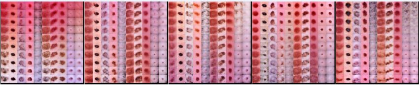
There have been many methods proposed in literature [1, 14, 19, 23, 29]
that explain predictions of deep neural networks based on the relevance of
different features or pixels/superpixels for an image. Recently, an approach
called contrastive explanations method (CEM) [6] was proposed which highlights
not just correlations or relevances but also features that are minimally sufficient to
justify a classification, referred to as pertinent positives (PPs). CEM additionally
outputs a minimal set of features, referred to as pertinent negatives (PNs), which
when made non-zero or added, alter the classification and thus should remain
absent in order for the original classification to prevail. For example, when
justifying the classification of a handwritten image of a 3, the method will
identify a subset of non-zero or on-pixels within the 3 which by themselves
are sufficient for the image to be predicted as a 3 even if all other pixels are
turned off (that is, made zero to match background). Moreover, it will identify
a minimal set of off-pixels which if turned on (viz. a horizontal line of pixels at
the right top making the 3 look like a 5) will alter the classification. Such forms
of explanations are not only common in day-to-day social interactions (viz. the
twin without the scar) but are also heavily used in fields such as medicine and
criminology [6]. [18] notably surveyed 250 papers in social science and philosophy
and found contrastive explanations to be among the most important for human
explanations.
    To identify PNs, addition is easy to define for grayscale images where a pixel
with a value of zero indicates no information and so increasing its value towards
1 indicates addition. However, for colored images with rich structure, it is not
clear what is a “no information" value for a pixel and consequently what does one
mean by addition. Defining addition in a naive way such as simply increasing
the pixel or red-green-blue (RGB) channel intensities can lead to uninterpretable
images as the relative structure may not be maintained with the added portion
being not necessarily interpretable. Moreover, even for grayscaled images just
increasing values of pixels may not lead to humanly interpretable images nor is
there a guarantee that the added portion can be interpreted even if the overall
image is realistic and lies on the data manifold.
    In this paper, we overcome these limitations by defining “addition" in a novel
way which leads to realistic images with the additions also being interpretable.
This work is an important contribution toward explaining black-box model
predictions because it is applicable to a large class of data sets (whereas [6] was
very limited in scope). To showcase the general applicability of our method to
various settings, we first experiment with CelebA [17] where we apply our method
to a data manifold learned using a generative adversarial network (GAN) [8]
trained over the data and by building attribute classifiers for certain high-level
concepts (viz. lipstick, hair color) in the dataset. We create realistic images with
interpretable additions. Our second experiment is on ISIC Lesions [5, 31] where
the data manifold is learned using a variational autoencoder (VAE) [15] and
certain (interpretable) latent factors (as no attributes are available) are used to
create realistic images with, again, interpretable additions. Latent factors are
also learned for a third experiment with Fashion-MNIST [34].
    Please note our assumption that high-level interpretable features can be

                                          2
learned if not given is not the subject of this paper and has been addressed in
multiple existing works, e.g., [4,13]. A key benefit to disentangled representations
is interpretability as discussed in [15]. The practicality and interpretability of
disentenagled features is further validated here by its use in the ISIC Lesions
and Fashion-MNIST datasets.
    The three usecases show that our method can be applied to colored as well as
grayscale images and to datasets that may or may not have high level attributes.
It is important to note that our goal is not to generate interpretable models that
are understood by humans, but rather to explain why a fixed model outputs a
particular prediction. We conducted a human study which concludes that our
method offers superior explanations compared to other methods, in particular
because our contrastive explanations go beyond visual explanations, which is
key to human comprehension.

2    Related Work
There have been many methods proposed in literature that aim to explain reasons
for their decisions. These methods may be globally interpretable – rule/decision
lists [30, 33], or exemplar based – prototype exploration [9, 12], or inspired by
psychometrics [10] or interpretable generalizations of linear models [3]. Moreover,
there are also works that try to formalize interpretability [7].
    A survey by [19] mainly explores two methods for explaining decisions of
neural networks: i) Prototype selection methods [21,22] that produce a prototype
for a given class, and ii) Local explanation methods that highlight relevant input
features/pixels [1, 14, 25, 28]. Belonging to this second type are multiple local
explanation methods that generate explanations for images [23, 24, 29] and some
others for NLP applications [16]. There are also works [13] that highlight higher
level concepts present in images based on examples of concepts provided by
the user. These methods mostly focus on features that are present, although
they may highlight negatively contributing features to the final classification. In
particular, they do not identify concepts or features that are minimally sufficient
to justify the classification or those that should be necessarily absent to maintain
the original classification. There are also methods that perturb the input and
remove features [27] to verify their importance, but these methods can only
evaluate an explanation and do not find one.
    Recently, there have been works that look beyond relevance. In [26], the
authors try to find features that, with almost certainty, indicate a particular
class. These can be seen as global indicators for a particular class. Of course,
these may not always exist for a dataset. There are also works [35] that try to
find stable insight that can be conveyed to the user in a (asymmetric) binary
setting for medium-sized neural networks. The most relevant work to our current
endevour is [6] and, as mentioned before, it cannot be directly applied when it
comes to explaining colored images or images with rich structure.

                                         3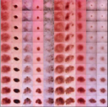
3     Methodology
We now describe the methodology for generating contrastive explanations for
images. We first describe how to identify PNs, which involves the key contribution
of defining “addition" for colored images in a meaningful way. We then describe
how to identify PPs, which also utilizes this notion of adding attributes. Finally,
we provide algorithmic details for solving the optimization problems in Algorithm
1.
    We first introduce some notation. Let X denote the feasible input space
with (x0 , t0 ) being an example such that x0 ∈ X and t0 is the predicted label
obtained from a neural network classifier. Let S denote the set of superpixels
that partition x0 with M denoting a set of binary masks which when applied to
x0 produce images M(x0 ) by selecting the corresponding superpixels from S.
Let Mx denote the mask corresponding to image x = Mx (x0 ).
    If D(.) denotes the data manifold (based on GAN or VAE), then let z
denote the latent representation with zx denoting the latent representation
corresponding to input x such that x = D(zx ). Let k denote the number of
(available or learned) interpretable features (latent or otherwise) which represent
meaningful concepts (viz. moustache, glasses, smile) and let gi (.), ∀i ∈ {1, ..., k},
be corresponding functions acting on these features with higher values indicating
presence of a certain visual concept while lower values indicating its absense.
For example, CelebA has different high-level (interpretable) features for each
image such as whether the person has black hair or high cheekbones. In this
case, we could build binary classifiers for each of the features where a 1 would
indicate presence of black hair or high cheekbones, while a zero would mean
its absense. These classifiers would be the gi (.) functions. On the other hand,
for datasets with no high-level interpretable features, we could find latents by
learning disentangled representations and choose those latents (with ranges) that
are interpretable. Here the gi functions would be an identity map or negative
identity map depending on which direction adds a certain concept (viz. light
colored lesion to a dark lesion). We note that these attribute functions could be
used as latent features for the generator in a causal graph (e.g., [20]), or given a
causal graph for the desired attributes, we could learn these functions from the
architecture in [20].
    Our procedure for finding PNs and PPs involves solving an optimization
problem over the variable δ which is the outputted image. We denote the
prediction of the model on the example x by f (x), where f (·) is any function
that outputs a vector of prediction scores for all classes, such as prediction
probabilities and logits (unnormalized probabilities) that are widely used in
neural networks.

3.1    Pertinent Negatives (PNs)
To find PNs, we want to create a (realistic) image that lies in a different class
than the original image but where we can claim that we have (minimally) “added"
things to the original image without deleting anything to obtain this new image.

                                          4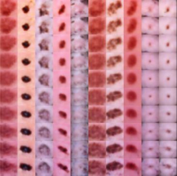
Algorithm 1 Contrastive Explanations Method using Monotonic Attribute
Functions (CEM-MAF)
  Input: Example (x0 , t0 ), latent representation of x0 denoted zx0 , neural
  network classification model f (.), set of (binary) masks M, and k monotonic
  feature functions g = {g1 (.), ..., gk (.)}.
  1) Solve (1) on example (x0 , t0 ) and obtain δ PN as the minimizing Pertinent
  Negative.
  2) Solve (2) on example (x0 , t0 ) and obtain δ PP as the minimizing Pertinent
  Positive.
  return δ PN and δ PP . {Code provided in supplement.}

If we are able to do this, we can say that the things that were added, which we
call PNs, should be necessarily absent from the original image in order for its
classification to remain unchanged.
     The question is how to define “addition" for colored or images with rich
structure. In [6], the authors tested on grayscale images where intuitively it is
easy to define addition as increasing the pixel values towards 1. This, however,
does not generalize to images where there are multiple channels (viz. RGB) and
inherent structure that leads to realistic images, and where simply moving away
from a certain pixel value may lead to unrealistic images. Moreover, addition
defined in this manner may be completely uninterpretable. This is true even
for grayscale images where, while the final image may be realistic, the addition
may not be. The other big issue is that for colored images the background
may be any color which indicates no signal and object pixels which are lower
in value in the original image if increased towards background will make the
object imperceptible in the new image, although the claim would be that we
have “added" something. Such counterintuitive cases arise for complex images if
we maintain their definition of addition.
     Given these issues, we define addition in a novel manner. To define addition
we assume that we have high-level interpretable features available for the dataset.
Multiple public datasets [17, 36] have high-level interpretable features, while
for others such features can be learned using unsupervised methods such as
disentangled representations [15] or supervised methods where one learns concepts
through labeled examples [13]. Given k such features, we define functions
gi (.), ∀i ∈ {1, ..., k}, as before, where in each of these functions, increasing value
indicates addition of a concept. Using these functions, we define addition as
introducing more concepts into an image without deleting existing concepts.
Formally, this corresponds to never decreasing the gi (.) from their original values
based on the input image, but rather increasing them. However, we also want a
minimal number of additions for our explanation to be crisp and so we encourage
as few gi () as possible to increase in value (within their allowed ranges) that will
result in the final image being in a different class. We also want the final image
to be realistic and that is why we learn a manifold D on which we perturb the
image, as we want our final image to also lie on it after the necessary additions.

                                          5
This gives rise to the following optimization problem:
                    X
            min γ      max{gi (x0 ) − gi (D(zδ )), 0} + βkg (D(zδ )) k1
              δ∈X
                       i
                    − c · min{max[f (δ)]i − [f (δ)]t0 , κ}
                               i6=t0

                    + ηkx0 − D(zδ )k22 + νkzx0 − zδ k22 .                             (1)
The first two terms in the objective function here are the novelty for PNs. The
first term encourages the addition of attributes where we want the gi (.)s for the
final image to be no less than their original values. The second term encourages
minimal addition of interpretable attributes. The third term is the PN loss
from [6] and encourages the modified example δ to be predicted as a different
class than t0 = arg maxi [f (x0 )]i , where [f (δ)]i is the i-th class prediction score of
δ. The hinge-like loss function pushes the modified example δ to lie in a different
class than x0 . The parameter κ ≥ 0 is a confidence parameter that controls the
separation between [f (δ)]t0 and maxi6=t0 [f (δ)]i . The fourth (η > 0) and fifth
terms (ν > 0) encourage the final image to be close to the original image in the
input and latent spaces. In practice, one could have a threshold for each of the
gi (.), where only an increase in values only beyond that threshold would imply a
meaningful addition. The advantage of defining addition in this manner is that
not only are the final images interpretable, but so are the additions, and we can
clearly elucidate which (concepts) should be necessarily absent to maintain the
original classification.

3.2     Pertinent Positives (PPs)
To find PPs, we want to highlight a minimal set of important pixels or superpixels
which by themselves are sufficient for the classifier to output the same class as the
original example. More formally, for an example image x0 , our goal is to find an
image δ ∈ M(x0 ) such that argmaxi [Pred(x0 )]i = argmaxi [Pred(δ)]i (i.e. same
prediction), with δ containing as few superpixels and interpretable concepts from
the original image as possible. This leads to the following optimization problem:
                           X
                  min γ        max{gi (δ) − gi (x0 ), 0} + βkMδ k1
                 δ∈M(x0 )
                               i
                            − c · min{[f (δ)]t0 − max[f (δ)]i , κ}.                   (2)
                                                   i6=t0

The first term in the objective function here is the novelty for PPs and penalizes
the addition of attributes since we seek a sparse explanation. The last term is the
PP loss from [6] and is minimized when [f (δ)]t0 is greater than maxi6=t0 [f (δ)]i by
at least κ ≥ 0, which is a margin/confidence parameter. Parameters γ, c, β ≥ 0
are the associated regularization coefficients.
    In the above formulation, we optimize over superpixels which of course
subsumes the case of just using pixels. Superpixels have been used in prior
works [25] to provide more interpretable results on image datasets and we allow
for this more general option.

                                            6
Orig.   yng, ml,       yng, fml,   yng, fml,    yng, fml,   old, ml,    Mela                 B. Cell      B. Kera    Vasc.
Class    smlg            smlg      not smlg     not smlg    not smlg   -noma      Nevus      Carc.         -tosis    Lesion
Orig.

 PN     old, fml,      old, fml,    yng, ml,    yng, fml,   old, ml,             Vasc.                     Mela     Bas. Cell
Class     smlg           smlg       not smlg     smlg        smlg      Nevus     Lesion      Nevus        -noma      Carc.
 PN

        +brwn hr,                   +single                                                                           more
                                                +makeup
        +makeup,          +oval     hair clr,               +cheek               rounder,   rounder,                  oval,
 PN                                              +oval                 rounder                            darker
Expl.    +bangs            face      -bangs       face      -bones                smaller    lighter                 smaller

 PP
LIME

 Grad
-CAM

                          (a) CelebA dataset                                          (b) ISIC Lesion dataset

                    Figure 1: CEM-MAF examples on (a) CelebA and (b) ISIC Lesions, both using
                    segmentation with 200 superpixels. Abbreviations are: Orig. for Original, PN
                    for Pertinent Negative, P for Pertinent Positive, and Expl. for Explanation.
                    In (a), change from original class prediction is in bold in PN class prediction.
                    Abbreviations in class predictions are as follows: yng for young, ml for male, fml
                    for female, smlg for smiling. In (b), change from original prediction is based on
                    change in disentangled features.

                    3.3     Optimization Details
                    To solve for PNs as formulated in (1), we note that the L1 regularization
                    term is penalizing a non-identity and complicated function kg (D(zδ )) k1 of the
                    optimization variable δ involving the data manifold D, so proximal methods are
                    not applicable. Instead, we use 1000 iterations of standard subgradient descent
                    to solve (1). We find a PN by setting it to be the iterate having the smallest L2
                    distance kzx0 − zδ k2 to the latent code zx0 of x0 , among all iterates where the
                    prediction score of solution δ ∗ is at least [f (xo )]t0 .
                        To solve for PPs as formulated in (2), we first relax the binary mask Mδ
                    on superpixels to be real-valued (each entry is between [0, 1]) and then apply
                    the standard iterative soft thresholding algorithm (ISTA) (see [2] for various
                    references) that efficiently solves optimization problems with L1 regularization.
                    We run 100 iterations of ISTA in our experiments and obtain a solution Mδ∗
                    that has the smallest L1 norm and satisfies the prediction of δ ∗ being within
                    margin κ of [f (xo )]t0 . We then rank the entries in Mδ∗ according to their values
                    in descending order and subsequently add ranked superpixels until the masked
                    image predicts [f (xo )]t0 .

                                                              7
A discussion of hyperparameter selection is held to the Supplement.

4       Experiments
We next illustrate the usefulness of CEM-MAF on two image data sets -
CelebA [17] and ISIC Lesions [5, 31] (results on Fashion-MNIST [34] are in
the Supplement). These datasets cover the gamut of images having known versus
derived features. CEM-MAF handles each scenario and offers explanations that
are understandable by humans. These experiments exemplify the following
observations:
• PNs offer intuitive explanations given a set of interpretable monotonic attribute
  functions. In fact, our user study finds them to be the preferred form of
  explanation since describing a decision in isolation (viz. why is a smile a smile)
  using PPs, relevance, or heatmaps is not always informative.
• PPs offer better direction as to what is important for the classification versus
  too much direction by LIME (shows too many features) or too little direction
  by Grad-CAM (only focuses on smiles).

• PPs and PNs offer the guarantee of being 100% accurate in maintaining or
  changing the class respectively as seen in Table 1 versus LIME or Grad-CAM.
• Both proximity in the input and latent space along with sparsity in the addi-
  tions play an important role in generating good quality human-understandable
  contrastive explanations.

4.1     CelebA with Available High-Level Features
CelebA is a large-scale dataset of celebrity faces annotated with 40 attributes [17].

4.1.1    Setup
The CelebA experiments explain an 8-class classifier learned from the following
binary attributes: Young/Old, Male/Female, Smiling/Not Smiling. We train a
Resnet50 [11] architecture to classify the original CelebA images. We selected
the following 11 attributes as our {gi } based on previous studies [15] as well as
based on what might be relevant for our class labels: High Cheekbones, Narrow
Eyes, Oval Face, Bags Under Eyes, Heavy Makeup, Wearing Lipstick, Bangs,
Gray Hair, Brown Hair, Black Hair and Blonde Hair. Note that this list does
not include the attributes that define the classes because an explanation for
someone that is smiling which simply says they are smiling would not be useful.
See Supplement for details on training these attribute functions and the GAN
used for generation.

                                         8
Table 1: Quantitative comparison of CEM-MAF, LIME, and Grad-CAM on the
CelebA and ISIC Lesions datasets. Results for Fashion-MNIST with similar
patterns can be found in the Supplement.

                                            # PP    PP      PP
               Dataset      Method          Feat    Acc    Corr
                           CEM-MAF           16.0   100    -.742
                CelebA       LIME            75.1    30    .035
                           Grad-CAM          17.6    30    .266
                           CEM-MAF           66.7   100    -.976
                 ISIC
                Lesions      LIME           108.3   100    -.986
                           Grad-CAM          95.6    50    -.772

4.1.2   Observations
Results on five images are exhibited in Figure 1 (a) using a segmentation into
200 superpixels (more examples in Supplement). The first two rows show the
original class prediction followed by the original image. The next two rows
show the pertinent negative’s class prediction and the pertinent negative image.
The fourth row lists the attributes that were modified in the original, i.e., the
reasons why the original image is not classified as being in the class of the
pertinent negative. The next row shows the pertinent positive image, which
combined with the PN, gives the complete explanation. The final two rows
illustrate different explanations that can be compared with the PP: one derived
from locally interpretable model-agnostic explanations (LIME) [25] followed by a
gradient-based localized explanation designed for CNN models (Grad-CAM) [24].
    First consider class explanations given by the PPs. Age seems to be captured
by patches of skin, sex by patches of hair, and smiling by the presence or absence
of the mouth. One might consider the patches of skin to be used to explain
young versus old. PPs capture a part of the smile for those smiling, while leave
out the mouth for those not smiling. Visually, these explanations are simple
(very few selected features) and useful although they require human analysis. In
comparison, LIME selects many more features that are relevant to the prediction,
and while also useful, requires even more human intervention to explain the
classifier. Grad-CAM, which is more useful for discriminative tasks, seems to
focus on the mouth and does not always find a part of the image that is positively
relevant to the prediction.
    A performance comparison of PPs between CEM-MAF, LIME, and Grad-
CAM is given in Table 1. Across colored images, CEM-MAF finds a much
sparser subset of superpixels than LIME and is guaranteed to have the same
prediction as the original image. Both LIME and Grad-CAM select features for
visual explanations that often have the wrong prediction (low PP accuracy). A
third measure, PP Correlation, measures the benefit of each additional feature
by ranking the prediction scores after each feature is added (confidence in the

                                        9
prediction should increase) and correlating with the expected ranks (perfect
correlation here would give -1). Order for LIME was determined by classifier
weights while order for Grad-CAM was determined by colors in the corresponding
heatmaps. CEM-MAF is best or on par at selecting features that increase
confidence.
More intuitive explanations are offered by the pertinent negatives in Figure
1. The first PN changes a young, smiling, male into an old, smiling, female
by adding a second hair color, makeup, and bangs. Younger age more likely
corresponds to a single hair, and being male is explained by a lack of makeup or
bangs, more associated with females. Another way to explain young age is the
absence of an oval face in the second column. The third PN changes a female
into a male, and the female is explained by the absence of a single hair color
(in fact, she has black hair with brown highlights) and the presence of bangs.
While the presence of bangs is intuitive, it is selected because our constraints of
adding features to form PNs can be violated due to enforcing the constraints
with regularization. The last two columns explain a face not smiling by the
absence of high cheekbones or the absence of an oval face (since your face can
become more oval when you raise your cheekbones).
Note that the first example where the male was changed to a female in the
PN was obtained by regularizing only the latent representation proximity. Our
framework allows for different regularizations, and in fact, regularizing sparsity
in the number of attributes for this example results in a PN with only a single,
rather than three, added attributes classified as a young male that is not smiling
(image in Supplement).
4.2 Skin Lesions with Learned Disentangled Features
The International Skin Imaging Collaboration (ISIC) Archive (https://challenge2018.
isic-archive.com/) is a large-scale image dataset consisting of dermoscopic
(special photographic technique for removing surface reflections) images of skin
lesions [5, 31]. Descriptions of the seven different types of lesions can be found in
the Supplement.
4.2.1 Setup
For ISIC Lesions, we explain a 7-class classifier trained on a Resnet9 architecture
(classes such as melanoma, nevus, etc.). As with CelebA, we train a VAE to
generate realistic images for PNs. However, this data does not have annotated
features as in CelebA, so we learn the features using disentanglement following
a recent variant of VAE called DIP-VAE [15] (see Supplement for more details).
We can then use these disentangled latent features in lieu of the ground
truth attributes. Based on what might be relevant to the categories of skin
lesions, we use ten dimensions from the latent code as attributes, corresponding
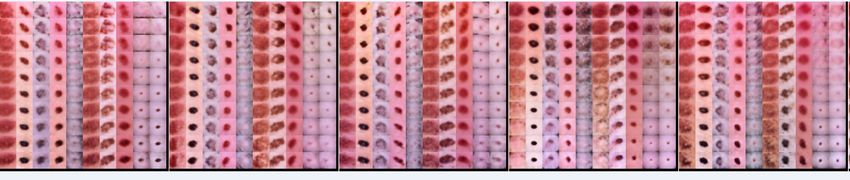
to size, roundness, darkness, and border definition. Figure 2 visualizes features
corresponding to increasing size and shape change from circular to oval as the
10Increasing Size Circular to Oval Shape
Figure 2: Qualitative results for disentanglement of ISIC Lesions images. Full
visualization is in the Supplement.
features increase. A visualization of all disentangled features, ISIC Lesions and
Fashion-MNIST, can be found in the Supplement.
4.2.2 Observations
Results on five images are exhibited in Figure 1 (b), also using a segmentation
into 200 superpixels (more examples in the Supplement). Rows here are the
same as described above for CelebA. Explanations for the PPs can be determined
using descriptions of the lesions. The first PP for an image of Melanoma leaves
parts of the lesion displaying two different colors, black and brown (these lesions
usually do not have a single solid color). The third PP of Basal Cell Carcinoma
highlights the pink and skin color associated with the most common type of
such lesions (and removes the border meaning the prediction does not focus
on the border). LIME highlights similar areas, while using more superpixels.
Grad-CAM mostly does not highlight specific areas of the lesions, but rather
the entire lesion. Grad-CAM removes the brown part of the first Melanoma and
the resulting prediction is incorrect (Melanoma usually does not have a single
solid color). Note that Nevus lesion PPs contain a single superpixel due to heavy
dataset bias for this class.
The contrastive explanations offered by the PNs offer much more intuition.
For example, the first lesion is classified as a Melanoma because it is not rounder,
in which case it would be classified as a Nevus (the PN). In fact, Melanomas are
known to be asymmetrical due to the quick and irregular growth of cancer cells
in comparison to normal cells. In the fourth column, the Benign Keratosis lesion
is classified as such because it is not darker, in which case it would be classified
as a Melanoma (the darker center creates the multi-colored lesion associated
with Melanoma)
5 User Study
In order to further illustrate the usefulness of, and preference for, contrastive
explanations, we conducted a thorough user study comparing CEM-MAF, LIME,
and Grad-CAM. Our study assesses two questions: are the explanations useful
by themselves and whether or not an additional explanation would add to
11CEM-MAF vs Grad-CAM vs LIME
Standalone Rating Additional Value
3
Rating
2
1
0
CEM G−CAM LIME CEM G−CAM LIME
PN vs PP vs Grad-CAM vs LIME
Standalone Rating Additional Value
3
Rating
2
1
0
PN PP G−CAM LIME PN PP G−CAM LIME
Figure 3: User study results. Top figures compare CEM-MAF with Grad-CAM
(G-CAM) and LIME, where figure (left) rates the usefulness of explanations
while figure (right) rates additional value given one of the other explanations.
Bottom figures show similar ratings but separates CEM-MAF into PN and PP.
Error bars show standard error.
the usefulness of an initial explanation. LIME and Grad-CAM clearly have
usefulness as explanation methods, evidenced by previous literature. Contrastive
explanations offer different information that could be viewed as complimentary
to the visual explanations given by the other methods. Pertinent positives, while
also visual, have a specific meaning in highlighting a minimally sufficient part of
the image to obtain a classifier’s prediction, while LIME highlights significant
features using local linear classifiers and Grad-CAM highlights features that
attribute maximum change to the prediction. Each method provides different
information. Pertinent negatives illuminate a completely different aspect that is
known to be intuitive to humans [18], and importantly does not require humans
to interpret what is learned since the method outputs exactly what modifications
are necessary to change the prediction.
The study was conducted on Amazon Mechanical Turk using CelebA images.
A single trial of the study proceeds as follows. An original image is displayed
along with the model’s prediction in a sentence, e.g.,“The system thinks the
image shows a young male who is smiling." Under the image, one of the three
explanation methods, titled “Explanation 1" for anonymity, is displayed with a
brief description of the explanation, e.g. “The colored pixels highlight the parts
of the original image that may have contributed significantly to the system’s
recognition result." The question, “Is the explanation useful?", is posed next
to Explanation 1 along with five choices ranging from “I don’t understand
12the explanation" to “I understand the explanation and it helps me completely
understand what features the system used to recognize a young, male, who is
smiling" (the words for the prediction change per image).
After answering the first question, another image, titled “Explanation 2", is
displayed under the first explanation, again with a short blurb about what the
explanation exhibits. If the first explanation was LIME, the second explanation
would be CEM-MAF or Grad-CAM. The question posed next to this explanation
is “How much does adding the second explanation to the first improve your
understanding of what features the system used to recognize a young male who
is smiling?" There are five possible responses ranging from “None" to “Completes
my understanding." In a second survey, we ask the same questions for four
methods, where we separate CEM-MAF and pose the pertinent positive and
pertinent negative as two different explanations. A screenshot of a single trial
can be found at the end of the Supplement.
Each user in the study is required to spend at least 30 seconds reading a page
of instructions that gives examples of the three (or four) possible explanations
and explains what will be asked during the survey. Then each user proceeds
through 24 trials as described above. Each of the three methods is assigned to
both explanations 1 and 2 such that a user sees each of the six permutations four
times (the second survey with four explanations has twelve permutations that
are each seen twice). Each trial draws a random image from a batch of 76 images
for which we have ran all methods. As LIME requires tuning, we restrict LIME
to use the same number of superpixels as used in the pertinent positives for an
apples-to-apples comparison. Regarding demographics, we attempt to run the
survey over a population that is more likely to use the methods of this paper by
restricting job function of participants to Information Technology. Each survey
was taken by 100 different participants (200 total), 157 males vs 40 females
(remaining declined), with 81 people aged 30-39 (full age table in Supplement).
Results are displayed in Figure 3. The standalone ratings judge individual
usefulness of all explanation methods. CEM-MAF has a clear, albeit, slight
advantage in terms of usefulness over other methods, and when broken down, it
is apparent that the usefulness is driven more by the PN than the PP, which is on
par with Grad-CAM. The direct explanation that requires no human intervention
to interpret the explanation seems to be most useful (i.e., PNs directly output
via text what the explanation is whereas other methods require a human to
interpret what is understood visually). Given one explanation, the additional
value of offering a second explanation follows a similar pattern to the standalone
ratings. This means that users given a Grad-CAM or LIME explanation found
the contrastive explanation to offer more additional understanding than if they
were first given CEM-MAF followed by Grad-CAM or LIME. Note these results
are averaged, for example, with CEM-MAF as the second explanation, over all
trials with either Grad-CAM or LIME as the first explanation.
While CEM-MAF was observed as the most useful explanation, comments
made at the end of the survey suggest what has been mentioned earlier: each of
the different explanation methods have value. Such comments included “The
explanations were straightforward" and “I thought they were pretty accurate
13overall and helped in the decision making process". Other comments suggested
that there is still much variability in the success of explanation methods, e.g., “I
thought they were very unique and amazing to see. I thought the explanations
were usually a bit confused, but some were very advanced" and “The explanation
made sense to me, though I think some of them were lacking in complexity
and detail." Such comments also point out where contrastive explanations can
have major impact. For example, since PP’s dictate, by definition, when a
classifier requires very little information to make its prediction (i.e., require
“little complexity and detail"), they can be used to locate classifiers that should
be reassessed prior to deployment.
6 Discussion
In this paper, we leveraged high-level features that were readily available (viz.
CelebA) as well as used generated ones (viz. ISIC Lesions and Fashion-MNIST)
based on unsupervised methods to produce contrastive explanations. As men-
tioned before, one could also learn interpretable features in a supervised manner
as done in [13] which we could also use to generate such explanations. Regarding
learning the data manifold, it is important to note that we do not need a global
data manifold to create explanations; a good local data representation around the
image should be sufficient. Thus, for datasets where building an accurate global
representation may be hard, a good local representation (viz. using conditional
GANs) should make it possible to generate high quality contrastive explanations.
Several future directions are motivated by the user study. Extracting text to
describe highlighted aspects of visual explanations (PP, LIME, and Grad-CAM)
could better help their understanding by humans. As previously mentioned, an
important feature of contrastive explanations is that they can be used to identify
classifiers that should not be trusted. PP’s composed of two superpixels in our
CelebA experiments could identify examples where the classifier requires little
relevant information, and hence might not be operating in a meaningful way.
The study reinforced this concept because users found visual explanations with
few superpixels to be less useful. Studying this relationship between human
trust and contrastive explanations is an interesting direction.
In summary, we have proposed a method to create contrastive explanations
for image data with rich structure. The key novelty over previous work is how we
define addition, which leads to realistic images where added information is easy
to interpret (e.g., added makeup). Our results showcase that using pertinent
negatives might be the preferred form of explanation where it is not clear why
a certain entity is what it is in isolation (e.g. based on relevance or pertinent
positives), but could be explained more crisply by contrasting it to another entity
that closely resembles it (viz. adding high cheekbones to a face makes it look
smiling).
14References
[1] Sebastian Bach, Alexander Binder, Grégoire Montavon, Frederick Klauschen,
Klaus-Robert Müller, and Wojciech Samek. On pixel-wise explanations for
non-linear classifier decisions by layer-wise relevance propagation. PloS one,
10(7):e0130140, 2015.
[2] Amir Beck and Marc Teboulle. A fast iterative shrinkage-thresholding
algorithm for linear inverse problems. SIAM journal on imaging sciences,
2(1):183–202, 2009.
[3] Rich Caruana, Yin Lou, Johannes Gehrke, Paul Koch, Marc Sturm, and
Noemie Elhadad. Intelligible models for healthcare: Predicting pneumonia
risk and hospital 30-day readmission. In KDD 2015, pages 1721–1730, New
York, NY, USA, 2015. ACM.
[4] Xi Chen, Yan Duan, Rein Houthooft, John Schulman, Ilya Sutskever, and
Pieter Abbeel. Infogan: Interpretable representation learning by information
maximizing generative adversarial nets. In Advances in Neural Information
Processing Systems, 2016.
[5] N. Codella, V. Rotemberg, P. Tschandl, M. E. Celebi, S. Dusza, D. Gut-
manand B. Helba, A. Kalloo, K. Liopyris, M. Marchetti, H. Kittler, and
A. Halpern. Skin lesion analysis toward melanoma detection 2018: A
challenge hosted by the international skin imaging collaboration (isic). In
https://arxiv.org/abs/1902.03368, 2018.
[6] Amit Dhurandhar, Pin-Yu Chen, Ronny Luss, Chun-Chen Tu, Paishun
Ting, Karthikeyan Shanmugam, and Payel Das. Explanations based on
the missing: Towards contrastive explanations with pertinent negatives. In
NeurIPS 2018, 2018.
[7] Amit Dhurandhar, Vijay Iyengar, Ronny Luss, and Karthikeyan Shan-
mugam. Tip: Typifying the interpretability of procedures. arXiv preprint
arXiv:1706.02952, 2017.
[8] I. Goodfellow, Y. Bengio, and A. Courville. Deep Learning. MIT Press,
2016.
[9] Karthik Gurumoorthy, Amit Dhurandhar, and Guillermo Cecchi. Protodash:
Fast interpretable prototype selection. arXiv preprint arXiv:1707.01212,
2017.
[10] Tsuyoshi Idé and Amit Dhurandhar. Supervised item response models for
informative prediction. Knowl. Inf. Syst., 51(1):235–257, April 2017.
[11] Shaoqing Ren Kaiming He, Xiangyu Zhang and Jian Sun. Deep residual
learning for image recognition. In CVPR 2016, June 2016.
15[12] Been Kim, Rajiv Khanna, and Oluwasanmi Koyejo. Examples are not
enough, learn to criticize! criticism for interpretability. In In Advances of
Neural Inf. Proc. Systems, 2016.
[13] Been Kim, Martin Wattenberg, Justin Gilmer, Carrie Cai, James Wexler,
Fernanda Viegas, and Rory Sayres. Interpretability beyond feature attribu-
tion: Quantitative testing with concept activation vectors. Intl. Conf. on
Machine Learning, 2018.
[14] Pieter-Jan Kindermans, Kristof T. Schütt, Maximilian Alber, Klaus-Robert
Müller, Dumitru Erhan, Been Kim, and Sven Dähne. Learning how to
explain neural networks: Patternnet and patternattribution. In Intl. Con-
ference on Learning Representations (ICLR), 2018.
[15] Abhishek Kumar, Prasanna Sattigeri, and Avinash Balakrishnan. Variational
inference of disentangled latent concepts from unlabeled observations. Intl.
Conf. on Learning Representations, 2017.
[16] Tao Lei, Regina Barzilay, and Tommi Jaakkola. Rationalizing neural
predictions. arXiv preprint arXiv:1606.04155, 2016.
[17] Ziwei Liu, Ping Luo, Xiaogang Wang, and Xiaoou Tang. Deep learning face
attributes in the wild. In ICCV 2015, December 2015.
[18] Tim Miller. Contrastive explanation: A structural-model approach. CoRR,
abs/1811.03163, 2018.
[19] Grégoire Montavon, Wojciech Samek, and Klaus-Robert Müller. Methods
for interpreting and understanding deep neural networks. Digital Signal
Processing, 2017.
[20] Alexandros G. Dimakis Murat Kocaoglum Christopher Snyder and Sriram
Vishwanath. Causalgan: Learning causal implicit generative models with
adversarial training. In ICLR 2018, 2018.
[21] Anh Nguyen, Alexey Dosovitskiy, Jason Yosinski, Thomas Brox, and Jeff
Clune. Synthesizing the preferred inputs for neurons in neural networks via
deep generator networks. In NIPS, 2016.
[22] Anh Nguyen, Jason Yosinski, and Jeff Clune. Multifaceted feature visual-
ization: Uncovering the different types of features learned by each neuron
in deep neural networks. arXiv preprint arXiv:1602.03616, 2016.
[23] Jose Oramas, Kaili Wang, and Tinne Tuytelaars. Visual explanation by in-
terpretation: Improving visual feedback capabilities of deep neural networks.
In arXiv:1712.06302, 2017.
[24] Abhishek Das Ramakrishna Vedantam Devi Parikh Ramprasaath R. Sel-
varaju, Michael Cogswell and Dhruv Batra. Grad-cam: Visual explanations
from deep networks via gradient-based localization. In ICCV, October 2017.
16[25] Marco Ribeiro, Sameer Singh, and Carlos Guestrin. "why should i trust
you?” explaining the predictions of any classifier. In KDD 2016, 2016.
[26] Marco Tulio Ribeiro, Sameer Singh, and Carlos Guestrin. Anchors: High-
precision model-agnostic explanations. In AAAI 2018, 2018.
[27] Wojciech Samek, Alexander Binder, Grégoire Montavon, Sebastian La-
puschkin, and Klaus-Robert Müller. Evaluating the visualization of what a
deep neural network has learned. In IEEE TNNLS, 2017.
[28] Su-In Lee Scott Lundberg. Unified framework for interpretable methods.
In NIPS 2017, 2017.
[29] Karen Simonyan, Andrea Vedaldi, and Andrew Zisserman. Deep inside
convolutional networks: Visualising image classification models and saliency
maps. CoRR, abs/1312.6034, 2013.
[30] Guolong Su, Dennis Wei, Kush Varshney, and Dmitry Malioutov.
Interpretable two-level boolean rule learning for classification. In
https://arxiv.org/abs/1606.05798, 2016.
[31] P. Tschandl, C. Rosendahl, and H. Kittler. The ham10000 dataset, a large
collection of multi-source dermatoscopic images of common pigmented skin
lesions. Sci. Data, 5, 2018.
[32] Kush Varshney. Engineering safety in machine learning. In
https://arxiv.org/abs/1601.04126, 2016.
[33] Fulton Wang and Cynthia Rudin. Falling rule lists. In In AISTATS, 2015.
[34] Han Xiao, Kashif Rasul, and Roland Vollgraf. Fashion-mnist: a novel
image dataset for benchmarking machine learning algorithms. CoRR,
abs/1708.07747, 2017.
[35] Xin Zhang, Armando Solar-Lezama, and Rishabh Singh. Interpreting neural
network judgments via minimal, stable, and symbolic corrections. 2018.
https://arxiv.org/abs/1802.07384.
[36] Shi Qiu Xiaogang Wang Ziwei Liu, Ping Luo and Xiaoou Tang. Deepfashion:
Powering robust clothes recognition and retrieval with rich annotations. In
CVPR 2016, June 2016.
17Supplement
Note all model training for experiments is done using Tensorflow and Keras.
1 Hyperparameter selection for PN and PP
Finding PNs is done by solving (1) which has hyperparameters κ, γ, β, η, µ, c. The
confidence parameter κ is the user’s choice. We experimented with κ ∈ {0.5, 5.0}
and report results with κ = 5.0. We experimented with γ ∈ {1, 100} and
report results with γ = 100 which better enforces the constraint of only adding
attributes to a PN. The three hyperparameters β = 100, η = 1.0, ν = 1.0 were
fixed. Sufficient sparsity in attributes was obtained with this value of β but
further experiments increasing β could be done to allow for more attributes if
desired. The results with selected η and ν were deemed realistic there so there
was no need to further tune them. Note that CelebA PN experiments required
experimenting with β = 0 to remove the attribute sparsity regularization. The
last hyperparameter c was selected via the following search: Start with c = 1.0
and multiply c by 10 if no PN found after 1000 iterations of subgradient descent,
and divided by 2 if PN found. Then run the next 1000 iterations and update c
again. This search on c was repeated 9 times, meaning a total of 1000 × 9 = 9000
iterations of subgradient descent were run with all other hyperparameters fixed.
Finding PPs is done by solving (2) which has hyperparameters κ, γ, β, c.
Again, we experimented with κ ∈ {0.5, 5.0} and report results with κ = 5.0. We
experimented with γ ∈ {1, 100} and report results with γ = 100 for the same
reason as for PNs. The hyperparameter β = 0.1 because β = 100 as above was
too strong and did not find PPs with such high sparsity (usually allowing no
selection). The same search on c as described for PNs above was done for PPs,
except this means a total of 9 × 100 iterations of ISTA were run with all other
hyperparameters fixed to learn a single PP.
2 Additional CelebA Information
We here discuss how attribute classifiers were trained for CelebA, describe
the GAN used for generation, and provide additional examples of CEM-MAF.
CelebA datasets are available at http://mmlab.ie.cuhk.edu.hk/projects/
CelebA.html.
2.1 Training attribute classifiers for CelebA
For each of the 11 selected binary attributes, a CNN with four convolutional
layers followed by a single dense layer was trained on 10000 CelebA images with
Tensorflow’s SGD optimizer with Nesterov using learning rate=0.001, decay=1e-
6, and momentum=0.9. for 250 epochs. Accuracies of each classifiers are given
in Table 2.
18Table 2: CelebA binary attribute classifer accuracies on 1000 test images
Attribute Accuracy
High Cheekbones 84.5%
Narrow Eyes 78.8%
Oval Face 63.7%
Bags Under Eyes 79.3%
Heavy Makeup 87.9%
Wearing Lipstick 90.6%
Bangs 93.0%
Gray Hair 93.5%
Brown Hair 76.3%
Black Hair 86.5%
Blonde Hair 93.1%
2.2 GAN Information
Our setup processes each face as a 224 × 224 pixel colored image. A GAN was
trained over the CelebA dataset in order to generate new images that lie in
the same distribution of images as CelebA. Specifically, we use the pretrained
progressive GAN1 to approximate the data manifold of the CelebA dataset.
The progressive training technique is able to grow both the generator and
discriminator from low to high resolution, generating realistic human face images
at different resolutions.
2.3 Additional CelebA Examples
Figure 4 (a) gives additional examples of applying CEM-MAF to CelebA. Similar
patterns can be seen with the PPs. CEM-MAF provides sparse explanations
highlighting a few features, LIME provides explanations (positively relevant
superpixels) that cover most of the image, and Grad-CAM focuses on the mouth
area.
3 Additional ISIC Lesions Information
We here discuss what the different types of lesions in the ISIC dataset are,
how disentangled features were learned for ISIC lesions, and provide additional
examples of CEM-MAF. The ISIS Lesions dataset is available at https://
challenge2018.isic-archive.com/.
1 https://github.com/tkarras/progressive_growing_of_gans
19Original old, fml, yng, fml, yng, fml, yng, ml, yng, fml, A. Kera, B. Kera, Vasc.,
Class Pred not smlg smlg smlg smlg not smlg Nevus Nevus -tosis -tosis Lesion
Original
Pert. Neg. yng, fml, yng, fml, yng, ml, yng, ml, old, fml, Mela B. Kera, B. Cell,
Class Pred smlg not smlg smlg not smlg smlg -noma -tosis Nevis Carc. Nevis
Pertinent
Negative
Pertinent
Positive
LIME
Grad-CAM
(a) CelebA dataset (b) ISIC Lesion dataset
Figure 4: Additional CEM-MAF examples on CelebA (a) and ISIC Lessions (b)
using segmentation with 200 superpixels. Change from original class prediction
is in bold in PN class prediction for CelebA. Abbreviations in class predictions
are as follows: yng for young, ml for male, fml for female, smlg for smiling. For
ISIS Lesions, change from original prediction is based on change in disentangled
features.
3.1 Lesion Descriptions
The ISIC dataset is composed of dermoscopic images of lesions classified into the
following seven categories: Melanoma, Melanocytic Nevus, Basal Cell Carcinoma,
Actinic Keratosis, Benign Keratosis, Dermatofibroma, and Vascular Lesions.
Information about these categories is available at https://challenge2018.
isic-archive.com/ but we give some key information about these lesions
below. All description were obtained from www.healthline.com/health.
Melanoma: Cancerous mole, asymmetrical due to cancer cells growing more
quickly and irregularly than normal cells, fuzzy border, different shades of same
color or splotches of different color (but not one solid color). Many different
tests to diagnose the stage of cancer.
Melanocytic Nevus: Smooth, round or oval-shaped mole. Usually raised,
single or multi-colored, might have hairs growing out. Pink, tan, or brown.
Might need biopsy to rule out skin cancer.
Basal Cell Carcinoma: At least 5 types, pigmented (brown, blue, or black
lesion with translucent and raised border), superficial (reddish patch on the
skin, often flat and scaly, continues to grow and often has a raised edge),
nonulcerative (bump on the skin that is white, skin-colored, or pink, often
translucent, with blood vessels underneath that are visible, most common type of
BCC), morpheaform (least common type of BCC, typically resembles a scarlike
20lesion with a white and waxy appearance and no defined border), basosquamous
(extremely rare).
Actinic Keratosis: Typically flat, reddish, scale-like patch often larger than
one inch. Can start as firm, elevated bump, or lump. Skin patch can be brown,
tan, gray, or pink. Visual diagnosis, but skin biopsy necessary to rule out change
to cancer.
Benign Keratosis: Starts as small, rough, area, usually round or oval-shaped.
Usually brown, but can be yellow, white, or black. Usually diagnosed by eye.
Dermatofibroma: Small, round noncancerous growth, different layers. Usually
firm to the touch. Usually a visual diagnosis.
Vascular Lesions: *Too many types to list.
3.2 Learning Disentangled Features for ISIC Lesions
Our setup processes each item as a 128 × 128 pixel color image. As with
many real-world scenarios, ISIC Lesion samples come without any supervision
about the generative factors or attributes. For such data, we can rely on
latent generative models such as VAE that aim to maximize the likelihood of
generating new examples that match the observed data. VAE models have a
natural inference mechanism baked in and thus allow principled enhancement
in the learning objective to encourage disentanglement in the latent space. For
inferring disentangled factors, inferred prior or expected variational posterior
should be factorizable along its dimensions. We use a recent variant of VAE
called DIP-VAE [15] that encourages disentanglement by explicitly matching
the inferred aggregated posterior to the prior distribution. This is done by
matching the covariance of the two distributions which amounts to decorrelating
the dimensions of the inferred prior. Table 3 details the architecture for training
DIP-VAE on ISIC Lesions.
Figure 5 shows the disentanglement in these latent features by visualizing the
VAE decoder’s output for single latent traversals (varying a single latent between
[−3, 3] while keeping others fixed). For example, we can see that increasing the
value of the third dimension (top row) of the latent code corresponds to changing
from circular to oval while increasing the value of the fourth dimension (top row)
corresponds to decreasing size.
Table 3: Details of the model architecture used for training DIP-VAE [15] on
ISIC Lesions.
Architecture
Input 16384 (flattened 128x128x1)
Encoder Conv 32x4x4 (stride 2), 32x4x4 (stride 2),
64x4x4 (stride 2), 64x4x4 (stride 2), FC 256.
ReLU activation
Latents 32
Decoder Deconv reverse of encoder. ReLU activation.
Gaussian
21Figure 5: Qualitative results for disentanglement in the ISIC Lesions dataset.
The figure shows the DIP-VAE decoder’s output for single latent traversals
(varying a single latent between [−3, 3] while keeping others fixed). Each row
show 5 unique features separated by bold black lines.
4 Fashion-MNIST with Disentangled Features
Fashion-MNIST is a large-scale image dataset of various fashion items (e.g.,
coats, trousers, sandals). We here discuss how disentangled features were
learned for Fashion-MNIST, how classifiers were trained, and pro- vide ad-
ditional examples of CEM-MAF. Fashion-MNIST datasets are available at
https://github.com/zalandoresearch/ fashion-mnist.
4.0.1 Learning Disentangled Features for Fashion-MNIST
Two datasets are created as subsets of Fashion-MNIST, one for clothes (tee-shirts,
trousers, pullovers, dresses, coats, and shirts) and one for shoes (sandals, sneakers,
and ankleboots). Our setup processes each item as a 28 × 28 pixel grayscale
image. Again, a VAE was trained to learn the Fashion-MNIST manifold, and
we again learn the features using DIP-VAE due to a lack of annotated features.
Table 4 details the architecture for training DIP-VAE on Fashion-MNIST.
Based on what might be relevant to the clothes and shoes classes, we use
four dimensions from the latent codes corresponding to sleeve length, shoe mass,
heel length and waist size. Given these attributes, we learn two classifiers, one
with six classes (clothes) and one with three classes (shoes).
Figure 6 shows the disentanglement in these latent features by visualizing the
VAE decoder’s output for single latent traversals (varying a single latent between
[−3, 3] while keeping others fixed). For example, we can see that increasing the
value of the second dimension z2 of the latent code corresponds to increasing
sleeve length while increasing the value of the third dimension z3 corresponds to
adding more material on the shoe.
22Table 4: Details of the model architecture used for training DIP-VAE [15] on
Fashion-MNIST.
Architecture
Input 784 (flattened 28x28x1)
Encoder FC 1200, 1200. ReLU activation.
Latents 16
Decoder FC 1200, 1200, 1200, 784. ReLU
activation.
Optimizer Adam (lr = 1e-4) with mse loss
Figure 6: Qualitative results for disentanglement in Fashion MNIST dataset.
The figure shows the DIP-VAE decoder’s output for single latent traversals
(varying a single latent between [−3, 3] while keeping others fixed). The title of
each image grid denotes the dimension of the latent code that was varied.
4.1 Training Fashion-MNIST classifiers
Two datasets are created as subsets of Fashion-MNIST, one for clothes (tee-
shirts, trousers, pullovers, dresses, coats, and shirts) and one for shoes (sandals,
sneakers, and ankleboots). We train CNN models for each of these subsets with
two convolutional layers followed by two dense layer to classify corresponding
images from original Fashion-MNIST dataset. See Table 5 for training details.
4.1.1 Observations
Results on ten clothes images and ten shoe images are shown in Figure 7 (a)
and (b), respectively. In order to make a fair comparison with CEM, we do not
segment the images but rather do feature selection pixel-wise. Note that CEM
does not do pixel selection for PPs but rather modifies pixel values.
Let us first look at the PPs. They are mostly sparse explanations and do not
give any visually intuitive explanations. Both LIME and Grad-CAM, by selecting
many more relevant pixels, offers a much more visually appealing explanation.
However, these explanations simply imply, for example, that the shirt in the first
row of Figure 7 (a) is a shirt because it looks like a shirt. These two datasets
(clothes and shoes) are examples where the present features do not offer an
intuitive explanation. Table 1 again shows that CEM-MAF selects much fewer
23You can also read