Agricultural Productivity Growth and Its Determinants in South and Southeast Asian Countries - MDPI
←
→
Page content transcription
If your browser does not render page correctly, please read the page content below
sustainability

Article
Agricultural Productivity Growth and Its
Determinants in South and Southeast Asian Countries
Jianxu Liu 1,2 , Mengjiao Wang 2, * , Li Yang 1 , Sanzidur Rahman 1,3       and
Songsak Sriboonchitta 2
 1    Shandong University of Finance and Economics, Faculty of Economics, Jinan 250000, China;
      liujianxu1984@163.com (J.L.); liyang@sdufe.edu.cn (L.Y.); srahman@plymouth.ac.uk (S.R.)
 2    Faculty of Economics, Chiang Mai University, Chiang Mai 50200, Thailand; songsakecon@gmail.com
 3    Plymouth Business School, University of Plymouth, Drake Circus, Plymouth PL4 8AA, UK
 *    Correspondence: mengjiaow1991@163.com

 Received: 27 May 2020; Accepted: 16 June 2020; Published: 18 June 2020

 Abstract: Improving agricultural productivity is a priority concern in promoting the sustainable
 development of agriculture in developing countries. In this study, we first apply stochastic frontier
 analysis (SFA) to analyze the growth of agricultural total factor productivity (TFP) and its three
 components (technical change—TC, technical efficiency change—TEC and scale change—SC) in
 15 south and southeast Asian countries covering the period 2002 to 2016. Then, the determinants of
 agricultural TFP growth are identified using dynamic panel data models. The results reveal that the
 south and southeast Asian countries witnessed an overall decline in agricultural productivity during
 the sample period, thereby creating concerns over sustaining future agricultural growth. Technical
 progress was the major source of TFP growth, but its contribution has slowed in recent years. On the
 other hand, declining scale change and technical efficiency change resulted in the deterioration of
 productivity over time. Variable levels of productivity performances were observed for individual
 countries, mainly driven by technological progress. Overall, southeast Asia achieved a more stable and
 sustained agricultural growth as compared to south Asia. Among the determinants, human capital,
 level of urbanization, and development flow to agriculture positively influenced agricultural TFP
 growth, while the level of economic development and agricultural import were negatively associated
 with TFP growth. Policy recommendations include the suggestions that south and southeast Asian
 countries should increase investment in human capital, focus on technological innovation and make
 use of financial assistance and development flow to agriculture to increase and sustain agricultural
 productivity. In addition, frontier countries of the two regions (e.g., India and Indonesia) should take
 the lead on regional agricultural development ventures by enhancing cooperation with neighboring
 countries on technological innovations, and countries facing diseconomies of scale (i.e., Afghanistan
 and Iran) should consider the rational reallocation of agricultural inputs.

 Keywords: stochastic frontier analysis; agricultural total factor productivity; scale change; technical
 change; technical efficiency change; south and southeast Asia

1. Introduction
     The growth of global population and rising income are driving up global food demand. How to
accelerate agricultural productivity on a sustainable basis to meet the increasing demand for food despite
land degradation is a major task for the global agricultural sector [1]. Economic growth, social equity,
and environmental protection are three fundamental components of sustainable development [2]. In the
area of agriculture, the goals of sustainable development are to improve agricultural productivity, ensure
food security, reduce poverty and malnutrition, and conserve natural resources, thereby simultaneously

Sustainability 2020, 12, 4981; doi:10.3390/su12124981                     www.mdpi.com/journal/sustainability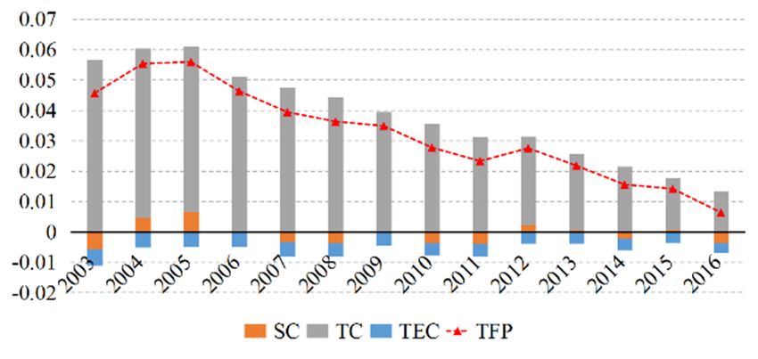
Sustainability 2020, 12, 4981                                                                                              2 of 21

taking account of economic efficiency, social benefits and environmental sustainability [3,4]. Improving
agricultural productivity and promoting sustainable agricultural development is a more pressing
concern for developing countries with higher rates of food insecurity, malnutrition, and rural
poverty [5,6].
     The importance of agricultural sustainable development is particularly high in south Asia and
southeast Asia. Agriculture has long occupied a particularly important position in the economic and
social development of south and southeast Asian countries, which has exclusively contributed to
providing employment, improving food security, and reducing poverty in these two regions [6–8].
Over recent decades, south Asia and southeast Asia have undergone rapid economic growth and
extensive structural changes. Based on the statistics of World Bank data presented in Table 1, the average
GDP growth rate of south Asia and southeast Asia were 5.5% and 6.3% per year, respectively, during
the period 2003–2016. However, the growth rate of agriculture on average was only around 3.2%
for south and southeast Asia during the same period. Southeast Asian countries even experienced
a reduced production in agriculture with an average growth rate of −0.08% in 2016. Furthermore,
the share of agriculture in GDP is shrinking over time, while that of services and manufacture is
increasing. Agriculture’s share of GDP in south and southeast Asian countries reduced from 22% in
2003 to less than 19% in 2016. The slowing growth and declining share of agriculture raises attention to
the importance of promoting sustained agricultural growth in these two regions. Despite the decline
of agriculture’s share in the economy, agricultural employment still accounted for around 47.4% and
38.9% of total employment in major south Asian and southeast Asian countries, respectively, during
the period 2003–2016. Comparatively, the share of agricultural employment in south Asia is higher
than in southeast Asia.

                      Table 1. Agriculture development in south and southeast Asian countries.

                    GDP Growth          Agriculture Growth         Agriculture, Value         Agriculture Employment
       Year
                    (Annual %)              (Annual %)             Added (% of GDP)           (% of Total Employment)
                                                          South Asia
      2003                6.27                   4.01                       22.06                         52.56
      2016                6.77                   2.51                       16.90                         42.82
      mean                5.54                   3.24                       18.76                         47.35
                                                        Southeast Asia
      2003                7.43                   7.48                       21.68                         46.05
      2016                6.50                  −0.08                       15.23                         32.21
      mean                6.30                   3.20                       18.89                         38.86
      Note: The statistics are based on data from eight south Asian countries (Afghanistan, Bangladesh, Bhutan, India, Iran,
      Nepal, Pakistan and Sri Lanka) and seven southeast Asian countries (Cambodia, Indonesia, Malaysia, Myanmar,
      the Philippines, Thailand, Vietnam) from the World Bank database.

     It is obvious that the sustainable development of agriculture in south and southeast Asia
faces plenty of challenges. First, there is increasing domestic and foreign demand for food due to
continued economic growth, rising population and increasing involvement in international trade [4,9].
Second, there are frequent losses of agricultural labor force and arable land because of extensive
structural changes and urbanization [10]. In addition, climate change and natural disasters have
led to land degradation and reductions in water availability, which impose pressure on agricultural
production [11,12]. Furthermore, food insecurity, malnutrition and rural poverty remain as issues to be
addressed in south and southeast Asian countries [13]. Therefore, how to guarantee adequate food
supply and sustainable agriculture production under these aforementioned challenges is an arduous
task for the agricultural sectors in south and southeast Asia.
     Faced with growing food demand with limited agricultural land and labor resources, enhancing
agricultural productivity becomes the most indispensable and effective solution to increase agricultural
production, ensure food security, reduce poverty and malnutrition, and maintain environmental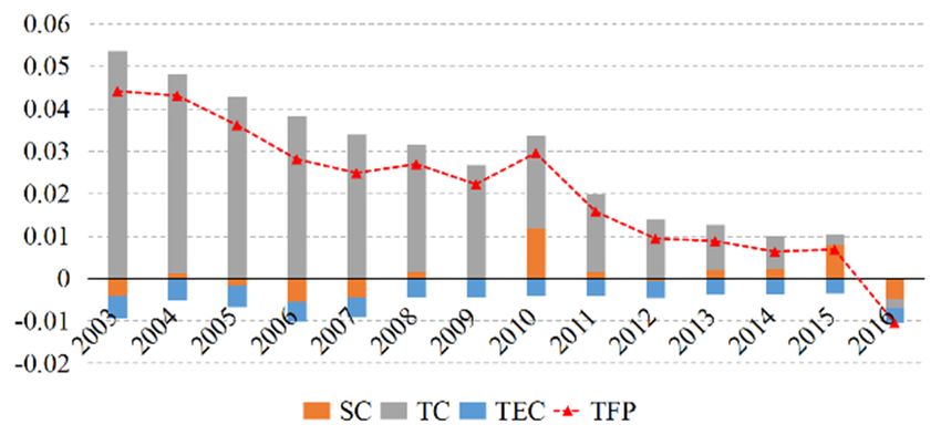
Sustainability 2020, 12, 4981                                                                      3 of 21

sustainability in these two regions. Agricultural total factor productivity (TFP) is viewed as a
representative indicator to assess sustainable development of the agricultural sector [6]. Although
the concept of sustainability incorporates biophysical, economic and social dimensions, we focus
on the economic and social dimensions of sustainability because time series data on biophysical
aspects of agriculture for our study regions are not available, a point also raised by Anik et al. [6]
when analyzing agricultural productivity growth and sustainability in four South Asian countries.
As an appropriate measure to assess sustainability, agricultural TFP should have a non-negative
trend in a sustainable production system. This is because agricultural TFP ensures production by
taking advantage of technological progress, promoting the effective utilization of resources, and saving
the economic and environmental costs of agricultural production [14]. Therefore, a clear map of
agricultural productivity growth and the identification of its influencing factors are crucial to assess
the sustainability of agricultural production in south and southeast Asian countries for the future.
     Given the above background, the objectives of this study are twofold. The first is to estimate the
annual growth of agricultural TFP for eight south Asian countries (Afghanistan, Bangladesh, Bhutan,
India, Iran, Nepal, Pakistan and Sri Lanka) and seven southeast Asian countries (Cambodia, Indonesia,
Malaysia, Myanmar, the Philippines, Thailand, Vietnam) using country-level data covering the period
2002–2016. Cross-country comparisons for south and southeast Asia can be useful as countries in
the two regions have many similarities in terms of geography, production practices and policies,
and economic and social environments [6,15]. The selected 15 countries are all traditional agricultural
countries in south and southeast Asia, and thus are typical and representative examples to study
and compare agricultural development between regions and countries. Based on stochastic frontier
analysis (SFA), the growth of agricultural TFP will be decomposed into three sources: technical change,
technical efficiency change, and scale change, thereby enabling a clear understanding of the different
changing patterns of agricultural TFP in different countries and over time. The second objective is to
identify the key socio-economic factors influencing the growth of agricultural productivity in south
and southeast Asia, which could shed new light on explaining agricultural growth from the viewpoints
of social and economic indicators, thereby providing relevant policy recommendations to promote
agricultural productivity growth under the goal of sustainable development.

2. Literature Review
     Total factor productivity (TFP) is a broad measure of agricultural productivity performance.
TFP explains how efficiently inputs are utilized in production under the influence of technology, policy,
trade, and other various factors [16]. TFP can be decomposed into the different shares explained by
each component of productivity growth, which helps to identify the different sources of productivity
growth, such as technical change, technical efficiency change, and scale efficiency change [17,18].
     There have been numerous studies focusing on the agricultural productivity of developing
countries, and many of them paid attention to the region or countries of sub-Saharan Africa [18–20]
and China [21–23]. Relatively less research has been conducted on agricultural productivity of south
and southeast Asian countries. Sujan et al. [15] analyzed the agricultural productivity of ten south
and southeast Asian countries from 1980 to 2007 and concluded that southeast Asia experienced a
higher growth rate in agricultural production than south Asia. Anik et al. [6] assessed TFP and its
six efficiency components for four south Asian countries, Bangladesh, India, Nepal, and Pakistan,
for the period 1980 to 2013. Their results revealed that the agricultural productivity of these four
countries experienced sustained growth. There have also been some studies focusing on the agricultural
productivity of individual countries, such as Bangladesh [24], India [25–28] and Nepal [29] in south
Asia, and Indonesia [30] and Vietnam [31–33] in southeast Asia.
     Regarding the factors affecting agricultural productivity, empirical studies first suggested that
indicators of economic development, such as income level, urbanization, and industrialization,
were crucial determinants of agricultural TFP growth [25,34–36]. Second, many studies found that
human capital positively contributed to the growth of agricultural productivity [6,36,37]. Third,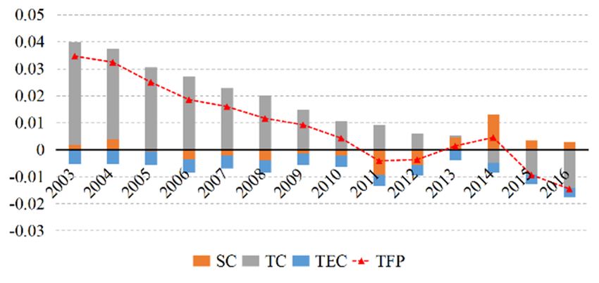
Sustainability 2020, 12, 4981                                                                       4 of 21

agricultural trade affects productivity significantly, although conclusions in this regard have been
ambiguous. Some studies have shown that agriculture trade, both import and export, has positive
influence on agricultural productivity through international spillovers [38,39], while other researchers
have argued that international competition may cause an exodus of human and physical capital from
local firms, leading local agricultural firms to become less productive [40]. In addition, financial
development and assistance to agriculture were also found to be essential to the growth of agricultural
productivity, although conclusions were mixed. Zakaria et al. [36] and Ssozi et al. [41] suggested that
there is a positive relationship between financial development and agricultural productivity, while
Anik et al. [6] found financial capital to have a negative sign as a determinant of agricultural TFP. In
addition, factors such as research, government spending, institutional quality, and climate have also
been identified as key determinants of agricultural productivity.
     As for research methods, stochastic frontier analysis (SFA) and data envelopment analysis (DEA)
were the most used tools in the field of productivity estimation. Compared with traditional index
number approaches, such as Fisher’s (1922) and Törnqvist’s (1936) productivity indices, SFA (parametric
approach) and DEA (non-parametric approach) do not require price information or technical and
behavioral assumptions [17]. A great deal of studies have applied DEA to estimate agricultural
productivity, such as Anik et al. [6], Rezitis [42], and Li et al. [43]. However, some scholars have
argued that DEA-derived TFP always draws inconsistent conclusions, as DEA cannot distinguish
productivity from measurement errors and white noise [22,23]. Moreover, the issues regarding random
or measurement errors are especially prominent for productivity analysis at the macro level [44]. Instead,
SFA allows the separation of inefficiency from random shocks or measurement errors, thus providing a
more accurate estimate of efficiency [18,45]. Given this advantage, SFA has been applied in various
studies to analyze agricultural productivity and its components, such as by Benedetti et al. [46], Adetutu
and Ajayi [18], and Gong [23].
     Existing studies have provided valuable theoretical foundations and empirical findings on
agricultural productivity and its influencing factors. However, despite the important roles of south
and southeast Asia in the world economy and agriculture, not much insight has been gained into the
agricultural productivity and sustainability of south and southeast Asian countries. Also, research
has seldom investigated the influencing factors on agricultural productivity in south and southeast
Asia. The contributions of this study to the related literature are as follows. First, this study
compensates for the lack of literature on agricultural productivity and its influencing factors for south
and southeast Asian countries at regional levels. By comparing differences in agricultural productivity
growth and its components across regions and countries, a more comprehensive understanding of
the agricultural development of south and southeast Asia is gained. Second, most studies of the
agricultural productivity of south Asia and southeast Asia were carried out by nonparametric approach.
We adopt the stochastic production frontier model to estimate agricultural productivity, which can
separate measurement errors from estimated efficiency scores, thereby providing new evidence to
support the related literature under a parametric analytical framework.

3. Methodology and Data

3.1. Decomposition of Total Factor Productivity
     Following Kumbhakar and Lovell [17], stochastic frontier analysis (SFA) was employed for the
estimation and decomposition of TFP changes. A single-output stochastic production frontier model
can be expressed as
                                   yit = f (Xit , t, β) exp(−uit ),                            (1)

where yit represents the value of agricultural production of country i in time t, and Xit donates the set
of input variables. A time trend variable t is included to capture technology progress arising from
exogenous sources. The error component uit measures technical inefficiency, which is a non-negative
random variable and assumed to have a half-normal distribution in our study.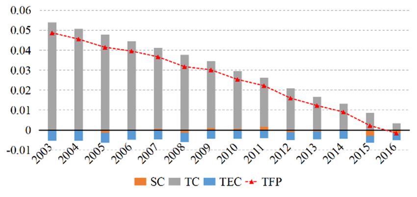
Sustainability 2020, 12, 4981                                                                           5 of 21

      Taking the logarithm for both sides of Equation (1), we get

                                                    lnyit = ln f (Xit , t, β) − uit .                      (2)

      The technical efficiency of production for country i in time t is expressed as

                                                        TEit = exp(−uit ).                                 (3)

      The productivity change is defined as
                                                .         .     .         .
                                                                               XJ
                                               TFP = y − X = y −                             S jx j,       (4)
                                                                                       j=1

                                                                      wjxj
where the dot represents the rate of change, S j = E is the expenditure share of inputs x j , w j donates
                                                               P
price of inputs x j , and total expenditure is expressed as E = j w j x j .
     According to Equation (2), the rate of change of production y is derived by

                                                                      J
                           .  ∂lny   ∂ln f (X, t, β) X ∂ln f (X, t, β) ∂lnx j dx j ∂u
                           y=      =                +                 ·      ·    −    .                   (5)
                               ∂t           ∂t             ∂lnx j       ∂x j dt     ∂t
                                                                    j=1

Equation (5) can be written as

                                           .        ∂ln f (X, t, β) X .         ∂u
                                           y=                      +   ε jx j −    ,                       (6)
                                                           ∂t        j          ∂t

     The symbol ε j represents the elasticities of output with respect to each input: the total elasticities
of output sum to ε = j ε j , which can also be regarded as the return to scale index. Substituting
                       P

Equation (6) into Equation (4), we get

                                .   ∂ln f (X, t, β)           X      .
                                                                           X               .    ∂u
                          TFP =                     + (ε − 1)     ξ jx j +     (ξ j − S j )x j − ,         (7)
                                           ∂t                   j            j                  ∂t

where ξ j = ε j /ε. However, the information on input prices is not available. Thus, it can be simply
assumed that ξ j = S j for all j. Then, the decomposition of TFP change (TFPC) can be simplified to

                                                ∂ln f (X, t, β)           X      .     ∂u
                                    TFPC =                      + (ε − 1)     ξ jx j −    .                (8)
                                                       ∂t                   j          ∂t

      In Equation (8), technical change (TC) is represented as

                                                                    ∂ln f (X, t, β)
                                                        TC =                        .                      (9)
                                                                           ∂t
      Positive values of TC imply technical progress. The scale change (SC) component is calculated by
                                                                                         .
                                                                              X
                                                      SC = (ε − 1)                    ξ jx j.            (10)
                                                                                  j

      If ε − 1 > 0, it implies increasing returns to scale, and the expansion of inputs use will contribute to
the growth of productivity. Diseconomies of scale occur when ε − 1 < 0, and the increase of inputs use
will result in the deterioration of productivity. The rate of technical efficiency change (TEC) is given by

                                                                              ∂u
                                                              TEC = −            .                       (11)
                                                                              ∂t
      A positive value of TEC represents a reduction in inefficiency.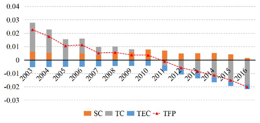
Sustainability 2020, 12, 4981                                                                                           6 of 21

      Now, the changes in TFP have been decomposed into three components, technical change, technical
efficiency change and scale change, which can be written as

                                                  TFPC = TC + SC + TEC.                                                  (12)

     Scale change represents changes in the scale of production, which can be understood as movements
towards or away from the optimal scale. Technical change can be understood as improvements in best
practices, while technical efficiency change measures the extent to which actual production practices
move closer to best practices.
     The translog production frontier model with four inputs is expressed as

                                          4                                4 P
                                                                             4
                           lnyit = β0 +         β j lnx jit + βt t +   1
                                                                                      β jk lnx jit lnxkit + 12 βtt t2
                                          P                                P
                                                                       2
                                          j=1                              j=1 k =1
                                                 4                                                                       (13)
                                                       βit lnx jit t + αr Dr + vit − uit .
                                                 P
                                           +
                                                 j=1

where yit is the agricultural production value added of country i and time t, x jit is the j-th agricultural
input factor, and t is the time trend variable. Further, we added a regional dummy variable Dr to
capture unobserved regional heterogeneities.
    Following Battese and Coelli [47], the inefficiency term uit is defined as

                                                    uit = ui exp(−η[t − T ]),                                            (14)

where ui represents the technical inefficiency effect for the i-th production unit which is assumed to
be half-normally distributed in this study, and η represents the rate of change in technical efficiency.
Positive values of η indicate improvements in technical efficiency over time [48].

3.2. Dynamic Panel Data Models
     The first-difference generalized method of moments (FD-GMM) estimator and system generalized
method of moments (SYS-GMM) estimators in dynamic panel data models were applied to explain the
determinants of agricultural productivity growth in south and southeast Asian countries. The basic
form of a dynamic panel data model is given by

                                      yit = γyi,t−1 + βXit + αi + εit , γ < 1                                            (15)

where yit indicates changes of agricultural TFP for country i (i = 1, 2, . . . , N) at time t (t =
2, 3, . . . , T), Xit = (x1it , x2it , . . . , xkit )0 is a vector of k explanatory variables that explains TFP changes,
and γ and β are parameters to be estimated. The fixed effects decompositions of the error term are
represented by (αi + εit ), and αi is the so-called individual-specific error which captures unobserved
effects that are different across countries but fixed across time. Taking the first differences of Equation (15)
to eliminate individual effects, we get the first difference equation:

                                            ∆yit = γ∆yi,t−1 + β∆Xit + ∆εit .                                             (16)

     In Equation (16), ∆yi,t−1 is endogenous because it is correlated with ∆εit . To solve this problem
of endogeneity, Anderson and Bond [49] proposed the FD-GMM estimator, which is also called
the Arellano–Bond estimator. The FD-GMM estimator applies all possible lags of yi,t−1 and Xit to
construct an instrument matrix under the moment conditions E( yi,t−2 ∆εit ) = 0 and E(xi,t−1 ∆εit ) = 0.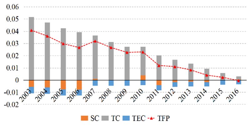
Sustainability 2020, 12, 4981 7 of 21
The instrument matrix Wid for estimating the difference of Equation (16) under the two moment
conditions can be expressed by
yi1 0 0 ··· 0 ··· 0 X0i2
yi1 yi2 ··· ··· X0i3
0 0 0
d
Wi = , (17)
.. .. .. .. .. ..
. . . ··· . ··· . .
0 0 0 ··· yi1 ··· yi,T−2 X0i,T−1
where ( yi1 , yi2 , . . . , yi,t−2 ) indicate the GMM-type instruments at time t which contribute to multiple
columns of the instrument matrix. In addition, the first differences of all exogenous variables Xit are
applied as standard instruments. Using the instrument matrix Wid , Equation (16) can be estimated
under the GMM framework. Detailed explanations and the proof process of the FD-GMM estimator
can be referred to in Anderson and Bond [49] and Carstensen and Toubal [50].
The SYS-GMM estimator, proposed by Blundell and Bond [51], is a system estimation of both
the level equation (Equation (15)) and the first difference equation (Equation (16)). The SYS-GMM
estimator uses additional moment conditions E(∆yi,t−1 εit ) = 0 and E(∆xi,t−1 εit ) = 0 to improve the
small sample performance of the FD-GMM estimator. The corresponding instrument matrix for the
level equation is given by
∆yi2 ∆x0i2
0 ··· 0
∆yi3 ··· ∆x0i3
0 0
l
Wi = . . (18)
.. .. .. ..
. ··· . .
0 0 ··· ∆yi,T−1 ∆x0i,T−1
Then, the system instrument matrix can be obtained by
Wid
" #
0
Wil = . (19)
0 Wil
The SYS-GMM estimator provides an alternative to the FD-GMM estimator; for detailed
explanations see Blundell and Bond [51] and Carstensen and Toubal [50].
3.3. Data Descriptions
To estimate the production frontier function described above, data on the net agriculture production
value added were used to represent agricultural output. Following Fuglie [52] and Adetutu and
Ajayi [18], we considered four agricultural inputs to estimate the production frontier, which were
land, labor, capital, and fertilizer. Agricultural land referred to land used for cultivation of crops and
animal husbandry. Agricultural labor was represented by total population working in agriculture.
Capital input was proxied by the net capital stocks, which reflect physical investment flows after
deducting the portion of assets that are depreciated. The net capital stocks of agriculture were deflated
and transformed from the values of current local currencies to constant 2005 international dollars.
After land, labor, and capital, material inputs also need to be taken into account when estimating
agricultural productivity and efficiency. Fertilizer is a commonly used material input during the
agricultural production process, which is measured as the sum of nutrient nitrogen (N), phosphate
(P2 O5 ), and potash (K2 O). Considering data availability, fertilizer use was selected as a representation
of material inputs into the estimation of agricultural productivity. We did not use seed because reliable
information on seed for all countries under consideration is limited. Furthermore, seed tends to be
used in fixed proportion relative to the amount of land cultivated, and therefore creates a problem of
collinearity with the land variable under the parametric estimation method.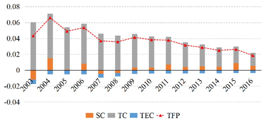
Sustainability 2020, 12, 4981                                                                                     8 of 21

     Based on the existing literature and data availability, we considered six variables to explain the
changes in agricultural TFP. These variables were income level [34,36], human capital [6,36,37],
agricultural export and import [38–40], level of urbanization [25,35] and development flow to
agriculture [6,36,41]. Income level was represented by GDP per capita, which was converted into 2005
international dollars. Mean years of schooling was used as a proxy for human capital. Agricultural
export (import) was calculated as the ratio of agricultural export (import) value to GDP. The urbanization
level was proxied by the ratio of urban population to total population. Furthermore, we applied
the shares of development flow to agriculture to investigate the influence of agricultural aid from
all donors on changes of TFP. The data on development flow to agriculture (DFA) provided by the
Food and Agriculture Organization of the United Nations (FAO) is composed of official development
assistance (ODA) flows, other official flows (OOFs), and private grant/flows from donor countries.
     We collected country-specific data on agricultural output and input variables from eight south
Asian countries and seven southeast Asian countries covering a 15-year period of 2002–2016 to estimate
changes of agricultural TFP. Therefore, a total of 225 observations were included in our data set.
Subsequent changes in the agricultural TFP of these 15 countries from 2003 to 2016 were obtained by
employing SFA. Afterwards, variables explaining TFP changes collected from our sample countries
during 2003–2016 were used to identify the determinants of agricultural productivity growth using
dynamic panel data models. The descriptions and data sources of all variables are presented in Table 2,
and descriptive statistics of the variables are displayed in Table 3. The logarithm forms of agricultural
production, the four agricultural inputs, and GDP per capita were applied in the estimations.

                                 Table 2. Descriptions of variables with data sources.

           Variables                               Description of Variables and Source of Data
                                           Agricultural Output and Inputs
                                 Net agriculture production value added in millions of 2004–2006 international
  Agricultural production        dollars collected from the Food and Agriculture Organization of the United
                                 Nations (FAO).
                                 Total population working in agriculture calculated based on agriculture
             Labor               employment data from the World Bank (WB) database (modeled International
                                 Labour Organization (ILO) estimated).
              Land               Agriculture land area (1000 hectare) from FAO.
                                 Net capital stocks of agriculture in millions of 2005 international dollars
            Capital
                                 from FAO.
                                 Total value of nutrient nitrogen (N), nutrient phosphate (P2 O5 ) and nutrient
           Fertilizer
                                 potash (K2 O) for agriculture use (tons) from FAO.
      Regional dummy             D = 1 for south Asian countries, 0 otherwise.
                            Determinants of Agricultural Total Factor Productivity Change
        GDP per capita           GDP per capita from WB (converted into 2005 international dollars).
                                 Mean years of schooling from Human Development Data (1990–2018) from
        Human capital
                                 United Nations Development Program.
     Agricultural export         Ratio of agricultural export value to GDP from FAO.
     Agricultural import         Ratio of agricultural import value to GDP from FAO.
         Urbanization            Urban population (% of total population) from WB.
      Development flow           Share of total aid to agriculture to total development flow from FAO.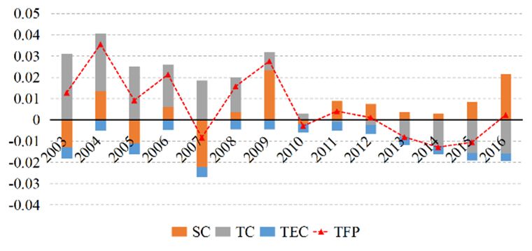
Sustainability 2020, 12, 4981                                                                                        9 of 21

                                         Table 3. Descriptive statistics of variables.

                           Variables                        Obs.       Mean         Std. Dev.   Min       Max
                                       Agricultural Outputs and Inputs (2002–2016)
       Agriculture production (millions$2005 ppp)            225       31,168        52,198     160.8    261,429
                  Land (1000 hectare)                        225       29,554         43,749    519.0    180,560
              Capital (millions$2005 ppp)                    225      107,341        228,271    160.0   1,219,638
                     Fertilizer (tons)                       225      28,01,040     5,775,778   1010    28,373,686
                     Determinants of Agricultural Total Factor Productivity Change (2003–2016)
              GDP per capita ($2005 ppp)                     210       4469.2        3894.9     744.8    17,429.6
                 Human capital (years)                       210       6.151         2.545      2.300     11.000
                 Agriculture export (%)                      210        3.217         2.703     0.171     11.985
                 Agriculture import (%)                      210       7.510          4.163     1.718     20.088
                   Urbanization (%)                          210        36.41         16.30     14.54     74.84
           Development flow to agriculture (%)               210        5.828         5.406     0.180      41.17

4. Results and Discussion

4.1. Drivers of Agricultural Production: Stochastic Production Frontier Model Results
      The estimated results of the production function by SFA are presented in Table 4. The estimated
coefficients represent elasticities of agricultural output with respect to inputs. The coefficient of Labor
is 0.1799, implying that a 1% increase in agriculture labor on average will increase agricultural output
by 0.18%. Similarly, the elasticities of agricultural output with respect to Land (Fertilizer) are 0.60%
(0.06%), indicating that a 1% increase in agricultural land (fertilizer) will increase agricultural output
by 0.60% (0.06%). It can be concluded that the agricultural outputs of south and southeast Asian
countries in our sample were most sensitive to changes in agricultural land, followed by changes
in agricultural labor and fertilizer. However, the estimated coefficient of Capital is positive but not
statistically significant, indicating that capital formulation in agriculture has not made obvious and
significant contributions to the growth of agricultural output. Moreover, the coefficient of the time
trend variable (Time) is positive and significant, while the coefficient of Time squared is significantly
negative. This result indicates that the changes in agricultural productivity in our sample countries
experienced a nonlinear trend, which increased at the beginning and started to decrease after reaching
a certain point. Moreover, the coefficient of the regional dummy variable is negative and significant at
1% level, implying that south Asian countries experienced a lower growth rate of agriculture output
than southeast Asian countries.

                                  Table 4. Estimation results of production function.

                                          Variables                Coef.          Std. Error
                                             Labour            0.1799 ***          0.0267
                                              Land             0.6049 ***          0.0357
                                            Capital              0.0223            0.0441
                                           Fertilizer           0.0583 *           0.0299
                                        Labour squared         0.4343 ***          0.0314
                                         Land squared         −0.8832 ***          0.0611
                                        Capital squared       −0.5349 ***          0.1015
                                       Fertilizer squared       −0.0102            0.0222
                                         Labour*Land            −0.0463            0.0349
                                        Labour*Capital          −0.0113            0.0424
                                       Labour*Fertilizer      −0.0521 **           0.0203
                                         Land*Capital          0.5283 ***          0.0564
                                        Land*Fertilizer         −0.0168            0.0253
                                       Capital*Fertilizer        0.0313            0.0475
Sustainability 2020, 12, 4981                                                                                          10 of 21

                                                        Table 4. Cont.

                                         Variables                Coef.          Std. Error
                                          Time                 0.0457 ***           0.0067
                                      Time squared            −0.0043 ***           0.0008
                                      Labour*Time              0.0119 ***           0.0026
                                       Land*Time              −0.0196 ***           0.0040
                                      Capital*Time             0.0213 ***           0.0054
                                     Fertilizer*Time            −0.0018             0.0032
                                     Region dummy             −0.2596 ***           0.0262
                                        Constant               0.3125 ***           0.0310
                                            σ2u
                                          trend                −0.0655 *            0.0388
                                          _cons               −3.0465 ***           0.3021
                                            σ2v
                                          _cons               −6.5340 ***           0.5796
                                     Log-likelihood             197.45
      Note: the variables of inputs and outputs have been normalized by subtracting local mean value; significance at the
      0.01, 0.05, and 0.10 levels is indicated by ***, **, and *, respectively.

4.2. Agricultural Total Factor Productivity Growth and Its Decomposition
     The agricultural TFP growth was decomposed into scale change (SC), technical change
(TC), and technical efficiency change (TEC) according to the method described in Section 3.1.
The annual changes in TFP (TFPC) and its components are presented in Table 5. Positive values
of TFPC indicate improvements of TFP, whereas the negative values represent the deterioration of
productivity performance.

      Table 5. Annual changes in total factor productivity (TFPC) in agriculture and its components: scale
      change (SC), technical change (TC), and technical efficiency change (TEC).

                                  Year         TFPC          SC             TC         TEC
                                  2003         0.0244      −0.0024        0.0321      −0.0053
                                  2004        −0.1263      −0.1496        0.0284      −0.0052
                                  2005         0.0047      −0.0158        0.0256      −0.0050
                                  2006        −0.0191      −0.0364        0.0221      −0.0048
                                  2007         0.0257      0.0119          0.0184     −0.0047
                                  2008        −0.0070      −0.0172        0.0148      −0.0045
                                  2009         0.0436      0.0372          0.0108     −0.0044
                                  2010        −0.0043      −0.0071        0.0071      −0.0042
                                  2011         0.0200      0.0208          0.0033     −0.0041
                                  2012        −0.0298      −0.0264        0.0005      −0.0040
                                  2013        −0.0172      −0.0104        −0.0029     −0.0038
                                  2014        −0.0485      −0.0385        −0.0062     −0.0037
                                  2015         0.0011      0.0147         −0.0099     −0.0036
                                  2016        −0.0175      −0.0004        −0.0135     −0.0035
                                  Mean        −0.0107      −0.0292        0.0093      −0.0043
      Note: the mean values of changes in agricultural TFP and its components are presented; the year 2003 refers to the
      changes between 2002 to 2003.

     We observed that agricultural TFP in south and southeast Asian countries on average decreased
by 1.07% from 2003 to 2016. The changes in agricultural TFP were not stable over time. In some years
we witnessed improvements in productivity. For other years, however, the agricultural TFP decreased
on average. The average scale change was −2.92% which was the major source of the deterioration
of agricultural productivity. In most years, the values of SC were always negative, indicating that
agricultural TFP in general has not benefited from economies of scale. On the contrary, technical change
on average improved by 0.93%, which implies that technical progress contributed to the improvement
Sustainability 2020, 12, 4981 11 of 21
of agricultural productivity in south and southeast Asia. The value of TC remained positive from 2003
to 2012 with a decreasing trend, while it turned negative after 2012. This result reflects a slowdown of
technical progress in the agricultural sectors of the sample countries. On the other hand, the technical
efficiency change, with an average annual rate of −0.43%, also resulted in a decrease of TFP. The values
of TEC remained negative every year, implying that there was a persistent increase in inefficiency.
To summarize, technical progress is the only source that contributed to the growth of agricultural
productivity, whereas declining scale and technical efficiency changes both resulted in the decline of
agriculture TFP in south and southeast Asian countries.
Next, we disentangled the estimations of agricultural TFP and its components at region and
country levels, to understand the region and country-specific characteristics of agricultural productivity
growth. Table 6 displays the changes in agricultural TFP and its components for the 15 south and
southeast Asian countries. At the regional level, we found a negative average growth rate (−2.96%) in
agricultural TFP for south Asia, indicating an unsustainable route of agricultural development. On the
contrary, the agricultural TFP of southeast Asian countries on average increased by 1.08% during
the sample period. The decrease in agricultural TFP in south Asian countries was largely due to the
negative scale change (−3.06%). On the contrary, technical change, with an average growth rate of
0.54%, was the major source of agricultural productivity growth. As for southeast Asia, scale change
and technical change, with average growth rates of 0.13% and 1.38% respectively, both contributed to
agricultural TFP growth. Like south Asia, technical progress was also the major source driving the
improvement of agricultural TFP in southeast Asian countries.
Table 6. Changes in total factor productivity (TFPC) and its components by country.
Countries TFPC SC TC Countries TFPC SC TC
South Asia Southeast Asia
Afghanistan −0.1059 −0.0679 −0.0336 Cambodia −0.0267 0.0033 −0.0256
Bangladesh 0.0196 −0.0022 0.0262 Indonesia 0.0380 0.0034 0.0390
Bhutan −0.0486 0.0121 −0.0564 Malaysia 0.0075 −0.0026 0.0144
India 0.0691 0.0091 0.0643 Myanmar 0.0013 0.0048 0.0009
Iran −0.2088 −0.1988 −0.0056 Philippines 0.0257 −0.0003 0.0303
Nepal 0.0062 0.0037 0.0068 Thailand 0.0090 0.0001 0.0133
Pakistan 0.0321 −0.0008 0.0373 Vietnam 0.0208 0.0005 0.0247
Sri Lanka −0.0002 0.0004 0.0038
Mean −0.0296 −0.0306 0.0054 Mean 0.0108 0.0013 0.0138
Note: the value of technology efficiency change (TEC) is −0.0043, which is a constant for all countries; SC: scale
change; TC: technical change.
Regarding specific countries in south Asia, Bangladesh, India, Pakistan, and Nepal in general
all experienced improvements in agricultural productivity during the sample period. This result is
supported by Anik et al. [6] who also found a positive growth rate for agricultural TFP for Bangladesh,
India, and Pakistan during the period 2001–2013. The estimated growth rate of agricultural TFP for
India (6.91%) was the highest among south Asian countries, followed by Pakistan (3.21%), Bangladesh
(1.96%), and Nepal (0.62%). Technical change contributed most to the growth of agricultural TFP for all
four countries. India plays a leading role in the economy of south Asian countries and is a major food
producer and consumer. The high growth rate of agricultural TFP in India can not only contribute to
maintaining the self-sufficiency of Indian agricultural production, but also help to meet the additional
food demand of its neighboring countries.
On the contrary, we found negative growth rates of agricultural TFP in Afghanistan (−10.59%),
Bhutan (−4.86%), and Iran (−20.88%). The sharp decline of scale efficiency was the major cause for
the deterioration of agricultural productivity in both Afghanistan and Iran. In the past decades,
the agriculture of Afghanistan and Iran has faced many challenges due to prolonged conflicts and
natural disasters. The shortage of water, lack of irrigation land, and devastating damage to ruralSustainability 2020, 12, 4981 12 of 21
infrastructure have resulted in the loss of scale efficiency and largely held back agricultural productivity.
Unlike Afghanistan and Iran, the decline of agricultural TFP in Bhutan resulted from the obvious
reduction in technical efficiency (−5.64%). Minten and Dukpa [53] also mentioned that the low
level of technology led to low agricultural productivity in Bhutan. Therefore, promoting technical
innovation and progress should be the primary task for Bhutan to achieve the sustainable development
of agriculture.
As for southeast Asia, except for Cambodia, the other six southeast Asian countries all experienced
improvements in agricultural productivity. The growth rate of agricultural TFP for Indonesia (3.80%)
was the highest, followed by the Philippines (2.57%), Vietnam (2.08%), Thailand (0.90%), and Malaysia
(0.75%). Like south Asia, technical progress made the dominant contribution to improving the
agricultural TFP in these five countries. The growth rate of agricultural TFP in Myanmar was only
0.13%. Unlike the other five countries, the scale change (0.48%) largely contributed to agricultural
TFP growth, while technical efficiency change was the major factor holding back the agricultural
productivity of Myanmar.
Cambodia is the only country in southeast Asia that experienced an average drop of −2.67% in
agricultural productivity during the sample period. The retrogression of technology in Cambodia was
the main reason for the deterioration of agricultural productivity, a somewhat similar situation to that
of Bhutan. In comparison with south Asian countries, southeast Asian countries overall showed a
more sustained and stable growth in agricultural productivity, which is in accordance with the findings
by Sujan et al. [15] who concluded that the average agricultural production growth was higher in
southeast Asia than south Asia.
To explain the changing characteristics of agricultural TFP for each country more intuitively,
the annual TFP changes and their three components for south Asian and southeast Asian countries are
plotted in Figure 1; Figure 2, respectively. As shown in Figure 1, the agricultural TFP exhibited similar
growth patterns in Bangladesh, India, and Pakistan. Each country observed a positive growth rate of
agricultural TFP every year, with considerable contributions due to technical progress. The continued
TFP growth indicated that the development of agricultural productivity in the three countries was
relatively steady and robust. Technical change was rising continuously throughout the sample period,
indicating continuous improvements in the technological innovation of the agricultural sectors in
the three countries. Thus, we can conclude that the agricultural developments of Bangladesh, India,
and Pakistan were at the forefront among the south Asian countries. However, it should be noted
that the growth speed of agricultural TFP in the three countries was decreasing along with technical
progress. As a result, how to provide enough growth momentum for technology innovation may have
been the major challenge that the agriculture sectors in these three countries faced.
Unlike Bangladesh, India, and Pakistan, changes of agricultural TFP in Afghanistan and Iran
fluctuated over time and were dominated by scale efficiency decline. Moreover, the growth patterns
of agricultural TFP in Nepal and Sri Lanka were also not stable but showed some similarities.
Both countries experienced technical progress at the beginning; however, the backward technology and
reduced technical efficiency dragged down agricultural productivity from 2012. Moreover, Bhutan was
the only south Asian country where agricultural TFP deteriorated every year. The technical change and
technical efficiency change both declined each year, which had a negative impact on the agricultural
productivity of Bhutan.sample period, indicating continuous improvements in the technological innovation of the
agricultural sectors in the three countries. Thus, we can conclude that the agricultural developments
of Bangladesh, India, and Pakistan were at the forefront among the south Asian countries. However,
it should be noted that the growth speed of agricultural TFP in the three countries was decreasing
along with technical progress. As a result, how to provide enough growth momentum for technology
Sustainability 2020, 12, 4981 13 of 21
innovation may have been the major challenge that the agriculture sectors in these three countries
faced.
(a) Afghanistan (b) Bangladesh
(c) Bhutan (d) India
(e) Iran (f) Nepal
(g) Pakistan (h) Sri Lanka
Figure 1. Changes in agricultural total factor productivity (TFP) and its components in south Asia
(SC: scale change; TC: technical change; TEC: technical efficiency change).
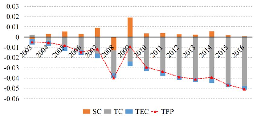
There were also several different growth patterns of agricultural productivity in southeast Asia
(see Figure 2). First, the growth of agricultural TFP tended to slow down in Indonesia, Myanmar,
the Philippines, Thailand, and Vietnam. India exhibited the best practices regarding agricultural
production in the southeast Asian region; the continuous technical progress was a great help to its
sustainable agricultural development. The slowdown trends of agricultural productivity growth in
Myanmar, the Philippines, Thailand, and Vietnam were more obvious over time. The agricultural TFP
of Myanmar and Thailand started to decline from 2011, while the growth rate of agricultural TFP in the
Philippines and Vietnam also turned negative in 2016. The persistent slowdown of technical progress
was the common factor driving the deterioration of agricultural TFP in these countries.production in the southeast Asian region; the continuous technical progress was a great help to its
sustainable agricultural development. The slowdown trends of agricultural productivity growth in
Myanmar, the Philippines, Thailand, and Vietnam were more obvious over time. The agricultural
TFP of Myanmar and Thailand started to decline from 2011, while the growth rate of agricultural TFP
in the Philippines and Vietnam also turned negative in 2016. The persistent slowdown of technical
Sustainability 2020, 12, 4981 14 of 21
progress was the common factor driving the deterioration of agricultural TFP in these countries.
(b) Indonesia
(a) Cambodia
(c) Malaysia (d) Myanmar
Sustainability 2020, 12, x FOR PEER REVIEW
(e) Philippines (f) Thailand
(g) Vietnam
Figure 2. Changes of agricultural
Figuretotal factor productivity
2. Changes (TFP)
of agricultural and
total its components
factor productivityin(TFP)
Southeast Asia
and its components in Southeast As
(SC: Scale Change; TC: Technical change; TEC: Technical efficiency change).
(SC: Scale Change; TC: Technical change; TEC: Technical efficiency change).
Unlike the other southeast Asian countries, the agricultural TFP changes in Malaysia fluctuated,
Unlike the other southeast Asian countries, the agricultural TFP changes in Malaysia fluc
and this was mainly affected by scale change. A possible reason is that agriculture in Malaysia is still
and this was mainly affected by scale change. A possible reason is that agriculture in Malaysia
dominated by smallholders with an ageing farmer population, thereby causing diseconomies of scale
dominated by smallholders with an ageing farmer population, thereby causing diseconomies o
in agricultural production [54]. Consolidating efficient and professional management of small farms is
in agricultural production [54]. Consolidating efficient and professional management of smal
crucial for Malaysia to promote scale benefits in agricultural production. Like Bhutan, Cambodia was
is crucial for Malaysia to promote scale benefits in agricultural production. Like Bhutan, Cam
the only southeast Asian country that experienced a continuous deterioration of agricultural TFP due
was the only southeast Asian country that experienced a continuous deterioration of agricultu
due to technical regression and efficiency decline. The technical regression of agricult
Cambodia worsened during the sample period.
4.3. Factors Explaining Agricultural TFP Changes
In this subsection, we applied the FD-GMM estimator to dynamic data models to expl
determinants of agricultural TFP changes in south and southeast Asian countries. The estSustainability 2020, 12, 4981 15 of 21
to technical regression and efficiency decline. The technical regression of agriculture in Cambodia
worsened during the sample period.
4.3. Factors Explaining Agricultural TFP Changes
In this subsection, we applied the FD-GMM estimator to dynamic data models to explain the
determinants of agricultural TFP changes in south and southeast Asian countries. The estimated results
of the SYS-GMM estimator are also provided as a robustness check. The presence of endogeneity
could result in inconsistent estimated results, but the problem can be addressed by instrumental
variables [55,56]. In dynamic panel data models, the FD-GMM and SYS-GMM estimators can deal
with the problem of endogeneity by using instrumental variables [50,57]. The estimated parameters
of the dynamic FD-GMM estimator and the results of model diagnostics are presented in Table 7.
The statistics from Sargan’s test rejected the null hypothesis that the over-identifying restrictions were
valid, suggesting that the instrument variables as a group were exogenous, and that the choice of
instruments was reasonable in our model. Meanwhile, the results of Arellano–Bond tests for zero
autocorrelation in the first-difference disturbances showed that the disturbances were not serially
correlated. The null hypothesis of the Wald test is that “the coefficients on the explanatory variables
are jointly zero”, which was strongly rejected, implying that the inclusion of explanatory variables
was reasonable.
Table 7. Dynamic first-difference generalized method of moments (FD-GMM) and system generalized
method of moments (SYS-GMM) estimators for the determinants of TFP changes.
Models FD-GMM SYS-GMM
Variables Coef. Std.Error Coef. Std.Error
Lagged change in TFP −0.0598 0.0397 −0.0753 ** 0.0298
GDP per capita −0.1879 *** 0.0265 −0.1690 *** 0.0315
Human capital 0.0386 * 0.0216 0.0626 *** 0.0190
Agricultural export −0.0002 0.0060 0.0113 0.0073
Agricultural import −0.0137 *** 0.0012 −0.0104 *** 0.0019
Urbanization 0.0246 *** 0.0059 0.0012 0.0041
Development flow 0.0037 *** 0.0002 0.0038 *** 0.0002
Time dummy 1(=1 from 2003 to 2007) 0.0387 *** 0.0083 −0.0281 ** 0.0108
Time dummy 2(=1 from 2008 to 2012) 0.0480 *** 0.0085 0.0106 0.0064 *
Constant 0.4183 * 0.2523 0.9592 *** 0.1947
Model Diagnostics
Wald test (chi2 ) 50,406.38 8087.92
Wald test (p value) 0.0000 0.0000
Sargan’s test (chi2 ) 12.204 10.612
Sargan’s test (p value) 1.0000 1.0000
Arellano–Bond test for AR (1)
(z-statistic) −1.0835 −1.1180
(p value) 0.2786 0.2636
Arellano–Bond test for AR (2)
(z-statistic) 0.9859 0.9846
(p value) 0.3242 0.3248
Note: Significance at the 0.01, 0.05, and 0.10 levels are indicated by ***, **, *, respectively; AR (1): first-order
autocorrelation; AR (2): second-order autocorrelation.
The level of economic development, measured by GDP per capita, was significant and negatively
correlated with agricultural TFP change, indicating that higher income levels were associated with
a slower growth in agricultural TFP. Many south and southeast Asian countries were in a period of
economic transformation with increasing shares of industry and services. The share of agriculture
in total GDP was declining, but employment in agriculture still accounted for a large proportion
of employment in these countries. This phenomenon implies that the agricultural productivitySustainability 2020, 12, 4981 16 of 21
of these countries was not keeping pace with economic development. Consequently, south and
southeast Asian countries experienced slower agricultural productivity growth despite continuous
economic development.
Human capital positively contributed to the growth of agricultural productivity. Human capital
can directly increase a worker’s productivity, thus contributing to improvements in agricultural TFP.
This result is consistent with the findings by Lanzona [58], Anik et al. [6], and Zakaria et al. [36],
who also focused on the agricultural productivity of south Asian or southeast Asian countries and
concluded that agricultural productivity increased with an increase in human capital. However, some
studies found a negative role of human capital on agricultural productivity. For example, Rahman
and Salim [59] mentioned that human capital significantly contributed to technical progress but had a
negative impact on technical efficiency, scale efficiency, and TFP growth in Bangladesh.
Regarding agricultural trade, we found a negative relationship between agricultural import and
TFP changes. In theory, developing countries can learn advanced technologies and management
experience through importing goods and services from developed countries, which is the so-called
demonstration effect, thereby contributing to the improvement of productivity. Nevertheless, there
may also be a loss of human and physical capital for local firms due to international competition,
leading to the backwardness of agricultural productivity [39]. The negative value of agricultural
import in this study indicated that domestic agricultural products faced fierce competition from
imported products but without the obvious benefits of the demonstration effect. On the other hand,
agricultural export can help to achieve economies of scale by expanding markets overseas. Exporters
also can improve their technological innovation capacities through experience from international
competition [31]. However, our result shows no significant effect of agricultural export on agricultural
TFP, though it may exist theoretically.
Urbanization was positively associated with changes in agricultural productivity. With limited
land resources, urbanization contributes to the transformation of the labor force from the countryside to
urban areas, thereby promoting the rational reallocation of agricultural labor input. In addition, farmers
in suburban areas can take advantage of the proximity to urban centers to reduce costs. Therefore,
urbanization is helpful to improve efficiency and accelerate productivity growth. The positive impact
of urbanization on agricultural productivity is also evident in work by Kumar et al. [25] and Oueslati
and Wu [60]. However, it has been argued that urbanization may have adverse effects on agricultural
productivity, because urban land expansion will lead to cropland loss, which has become a major
concern in terms of food production and supply [61]. The key issue is whether the growing demand
for food and more convenient access to the market due to urbanization can maintain the sustainable
development of agriculture given the decline of agricultural land [62].
The development flow to agriculture positively contributed to the growth in agricultural TFP.
Therefore, the development assistance to agricultural sectors was effective in improving the agricultural
productivity of south and southeast Asian countries. Ssozi et al. [41] also found a positive relationship
between development assistance and agricultural productivity. The two time dummy variables were
both significant and positive, which indicated that the earlier periods experienced a higher growth
rate of agricultural productivity. This result reveals that the growth rate of agricultural TFP in south
and southeast Asian countries declined significantly. However, the lagged changes in TFP showed no
significant association with TFP changes in current periods.
The signs and significance level for the coefficients of most explanatory variables in the SYS-GMM
model were consistent with the results in the FD-GMM model. Concretely speaking, human capital and
development flow to agriculture were confirmed to have a significant positive influence on changes in
agricultural TFP, whereas GDP per capita and agricultural import still showed significant negative
signs in the SYS-GMM model. The results of a robustness test further verified the credibility of our
findings for factors affecting changes in agricultural productivity in south and southeast Asia.Sustainability 2020, 12, 4981 17 of 21
5. Conclusions and Policy Recommendations
This study examined the agricultural productivity growth of 15 south and southeast Asian
countries from 2002 to 2016 using a stochastic frontier model in order to assess the sustainability of
their agricultural sectors. Through the decomposition of TFP, we identified scale change, technical
change, and technical efficiency change as the components of agricultural productivity growth.
Subsequently, the influencing factors on agricultural productivity change in south and southeast Asia
were investigated using dynamic panel data models. The main conclusions of this study can be drawn
as follows:
South and southeast Asian countries overall witnessed declined agricultural productivity during
the period 2002–2016, reflecting the unsustainable development route of their agricultural sectors.
Technical progress made major contributions to agricultural productivity growth. As mentioned by
Huang and Chien [63], the lack of environmental and social sustainability is a principal problem
existing in the agriculture sector, while innovation is the key to solving this problem. On the contrary,
scale and technical efficiency change both resulted in a decline in agriculture TFP. At the regional level,
south Asia experienced agricultural productivity deterioration overall, although there was obvious
technical progress in some south Asian countries during the sample period, such as India, Pakistan,
and Bangladesh. On the contrary, there were improvements in agricultural productivity in southeast
Asia over time, owing to the progress of technology. In comparison with south Asian countries,
southeast Asian countries have achieved more stable and sustained growth in agriculture productivity.
Agricultural productivity in the countries of south and southeast Asia faced different growth
patterns. In the first place, many south and southeast Asian countries, including Bangladesh,
India, Pakistan, and Nepal in south Asia, as well as Indonesia, the Philippines, Vietnam, Thailand,
and Malaysia in southeast Asia, on average experienced improvements in agricultural productivity
mainly powered by technical progress. Next, Myanmar also witnessed a slight increase in agricultural
productivity; however, the improvement was largely the result of gains from scale efficiency. On the
contrary, Afghanistan and Iran experienced an obvious productivity deterioration because of the loss
of scale efficiency, while weakened technology was the major cause for productivity decline in Bhutan
and Cambodia.
The changes in agricultural TFP showed several dynamic characteristics. First, the growth speed of
agricultural TFP slowed down together with technical progress in many countries, such as Bangladesh,
India, Nepal, Pakistan, and Sri Lanka in south Asia, as well as Indonesia, Myanmar, the Philippines,
Thailand, and Vietnam in southeast Asia. Among them, the agricultural TFP of Nepal, Sri Lanka,
Myanmar, the Philippines, Thailand, and Vietnam gradually changed from an increase to a decline.
Second, agricultural productivity in Bhutan and Cambodia kept falling every year because of the
continued backwardness of technology. Third, changes in agricultural TFP in Afghanistan and Iran had
obvious fluctuations over time due to unstable scale changes. Therefore, diseconomies of scale may be
one of the major challenges for the sustained development of agriculture in Afghanistan and Iran.
Furthermore, our results indicate that human capital, urbanization, and development flow to
agriculture are crucial factors that contributed significantly to the agricultural productivity growth of
south and southeast Asian countries. On the contrary, income level and agricultural import were found
to be negatively associated with agricultural productivity growth. In addition, we found no positive
relationship between the lagged level and current level of TFP changes, implying that agriculture
development in south Asia and southeast Asia overall has not been directed toward a sustainable path.
Based on the above conclusions, the following policy recommendations are proposed to promote
productivity growth and the sustainable development of agriculture sectors in south and southeast
Asia. First, south and southeast Asian countries should focus on technological innovation to increase
productivity. Second, major frontier countries in the two regions, such as India and Indonesia,
should take the lead on regional agricultural development and focus on enhancing cooperation with
neighboring countries in terms of agricultural science and frontier technologies. Third, countries
such as Afghanistan and Iran, which might face challenges from diseconomies of scale, should attachYou can also read