A monthly tidal envelope classification for semidiurnal regimes in terms of the relative proportions of the S2, N2, and M2 constituents - OS
←
→
Page content transcription
If your browser does not render page correctly, please read the page content below
Ocean Sci., 16, 965–977, 2020
https://doi.org/10.5194/os-16-965-2020
© Author(s) 2020. This work is distributed under
the Creative Commons Attribution 4.0 License.

A monthly tidal envelope classification for semidiurnal regimes in
terms of the relative proportions of the S2, N2, and M2 constituents
Do-Seong Byun1 and Deirdre E. Hart2
1 Ocean    Research Division, Korea Hydrographic and Oceanographic Agency, Busan 49111, Republic of Korea
2 School   of Earth and Environment, University of Canterbury, Christchurch 8140, Aotearoa/New Zealand

Correspondence: Deirdre E. Hart (deirdre.hart@canterbury.ac.nz)

Received: 28 November 2019 – Discussion started: 11 December 2019
Revised: 2 June 2020 – Accepted: 16 June 2020 – Published: 18 August 2020

Abstract. Daily tidal water level variations are a key con-      1   Introduction
trol on shore ecology, on access to marine environments via
ports, jetties, and wharves, on drainage links between the       Successful human–coast interactions in the world’s low-
ocean and coastal hydrosystems such as lagoons and estu-         lying areas are predicated upon understanding the temporal
aries, and on the duration and frequency of opportunities to     and spatial variability of sea levels (Nicholls et al., 2007;
access the intertidal zone for recreation and food harvesting    Woodworth et al., 2019). This is particularly the case in is-
purposes. Further, high perigean spring tides interact with      land nations like New Zealand (NZ), where over 70 % of the
extreme weather events to produce significant coastal inun-      population resides in coastal settlements (Stephens, 2015).
dations in low-lying coastal settlements such as on deltas.      An understanding of tidal water level variations is fundamen-
Thus an understanding of daily through monthly tidal enve-       tal for resilient inundation management and coastal develop-
lope characteristics is fundamental for resilient coastal man-   ment practices in such places, as well as for accurately re-
agement and development practices. For decades, scientists       solving non-tidal signals of global interest such as in studies
have described and compared daily tidal forms around the         of sea level change (Cartwright, 1999; Masselink et al., 2014;
world’s coasts based on the four main tidal amplitudes. Our      Olson, 2012; Pugh, 1996; Stammer et al., 2014).
paper builds on this “daily” method by adjusting the con-           In terms of daily cycles, tidal form factors or form num-
stituent analysis to distinguish between the different monthly   bers (F ) based on the amplitudes of the four main tidal con-
types of tidal envelopes occurring in the semidiurnal coastal    stituents (K1 , O1 , M2 , S2 ) have been successfully used to
waters around New Zealand. Analyses of tidal records from        classify tidal observations from the world’s coasts into four
27 stations are used alongside data from the FES2014 tide        types of tidal regimes for nearly a century (Fig. 1a). Origi-
model in order to find the key characteristics and constituent   nally developed by van der Stok (1897) and based on three
ratios of tides that can be used to classify monthly tidal en-   regime types, with a fourth type added by Courtier (1938),
velopes. The resulting monthly tidal envelope classification     this simple and useful daily form factor comprises a ratio be-
approach described (E) is simple, complementary to the suc-      tween diurnal and semidiurnal tide amplitudes via the equa-
cessful and much used daily tidal form factor (F ), and of use   tion
for coastal flooding and maritime operation management and            K1 + O1
planning applications in areas with semidiurnal regimes.         F=           .                                             (1)
                                                                      M2 + S2
                                                                 The results classify tides into those which roughly experi-
                                                                 ence one high and one low tide per day (diurnal regimes),
                                                                 two approximately equivalent high and low tides per day
                                                                 (semidiurnal regimes), or two unequal high and low tides
                                                                 per day (mixed semidiurnal-dominant or mixed diurnal-
                                                                 dominant regimes) (e.g. Defant, 1958).

Published by Copernicus Publications on behalf of the European Geosciences Union.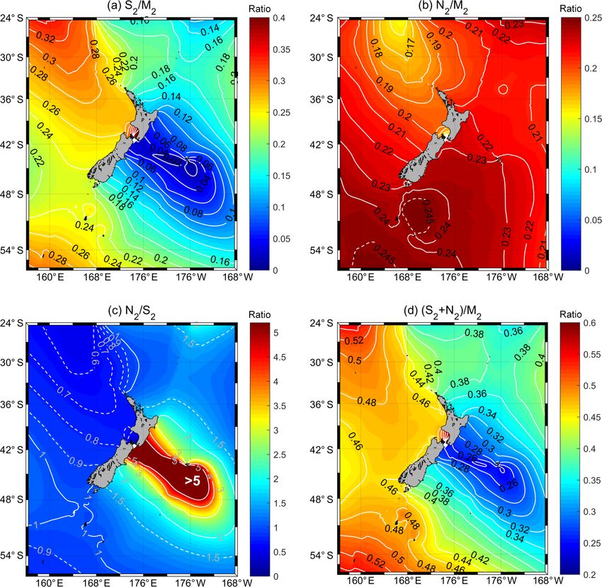
966 D.-S. Byun and D. E. Hart: A monthly tidal envelope classification for semidiurnal regimes
ber (1 or 2) and form (equal or unequal tidal ranges) of tidal
cycles within a lunar day (i.e. 24 h and 48 min) at a partic-
ular site. In contrast, the term “tidal envelope” describes a
smooth curve outlining the extremes (maxima and minima)
of the oscillating daily tidal cycles occurring at a particular
site through a specified time period. The envelope time pe-
riod of interest in this paper is monthly.
Tidal envelopes at monthly scales depend on tidal regime.
In general, semidiurnal tidal regimes often feature two
spring–neap tidal cycles per synodic (lunar) month. These
two spring–neap tidal cycles are usually of unequal mag-
nitude due to the effect of the moon’s perigee and apogee,
which cycle over the period of the anomalistic month. In
contrast, diurnal tidal regimes exhibit two pseudo-spring–
neap tides per sidereal month. For semidiurnal regions where
the N2 constituent contributes significantly to tidal ranges,
tidal envelope classification should consider relationships be-
tween the M2 , S2 , and N2 amplitudes. The waters around
NZ represent one such region; here the daily tidal form is
consistently semidiurnal, but large differences occur between
sites within this region in terms of their typical tidal enve-
lope types over fortnightly to monthly timescales. More than
80 years after the development of the ever-useful daily tidal
form factors, attention to the regional distinctions between
different tidal envelope types within the semidiurnal category
forms the motivation for this paper. In this first explicit at-
tempt to classify monthly tidal envelope types, we examined
the waters around NZ, a strong semidiurnal regime with rel-
atively weak diurnal tides (daily form factor F < 0.15) and
little variation in the importance of the S2 and N2 ampli-
tude ratios. The result is an approach for classifying monthly
tidal envelope types that is transferable to any semidiurnal
regime. As well as providing greater understanding of the
tidal regimes of NZ, we hope that our paper opens the door
for new international interest in classifying tidal envelope
variability at multiple timescales, which is work that would
have direct coastal and maritime management applications
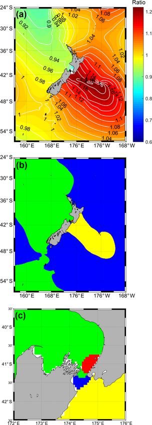
Figure 1. (a) Global distribution of daily form factor (F ) values in-
including contributing to explanations of the processes be-
dicating daily tidal regime types (F < 0.25: semidiurnal; F > 0.25
to F < 1.5 mixed semidiurnal dominant; F > 1.5 to F < 3: mixed
hind delta cities’ coastal flooding hazards and their regional
diurnal dominant; and F > 3: diurnal; according to the classifica- spatial variability.
tion of van der Stok, 1897, and Courtier, 1938); (b) the world’s
semidiurnal tidal areas (F < 0.25) divided into those where spring–
neap (green) versus perigean–apogean (blue) signals are the main 2 Methodology
influence on the monthly tidal envelope; and (c) semidiurnal tidal
regimes (in red) in which the S2 /M2 constituent amplitude ratio is 2.1 Study area
< 0.04 and the spring–neap tidal signals are very weak as compared
to perigean–apogean signals; derived from FES2014 tidal harmonic New Zealand (Fig. 2) is a long (1600 km), narrow (≤ 400 km)
constants. country situated in the south-western Pacific Ocean and
straddling the boundary between the Indo-Australian and Pa-
cific plates. Its three main islands, the North Island, the South
Albeit not part of their original design, some interpreta- Island, and Stewart Island/Rakiura, span a latitudinal range
tion of the tidal envelope types observed at fortnightly and from about 34◦ to 47◦ S. The tidal regimes in the surround-
monthly timescales has accompanied the use of daily tidal ing coastal waters are semidiurnal with variable diurnal in-
form classifications (e.g. Pugh, 1996; Pugh and Woodworth, equalities, and they feature micro through macro tidal ranges.
2014). The daily tidal form factor identifies the typical num- Classic spring–neap cycles are present in western areas of
Ocean Sci., 16, 965–977, 2020 https://doi.org/10.5194/os-16-965-2020
D.-S. Byun and D. E. Hart: A monthly tidal envelope classification for semidiurnal regimes                                         967

                                                                       2.2    Data analysis approach

                                                                       Year-long sea level records were sourced from a total of 27
                                                                       stations spread around NZ (Fig. 2): 18 records of 1 min in-
                                                                       tervals from Land Information New Zealand (LINZ, 2017a)
                                                                       and nine records of 1 h intervals from the National Institute
                                                                       of Water and Atmospheric Research (NIWA, 2017). For both
                                                                       the LINZ and NIWA data, an individual year of good-quality
                                                                       hourly data was selected for analysis per site from amongst
                                                                       the multi-year records. The 27 single-year sea level records
                                                                       were then harmonically analysed using T_Tide (Pawlowicz
                                                                       et al., 2002) with the nodal (satellite) modulation correction
                                                                       option to examine spatial variations in the main tidal con-
                                                                       stituents’ amplitudes, phase lags, and amplitude ratios be-
                                                                       tween regions (see Table A1 for raw results) and to compare
                                                                       them with values obtained from the tidal potential or equi-
                                                                       librium tide. An additional set of tidal constituent amplitudes
                                                                       was obtained from Tables 1 and 3 from Walters et al. (2010),
                                                                       which was derived from 33 records of between 14 and 1900 d
                                                                       in length from around the greater Cook Strait area, where
                                                                       spring–neap tides are the strongest in the country.
                                                                          We then classified the monthly tidal envelope types found
                                                                       around NZ based on the examination of constituent ratios
                                                                       produced from the tidal harmonic analysis results, data from
                                                                       the FES2014 tide model (see Carrère et al., 2016, for a full
                                                                       description of this model), and examination of tidal enve-
Figure 2. Location of New Zealand sea level observation stations       lope plots. Due to the strong semidiurnal tidal regimes in the
investigated in this research. Each site is coloured according to      study area, and in a similar way to the approach of Walters
monthly tidal envelope type. Offshore islands are not shown to scale   et al. (2010), we were able to ignore diurnal (K1 , O1 ) effects
(Raoul and Chatham islands).                                           and simply consider the effects of spring–neap (M2 , S2 ) and
                                                                       perigean–apogean cycles (M2 , N2 ) in our monthly tidal en-
                                                                       velope type characterisation.
NZ, while eastern areas feature distinct perigean–apogean
influences (Byun and Hart, 2015; Heath, 1977, 1985; LINZ,
2017b; Walters et al., 2001).                                          3     Results
   Highly complex tidal propagation patterns occur around
NZ, including a complete semidiurnal tide rotation, with               3.1    Key tidal constituent amplitudes and amplitude
tides generally circulating around the country in an anticlock-               ratios
wise direction. This occurs due to the forcing of M2 and N2
tides by their respective amphidromes, situated north-west             In order to better understand the key constituents responsible
and south-east of the country respectively, producing trapped          for shaping tidal height forms around NZ, we first mapped
Kelvin waves (for a map of the K1 and M2 amphidromes,                  spatial variability in the amplitudes of the M2 , S2 , N2 K1 ,
see Fig. 5.1 in Pugh and Woodworth, 2014). The S2 and K1               and O1 constituents and F (Fig. 3) and in the ratio values of
tides propagate north-east to south-west around NZ. This re-           the semidiurnal constituent amplitudes (Fig. 4). Table 1 sum-
sults in a southward travelling Kelvin wave along the west             marises these data and contrasts them with those from equi-
coast and small S2 and K1 amplitudes along the east coast,             librium theory (values obtained from Defant, 1958), while
with amphidromes occurring south-east of NZ (Walters et al.,           Table A1 catalogues the detailed results.
2001, 2010). Around Cook Strait, the waterway between the                 Tidal amplitude ratio comparisons confirmed that the wa-
two main islands, tides travelling north along the east coast          ters around NZ are dominated by the three astronomical se-
run parallel to tides travelling south along the west coast.           midiurnal tides: M2 , S2 , and N2 (Table 1), the combina-
The pronounced differences between these east–west tidal               tion of which can generate fortnightly spring–neap tides (M2
states, combined with their tidal range differences, together          and S2 ) and monthly perigean–apogean tides (M2 and N2 ).
produce marked differences in amplitude and strong current             Figure 3 shows the relatively minor magnitudes of diurnal
flows through the strait (Heath, 1985; Walters et al., 2001,           constituent amplitudes (O1 , K1 ), and it reveals the stronger
2010).                                                                 west coast amplitudes of the spring–neap-cycle-generating

https://doi.org/10.5194/os-16-965-2020                                                               Ocean Sci., 16, 965–977, 2020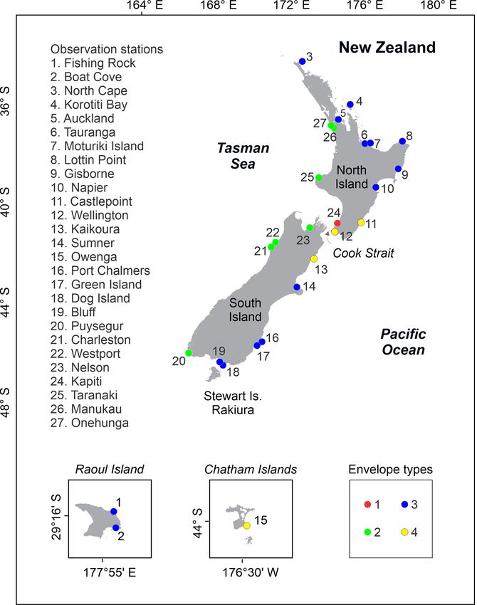
D.-S. Byun and D. E. Hart: A monthly tidal envelope classification for semidiurnal regimes
https://doi.org/10.5194/os-16-965-2020
Table 1. Comparison of tidal constituent amplitudes, amplitude ratios (including daily tidal form factor, F , and monthly tidal envelope factor, E), and ranges between the four distinct
monthly tidal envelope types found in the 27 case study semidiurnal tide regimes of New Zealand and compared to equilibrium theory amplitude ratios. n/a: not applicable.
Envelope type Example sites Amplitude (cm) Amplitude ratio F value range and E value range and
description description
S2 N2 N2 S2 S2 +N2 K1 O1
M2 S2 N2 K1 O1 M2 M2 S2 N2 M2 M2 M2
n/a Equilibrium – – – – – 0.47 0.19 0.41 2.44 0.66 0.58 0.42 0.68 mixed, mainly n/a
theory semidiurnal
1 Kapiti 55 26 9 2 2 0.47 0.16 0.35 2.89 0.64 0.04 0.04 0.05 semidiurnal 0.790 spring–neap
2 Nelson, 78 to 133 19 to 40 17 to 25 2 to 6 1 to 4 0.24 to 0.3 0.18 to 0.22 0.58 to 0.89 1.12 to 1.74 0.45 to 0.48 0.02 to 0.06 0.01 to 0.05 0.04 to 0.07 semidi- 0.902 to 0.979 in-
Manukau, urnal termediate, spring–
Taranaki, neap dominant
Onehunga,
Westport,
Charleston,
Puysegur Point
3 North Cape, 50 to 112 4 to 18 10 to 22 2 to 8 1 to 4 0.06 to 0.2 0.2 to 0.23 1.07 to 3.5 0.29 to 0.94 0.28 to 0.43 0.02 to 0.10 0.01 to 0.06 0.05 to 0.14 semidi- 1.011 to 1.147
Boat Cove and urnal intermediate,
Fishing Rock perigean–apogean
(Raoul Island), dominant
Dog Island,
Auckland,
Bluff, Lottin
Point, Tau-
ranga, Korotiti
Bay, Moturiki,
Green Island,
Port Chalmers,
Sumner, Gis-
borne, Napier
4 Kaikoura, 48 to 65 2 to 3 10 to 14 2 to 4 2 to 4 0.04 to 0.05 0.21 to 0.22 4.67 to 5.50 0.18 to 0.21 0.25 to 0.27 0.04 to 0.06 0.04 to 0.06 0.08 to 0.12 semidi- 1.162 to 1.176
Ocean Sci., 16, 965–977, 2020
Owenga, urnal perigean–apogean
Castlepoint,
Wellington
968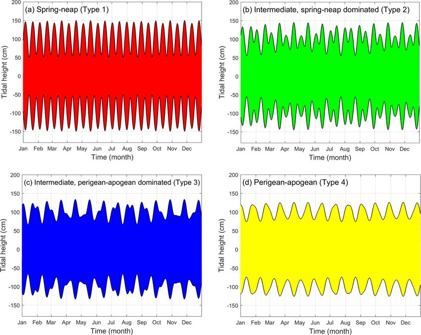
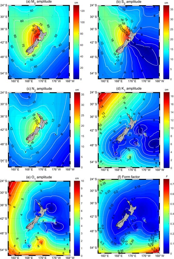
D.-S. Byun and D. E. Hart: A monthly tidal envelope classification for semidiurnal regimes                                                  969

Figure 3. Distribution of amplitudes for the (a) M2 , (b) S2 , (c) N2 , (d) K1 , and (e) O1 tides around NZ and (f) the resultant distribution of
F , daily tidal form factor values, as calculated from the FES2014 tide model on a grid of 1◦ / 16 × 1◦ / 16. Note that the amplitude colour
scales vary between panels (a) and (e).

constituents (M2 and S2 ), the relatively weak S2 amplitudes               smaller values (< 0.3 at 26 out of 27 sites) than that of equi-
overall (half that of equilibrium theory), and the more con-               librium theory (0.47). In contrast, N2 /M2 amplitude ratios
centric pattern around NZ of the perigean–apogean-cycle-                   were found to be more stable around NZ (values ranging
generating N2 amplitude (Fig. 3c).                                         from 0.16 to 0.23) and similar in magnitude to equilibrium
  In terms of the semidiurnal constituent amplitude ratios,                theory (i.e. 0.19). By grouping the constituent amplitude and
Fig. 4 and Table 1 show that S2 /M2 values cover a broad                   amplitude ratio results (Figs. 3–4), we were able to differ-
range around NZ (0.04 to 0.47), with most sites exhibiting                 entiate between four distinct monthly tidal envelope regimes

https://doi.org/10.5194/os-16-965-2020                                                                       Ocean Sci., 16, 965–977, 2020
970                               D.-S. Byun and D. E. Hart: A monthly tidal envelope classification for semidiurnal regimes

Figure 4. Distributions of tidal constituent amplitude ratios around NZ for the following: (a) S2 /M2 , (b) N2 /M2 , (c) N2 /S2 , and (d) S2M
                                                                                                                                            +N2
                                                                                                                                                ,
                                                                                                                                             2
                                                              ◦       ◦
as calculated using the FES2014 tide model on a grid of 1 / 16 × 1 / 16. Note that the amplitude colour scales vary between panels (a)
and (d).

around NZ (Table 1) with types 1 and 4 distinguished as fol-                     phase, as is typical in spring–neap regimes. Type 4
lows.                                                                            regimes occur, for example, around northern Chatham
                                                                                 Rise near Kaikoura and as far north as Castlepoint on
  – Firstly, spring–neap type tidal regimes (Type 1) occur                       the east coast of the North Island.
    where the S2 tide amplitude is large compared to that of
    the N2 (Table 1; Fig. 3). In these areas, there are two                The remaining coastal waters around NZ can be separated
    spring–neap tides per month with similar ranges and                    into two tidal subregions, one with strong spring–neap sig-
    negligible influence of perigean–apogean cycles. Type 1                nals (Type 2) and the other with strong perigean–apogean
    regimes occur in the Kapiti and Cook Strait area (Fig. 2)              signals (Type 3) but both with overall mixed or intermedi-
    where the N2 and M2 amplitudes reduce by 75 % to                       ate monthly tidal envelope types (Table 1). We distinguished
    90 % but the S2 amplitude reduces by only about 30 %                   between these two envelope types via the tides generated
    compared to on the western coasts both north and south                 by variability in the amplitude ratios of S2 /M2 and N2 /M2
    of this central NZ area.                                               (i.e. the spring–neap cycle and perigean–apogean cycle form-
                                                                           ing tides respectively). In brief, the S2 /M2 amplitude ratio
  – In direct contrast, there are perigean–apogean type tidal              varies widely around NZ, with the highest values in the west,
    regimes (Type 4) in areas where the N2 amplitude                       lowest values in the east, and intermediate values to the north
    strongly dominates over the S2 (Table 1; Fig. 3). In                   and south, while variation in the N2 /S2 amplitude ratio ex-
    Type 4 regimes, the M2 and the N2 tides combine to pro-                hibits an opposite pattern (compare Fig. 4a to 4c). By com-
    duce strong signals over monthly timeframes (27.6 d).                  parison, the N2 /M2 amplitude ratios are relatively stable and
    Hence the highest tidal ranges in any given month occur                high except in the relatively small area of the Cook Strait
    in relation to the perigee, when the moon’s orbit brings               to the Kapiti Coast, where this ratio drops and thus spring–
    it close to Earth rather than in line with the moon’s                  neap cycles predominate (see spring–neap Type 1 regimes

Ocean Sci., 16, 965–977, 2020                                                                     https://doi.org/10.5194/os-16-965-2020
D.-S. Byun and D. E. Hart: A monthly tidal envelope classification for semidiurnal regimes 971
above). The variability in these two ratios means that, except with x = N2 /S2 , and
where we find spring–neap or perigean–apogean monthly
N2
tidal envelope types, spring–neap tides do occur but the over- 1+ M2
all monthly envelope shape is fundamentally altered (asym- E= N2
, (2c)
1+ M2
y
metrically) due to the perigean–apogean influence.
with y = S2 /N2 .
– In the first of the intermediate subregions, tides ex-
E takes into account the roles of the S2 and N2 tides in
hibit two dominant but unequal spring–neap cycles per
spring–neap and perigean–apogean cycles while also factor-
month due to subordinate perigean–apogean effects. We
ing in the strong M2 tide influence in both types of cycles.
term this type of monthly tidal envelope an intermedi-
E may be used to classify the monthly tidal envelope types
ate, predominantly spring–neap type regime (Type 2).
of any semidiurnal region (i.e. where F < 0.25) based on the
Here values of the N2 /S2 amplitude ratio are < 1, with
analysis of constituent amplitudes and ratios from local data.
S2 amplitudes being only around 24 % to 30 % of those
The boundaries between our different NZ monthly tidal en-
of the M2 constituent (Figs. 3–4; Table 1). Also in these
velope types were as follows.
areas, values of the S2M+N2
2
amplitude ratio are ≥ 0.45.
Type 2 tides occur, for example, at Westport and Puyse- – E < 0.8 indicates a Type 1 spring–neap regime.
gur.
– E between 0.8 and 1.0 indicates a Type 2 intermedi-
– In the other intermediate subregion, tides exhibit a ate, predominantly spring–neap regime (with the up-
mainly perigean–apogean form with a weaker but no- per bound also corresponding to an amplitude ratio of
ticeable spring–neap signal: we term this envelope N2 /S2 < 1 in semidiurnal regimes).
type as intermediate, predominantly perigean–apogean
(Type 3). Here values of the N2 /S2 amplitude ratio are – E between 1.0 and 1.15 indicates a Type 3 intermedi-
between 1.07 and 3.5, while values of the S2M +N2
am- ate, predominantly perigean–apogean regime (with the
2
plitude ratio are between 0.28 and 0.43 (Figs. 3–4; Ta- lower bound also corresponding to an amplitude ratio of
ble 1). Type 3 tides occur, for example, at Auckland and N2 /S2 > 1 in semidiurnal regimes).
Sumner. – E > 1.15 indicates a Type 4 perigean–apogean regime
(with the lower bound also corresponding to an ampli-
Figure 5 illustrates the four types of monthly tidal envelopes
tude ratio of N2 /S2 > 4 in our NZ regimes).
found around NZ as idealised types, two with stronger
spring–neap signals (types 1 and 2; see Fig. 5a–b) and two Here we explain how we set boundaries between the dif-
with stronger perigean–apogean signals (types 3 and 4; see ferent envelope types around NZ using case study data and
Fig. 5c–d), while Fig. 2 includes a colour coded classifica- as summarised in Fig. 6. Firstly, in any semidiurnal tidal
tion of the observation stations into the four tidal envelope regime (F < 0.25) anywhere in the world where the ampli-
types. tude ratio N2 /S2 < 1, spring–neap cycles will feature clearly
in the tidal height records. Thus, the boundary separating
3.2 A monthly tidal envelope factor (E) for types 1 and 2 from types 3 and 4 occurs at N2 /S2 = 1, when
semidiurnal regimes also E = 1. Type 1 and 2 areas of the NZ coast are char-
acterised by relatively larger S2 amplitudes (19–40 cm) than
The four types of monthly tidal envelopes found around NZ areas with stronger perigean–apogean influences (2–18 cm)
are essentially different combinations of spring–neap and (Table 1). Secondly, tidal regimes with stronger spring–
perigean–apogean signals. Thus, in a similar manner to the neap signals include places where spring–neap cycles oc-
method of Courtier (1938) for calculating daily tidal form cur as consecutive fortnightly cycles of similar magnitudes
factors, a monthly tidal envelope factor (E) may be calculated (Type 1 or spring–neap type regimes) and places where
for semidiurnal tidal regions, including that of NZ, according spring–neap signals dominate but with noticeable variabil-
to the following: ity in the magnitudes of consecutive cycles due to subordi-
nate perigean–apogean influences (Type 2 or intermediate
M 2 + N2
E= , (2a) spring–neap regimes). In NZ, the strongest spring–neap in-
M2 + S2 fluence occurs in the Cook Strait to Kapiti area, where har-
monic analysis revealed an amplitude ratio of N2 /S2 = 0.35
where M2 , N2 , and S2 refer to the constituent amplitudes.
and an E value of 0.79 (Table 1). Examining the shapes
This equation can be further expressed as follows:
of tidal height plots showed that Kapiti had the only com-
S2 pletely spring–neap-dominated tidal envelope amongst the
1+ M x
E= 2
, (2b) case study sites. Hence the boundary between Type 1 versus
S2
1+ M 2
Type 2 was set as E = 0.790 for NZ, which is just greater
https://doi.org/10.5194/os-16-965-2020 Ocean Sci., 16, 965–977, 2020972 D.-S. Byun and D. E. Hart: A monthly tidal envelope classification for semidiurnal regimes Figure 5. Idealised examples of four different monthly tidal envelopes over 1 year, calculated using the amplitude value M2 = 100 cm and the amplitude ratio values of (a) S2 /M2 = 0.46, S2 /N2 = 11.5, and N2 /M2 = 0.04; (b) S2 /M2 = 0.27, S2 /N2 = 1.5, and N2 /M2 = 0.18; (c) S2 /M2 = 0.12, S2 /N2 = 0.54, and N2 /M2 = 0.22; and (d) S2 /M2 = 0.04, S2 /N2 = 0.18, and N2 /M2 = 0.22. Note that the E values of these plots are (a) 0.71, (b) 0.93, (c) 1.09, and (d) 1.17. than that of Kapiti and below the next strongest spring–neap- in detail by Walters et al. (2010); our Fig. 6 includes a re- influenced site, Nelson, where E = 0.902 (Fig. 6). Lastly, analysis of their data using the E ratios. Note that the Cook to set a boundary between perigean–apogean and intermedi- Strait data include four sites in the Type 1 category, as well as ate perigean–apogean-dominant regimes (i.e. Type 3 versus a number of Type 2 and Type 4 sites and one Type 3 site, re- Type 4), we again examined tidal height plots to determine vealing this small strait to be a concentrated area of monthly a boundary value of E = 1.15, which is between the inter- tidal envelope diversity. Extensive areas of Type 3 interme- mediate perigean–apogean-dominated type regime of Napier diate perigean–apogean-dominated regimes are found along (E = 1.147) and the perigean–apogean type regime of Kaik- the north-east and south-east coasts of NZ, while the cen- oura (E = 1.162) (Table A1; Fig. 6). tral eastern coasts show Type 4 perigean–apogean tidal en- In summary, Fig. 7 illustrates the monthly tidal envelope velopes. As shown in Fig. 1c, such regimes are unusual in- values and types in the waters around NZ using E. The west ternationally, occurring also in limited areas of the Cook Is- coast is characterised by Type 2 monthly tidal envelopes with lands, north-east of the Pitcairn Islands, in Canada’s Hudson two unequal spring–neap cycles per month. As mentioned Bay, in Alaska’s Bristol Bay, offshore of the North Carolinian above, Type 1 monthly tidal envelopes, with their defined to Virginian coast in the Unites States of America, on the spring–neap tides, are only found in the western Cook Strait north coast of the Bahamas, and in the Gulf of Ob in Russia. to Kapiti Coast area. The Cook Strait’s tides were explored Ocean Sci., 16, 965–977, 2020 https://doi.org/10.5194/os-16-965-2020
D.-S. Byun and D. E. Hart: A monthly tidal envelope classification for semidiurnal regimes                                                973

Figure 6. Plot of the relationship between the N2 /S2 and S2 /M2
amplitude ratios (y and x axes respectively) and E values (shown
as plot contours), with data points corresponding to New Zealand
waters monthly tidal envelope Type 1 sites (red dots), Type 2 sites
(green dots), Type 3 sites (blue dots), and Type 4 sites (yellow dots)
(all from Table A1), as well as tidal data representative of the greater
Cook Strait area (black stars) from Walters et al. (2010; Tables 1
and 3 therein).

4   Discussion and conclusion

The daily water level variations brought about by the tides
are a key control on shore ecology and on the accessibility
of marine environments via fixed port, jetty, and wharf in-
frastructure. These variations also moderate the functioning
of drainage links between the ocean and coastal hydrosys-
tems and determine the duration and frequency of opportu-
nities to access the intertidal zone for recreation and food
harvesting purposes. Fortnightly and monthly tidal envelope
variations, such as those associated with spring–neap and
perigean–apogean cycles, have similar moderating roles on
human usage of intertidal and shoreline environments, and
additionally these medium term variations in tide levels are
important factors in coastal inundation risk (Menéndez and
Woodworth, 2010; Stephens, 2015; Stephens et al., 2014;
Wood, 1978, 1986). High perigean spring tides, for example,
interact with extreme weather events (including low pres-
sures, strong winds, and extreme rainfall) to produce signifi-
cant coastal inundation in low-lying coastal settlements such
as in the delta city of Christchurch (Hart et al., 2015).
   In a world of rising sea levels and coastal inundation
hazard cascades (Menéndez and Woodworth, 2010), hav-                       Figure 7. (a) Distribution of monthly tidal envelope factor (E) val-
ing common ways of describing different types of tidal en-                 ues and (b) monthly tidal envelope types in the waters around New
velopes is helpful for living safely and productively in coastal           Zealand, including (c) in the Cook Strait area between the two main
                                                                           islands, all calculated using FES2014 data. In (b) and (c), envelope
cities. This paper has employed observations from NZ and
                                                                           Type 1 areas are shown in red, Type 2 in blue, Type 3 in green, and
FES2014 model data to demonstrate a simple approach to
                                                                           Type 4 in yellow. See Fig. 5 for definitions and examples of monthly
classifying different monthly tidal envelope types which is                tidal envelope factor classes and patterns.
applicable to semidiurnal regions anywhere. The result is a

https://doi.org/10.5194/os-16-965-2020                                                                     Ocean Sci., 16, 965–977, 2020
974 D.-S. Byun and D. E. Hart: A monthly tidal envelope classification for semidiurnal regimes
widely applicable monthly tidal envelope factor, E, for clas- Figure 1b illustrates the division of the semidiurnal ar-
sifying semidiurnal regimes based on the amplitudes and am- eas of the world’s oceans into those where spring–neap cy-
plitude ratios of three key constituents: M2 , S2 , and N2 . cles are the main monthly tidal envelope influence versus
At a very basic level, in any semidiurnal tidal regime any- those where the perigean–apogean signal is stronger, while
where in the world where the amplitude ratio of N2 /S2 < Fig. 1c illustrates areas of the world’s oceans where spring–
1, spring–neap cycles will then be clearly visible in tidal neap signals are very weak compared to perigean–apogean
height records either as consecutive fortnightly cycles of sim- influences in the monthly tidal envelope. The predictable
ilar magnitude (Type 1) or as a dominant signal with no- tidal water level fluctuations such as those in our perigean–
ticeable variability in the magnitudes of consecutive fort- apogean monthly envelope classes are an important influence
nightly cycles due to a subordinate perigean–apogean in- on coastal inundation hazards in different locations around
fluence (Type 2). Conversely, in semidiurnal areas of the the world (e.g. Wood, 1978, 1986; Stephens, 2015).
world’s oceans where the amplitude ratio of N2 /S2 > 1, Our simple approach to classifying E, namely monthly
perigean–apogean cycles will then be visible either as sin- tidal envelope types in semidiurnal regions, complements
gularly evident monthly cycles (Type 4) or as a dominant in- the existing, commonly used way of describing daily tidal
fluence with subordinate spring–neap signals (Type 3). De- forms, F , based on the amplitudes of the key diurnal (K1 ,
termining the actual boundaries between monthly tidal en- O1 ) and semidiurnal (M2 , S2 ) constituents. We hope that
velope Type 1 versus Type 2 and Type 3 versus Type 4 at our work inspires other efforts to study tidal height varia-
a local scale involves the analysis of observational records, tions at timescales greater than daily, which could draw re-
taking into account the important influence of the M2 ampli- newed attention to the fundamental role of tidal water levels
tude compared to that of the S2 and N2 amplitudes. in shaping coastal environments, including in hazards such
as coastal flooding.
Ocean Sci., 16, 965–977, 2020 https://doi.org/10.5194/os-16-965-2020D.-S. Byun and D. E. Hart: A monthly tidal envelope classification for semidiurnal regimes 975
Appendix A
Table A1. Monthly tidal envelope types and values of monthly (E) and daily (F ) form factors and data on the amplitude (ai ) and phase lag
(Gi , relative to Greenwich) values of five tidal constituents’ (subscript i) harmonic constants at 27 sea level stations around New Zealand.
Station name (record used) Envelope type E value F value M2 S2 N2 K1 O1
ai Gi ai Gi ai Gi ai Gi ai Gi
(cm) (◦ ) (cm) (◦ ) (cm) (◦ ) (cm) (◦ ) (cm) (◦ )
Kapiti (2011) 1 0.790 0.05 55 280 26 336 9 277 2 195 2 18
Nelson (2015) 2 0.902 0.04 133 276 40 329 23 254 6 187 1 80
Manukau (2011) 2 0.935 0.05 109 297 29 332 20 287 6 17 1 287
Taranaki (2016) 2 0.941 0.05 119 278 33 319 24 257 6 192 2 90
Onehunga (2016) 2 0.945 0.05 131 304 34 359 25 288 6 205 2 118
Westport (2015) 2 0.958 0.04 113 309 29 348 23 287 2 198 3 40
Charleston (2015/2016) 2 0.962 0.05 106 319 27 344 22 304 3 6 3 243
Puysegur Point (2012) 2 0.979 0.07 78 350 19 13 17 335 3 316 4 245
North Cape (2010) 3 1.011 0.11 80 230 15 279 16 209 8 10 2 351
Boat Cove, Raoul Island (2012) 3 1.017 0.14 50 208 9 287 10 176 5 43 3 44
Dog Island (2011) 3 1.028 0.06 91 33 18 57 21 6 2 119 4 60
Auckland (2011) 3 1.039 0.07 112 216 17 275 22 192 7 356 2 324
Bluff (2016) 3 1.040 0.05 84 48 15 75 19 23 2 133 3 71
Fishing Rock, Raoul Island (2011) 3 1.050 0.12 52 206 8 283 11 178 5 35 2 41
Lottin Point (2011) 3 1.063 0.1 70 195 9 262 14 168 6 352 2 328
Tauranga (2011) 3 1.063 0.08 70 211 9 277 14 186 5 0 1 330
Korotiti Bay (2011) 3 1.056 0.08 78 207 11 265 16 181 6 349 1 317
Moturiki (2011) 3 1.060 0.07 73 189 10 265 15 156 5 173 1 136
Green Island (2011) 3 1.084 0.08 73 81 10 91 17 50 3 93 4 44
Port Chalmers (2011) 3 1.093 0.07 77 112 9 112 17 89 3 270 3 247
Sumner (2011) 3 1.133 0.09 84 136 6 151 18 109 5 273 3 245
Gisborne (2010) 3 1.130 0.07 64 176 5 251 14 148 4 336 1 275
Napier (2011) 3 1.147 0.07 64 167 4 240 14 138 3 298 2 221
Kaikoura (2011) 4 1.162 0.12 65 146 3 171 14 117 4 275 4 233
Owenga, Chatham Islands (2011) 4 1.160 0.08 48 149 2 224 10 119 2 246 2 179
Castlepoint (2011) 4 1.167 0.09 63 159 3 225 14 129 3 280 3 219
Wellington (2011) 4 1.176 0.1 49 148 2 352 11 116 2 268 3 219
Overall range 1–4 0.79–1.176 0.04–0.14 48–133 – 2–40 – 9–25 – 2–8 – 1–4 –
https://doi.org/10.5194/os-16-965-2020 Ocean Sci., 16, 965–977, 2020976 D.-S. Byun and D. E. Hart: A monthly tidal envelope classification for semidiurnal regimes
Data availability. The tidal data used in this paper are avail- Courtier, A.: Marées. Service Hydrographique de la Ma-
able from LINZ (2017a, https://www.linz.govt.nz/sea/tides/ rine, Paris, available at: https://journals.lib.unb.ca/index.php/ihr/
introduction-tides/tides-around-new-zealand, last access: article/download/27428/1882520184 (last access: 28 Novem-
28 November 2019), LINZ (2017b, https://www.linz.govt. ber 2019), 1938.
nz/sea/tides/introduction-tides/tides-around-new-zealand, Defant, A.: Ebb and flow: the tides of earth, air, and water, Univer-
last access: 28 November 2019), NIWA (2017, https: sity of Michigan Press, Ann Arbor, 1958.
//www.niwa.co.nz/our-services/online-services/sea-levels (last Hart, D. E., Byun, D.-S., Giovinazzi, S., Hughes, M. W., and
access: 28 November 2019), and Walters et al. (2010). Gomez, C.: Relative Sea Level Changes on a Seismically Ac-
Details of the FES2014 tide model database are found via tive Urban Coast: Observations from Laboratory Christchurch,
https://www.aviso.altimetry.fr/en/data/products/auxiliary-products/ Auckland, New Zealand, Proceedings of the Australasian Coasts
global-tide-fes.html (last access: 28 November 2019) and in and Ports Conference 2015, 15–18 September 2015, 6 pp., 2015.
Carrère et al. (2016). Appendix A contains the data produced from Heath, R. A.: Phase distribution of tidal constituents around New
the analysis of these primary resources in this paper. Zealand, New Zeal. J. Mar. Fresh., 11, 383–392, 1977.
Heath, R. A.: A review of the physical oceanography of the seas
around New Zealand – 1982, New Zeal. J. Mar. Fresh., 19, 79–
Author contributions. Both authors conceived of the idea behind 124, 1985.
this paper. DEH produced the initial draft. DSB analysed the tidal LINZ (Land Information New Zealand): Sea level data downloads,
data and wrote the results sections. Both authors worked on and available at: http://www.linz.govt.nz/sea/tides/sea-level-data/
finalised the full paper. sea-level-data-downloads (last access: 28 November 2019),
2017a.
LINZ (Land Information New Zealand): Tides around New
Competing interests. The authors declare that they have no conflict Zealand, available at: https://www.linz.govt.nz/sea/tides/
of interest. introduction-tides/tides-around-new-zealand (last access:
28 November 2019), 2017b.
Masselink, G., Hughes, M., and Knight, J.: Introduction to Coastal
Processes and Geomorphology, 2nd edn., Routeldge, 432 pp.,
Special issue statement. This article is part of the special
2014.
issue “Developments in the science and history of tides
Menéndez, M. and Woodworth, P. L.: Changes in extreme high wa-
(OS/ACP/HGSS/NPG/SE inter-journal SI)”. It is not associ-
ter levels based on a quasi-global tide-gauge data set, J. Geophys.
ated with a conference.
Res., 115, C10011, https://doi.org/10.1029/2009JC005997,
2010.
Nicholls, R. J., Wong, P. P., Burkett, V. R., Codignotto, J., Hay, J.,
Acknowledgements. We are grateful to Land Information New McLean, R., Ragoonaden, S., Woodroffe, C. D., Abuodha, P. A.
Zealand (LINZ) and the National Institute of Water and Atmo- O., Arblaster, J., and Brown, B.: Coastal systems and low-lying
spheric Research (NIWA) for supplying the tidal data used in this re- areas, in: Climate change 2007: impacts, adaptation and vulner-
search. We thank the University of Canterbury Erskine Programme ability, edited by: Parry, M. L., Canziani, O. F., Palutikof, J. P.,
for supporting Do-Seong Byun during his time in New Zealand, van der Linden, P. J., and Hanson, C. E., Contribution of Work-
John Thyne for supplying the Fig. 2 outline map, and Derek Gor- ing Group II to the fourth assessment report of the Intergovern-
ing for interesting discussions regarding tidal data sources. We also mental Panel on Climate Change, Cambridge University Press,
thank Glen Rowe, Phillip Woodworth, and an anonymous reviewer Cambridge, UK, 315–356, 2007.
for comments that helped us improve this paper. NIWA (National Institute of Water and Atmospheric Research): Sea
level gauge records (hourly interval), available at: https://www.
niwa.co.nz/our-services/online-services/sea-levels (last access:
Review statement. This paper was edited by Mattias Green and re- 28 November 2019), 2017.
viewed by Philip Woodworth and one anonymous referee. Olson, D.-W.: Perigean spring tides and apogean neap tides in his-
tory, American Astronomical Society Meeting Abstracts, 219,
115.03, 2012.
Pawlowicz, R., Beardsley, B., and Lentz, S.: Classical tidal
References harmonic analysis including error estimates in MAT-
LAB using T_TIDE, Comput. Geosci., 28, 929–937,
Byun, D.-S. and Hart, D. E.: Predicting tidal heights for new loca- https://doi.org/10.1016/S0098-3004(02)00013-4, 2002.
tions using 25h of in situ sea level observations plus reference Pugh, D. T.: Tides, surges and mean sea-level (reprinted with cor-
site records: A complete tidal species modulation with tidal con- rections), John Wiley & Sons Ltd, Chichester, UK, 486 pp., 1996.
stant corrections, J. Atmos. Ocean. Tech., 32, 350–371, 2015. Pugh, D. T. and Woodworth, P. L.: Sea-level science: Understand-
Carrère L., Lyard, F., Cancet, M., Guillot, A., and Picot, N.: FES ing tides, surges, tsunamis and mean sea-level changes, Cam-
2014, a new tidal model – validation results and perspectives for bridge University Press, Cambridge, ISBN 9781107028197, 408
improvements, Presentation to ESA Living Planet Conference, pp., 2014.
Prague, 2016. Stammer, D., Ray, R. D., Andersen, O. B., Arbic, B. K., Bosch,
Cartwright, D. E.: Tides: A scientific history, Cambridge University W., Carrère, L., Cheng, Y., Chinn, D. S., Dushaw, B. D., Eg-
Press, Cambridge, 1999.
Ocean Sci., 16, 965–977, 2020 https://doi.org/10.5194/os-16-965-2020D.-S. Byun and D. E. Hart: A monthly tidal envelope classification for semidiurnal regimes 977 bert, G. D., and Erofeeva, S. Y.: Accuracy assessment of global Walters, R. A., Gillibrand, P. A., Bell, R. G., and Lane, E. M.: barotropic ocean tide models, Rev. Geophys., 52, 243–282, A study of tides and currents in Cook Strait, New Zealand, https://doi.org/10.1002/2014RG000450, 2014. Ocean Dynam., 60, 1559–1580, https://doi.org/10.1007/s10236- Stephens, S.: The effect of sea level rise on the frequency of extreme 010-0353-8, 2010. sea levels in New Zealand, NIWA Client Report No. HAM2015- Wood, F. J.: The strategic role of perigean spring tides in nautical 090, prepared for the Parliamentary Commissioner for the Envi- history and North American coastal flooding, 1635–1976, De- ronment PCE15201, Hamilton, 52 pp., 2015. partment of Commerce, University of Michigan Library, 1978. Stephens, S. A., Bell, R. G., Ramsay, D., and Goodhue, N.: High- Wood, F. J.: Tidal dynamics: Coastal flooding and cycles of gravi- water alerts from coinciding high astronomical tide and high tational force, M.A., USA, D. Reidel Publishing Co., Hingham, mean sea level anomaly in the Pacific islands region, J. Atmos. 1986. Ocean. Tech., 31, 2829–2843, 2014. Woodworth, P. L., Melet, A., Marcos, M., Ray, R. D., Wöppelmann, van der Stok, J. P.: Wind and water, currents, tides and tidal streams G., Sasak, I. Y. N., Cirano, M., Hibbert, A., Huthnance, J. M., in the East Indian Archipelago, Batavia, 1897. Monserrat, S., and Merrifield, M. A.: Forcing factors affecting Walters, R. A., Goring, D. G., and Bell, R. G.: Ocean tides around sea level changes at the coast, Surv. Geophys., 40, 1351–1397, New Zealand, New Zeal. J. Mar. Fresh., 35, 567–579, 2001. 2019. https://doi.org/10.5194/os-16-965-2020 Ocean Sci., 16, 965–977, 2020
You can also read