CNN: Single-label to Multi-label
←
→
Page content transcription
If your browser does not render page correctly, please read the page content below

JOURNAL OF LATEX CLASS FILES, VOL. 6, NO. 1, JANUARY 2014                                                                                    1

                                                           CNN: Single-label to Multi-label
                                       Yunchao Wei, Wei Xia, Junshi Huang, Bingbing Ni, Jian Dong, Yao Zhao, Senior Member, IEEE
                                                                 Shuicheng Yan, Senior Member, IEEE

                                         Abstract—Convolutional Neural Network (CNN) has demonstrated promising performance in single-label image classification
                                         tasks. However, how CNN best copes with multi-label images still remains an open problem, mainly due to the complex underlying
                                         object layouts and insufficient multi-label training images. In this work, we propose a flexible deep CNN infrastructure, called
                                         Hypotheses-CNN-Pooling (HCP), where an arbitrary number of object segment hypotheses are taken as the inputs, then a
                                         shared CNN is connected with each hypothesis, and finally the CNN output results from different hypotheses are aggregated with
                                         max pooling to produce the ultimate multi-label predictions. Some unique characteristics of this flexible deep CNN infrastructure
                                         include: 1) no ground-truth bounding box information is required for training; 2) the whole HCP infrastructure is robust to possibly
arXiv:1406.5726v3 [cs.CV] 9 Jul 2014

                                         noisy and/or redundant hypotheses; 3) no explicit hypothesis label is required; 4) the shared CNN may be well pre-trained with a
                                         large-scale single-label image dataset, e.g. ImageNet; and 5) it may naturally output multi-label prediction results. Experimental
                                         results on Pascal VOC2007 and VOC2012 multi-label image datasets well demonstrate the superiority of the proposed HCP
                                         infrastructure over other state-of-the-arts. In particular, the mAP reaches 84.2% by HCP only and 90.3% after the fusion with
                                         our complementary result in [47] based on hand-crafted features on the VOC2012 dataset, which significantly outperforms the
                                         state-of-the-arts with a large margin of more than 7%.

                                         Index Terms—Deep Learning, CNN, Multi-label Classification

                                                                                                               F

                                   1    I NTRODUCTION                                                              real-world images are with more than one objects
                                                                                                                   of different categories. Many methods [37], [6], [12]
                                   S   INGLE-label image classification, which aims to
                                       assign a label from a predefined set to an image,
                                   has been extensively studied during the past few
                                                                                                                   have been proposed to address this more challenging
                                                                                                                   problem. The success of CNN on single-label image
                                   years [14], [18], [10]. For image representation and                            classification also sheds some light on the multi-
                                   classification, conventional approaches utilize care-                           label image classification problem. However, the CNN
                                   fully designed hand-crafted features, e.g., SIFT [32],                          model cannot be trivially extended to cope with the
                                   along with the bag-of-words coding scheme, followed                             multi-label image classification problem in an inter-
                                   by the feature pooling [25], [44], [37] and classic                             pretable manner, mainly due to the following reasons.
                                   classifiers, such as Support Vector Machine (SVM) [4]                           Firstly, the implicit assumption that foreground ob-
                                   and random forests [2]. Recently, in contrast to the                            jects are roughly aligned, which is usually true for
                                   hand-crafted features, learnt image features with deep                          single-label images, does not always hold for multi-
                                   network structures have shown their great potential                             label images. Such alignment facilitates the design of
                                   in various vision recognition tasks [26], [21], [24],                           the convolution and pooling infrastructure of CNN
                                   [36]. Among these architectures, one of the great-                              for single-label image classification. However, for a
                                   est breakthroughs in image classification is the deep                           typical multi-label image, different categories of ob-
                                   convolutional neural network (CNN) [24], which has                              jects are located at various positions with different
                                   achieved the state-of-the-art performance (with 10%                             scales and poses. For example, as shown in Figure 1,
                                   gain over the previous methods based on hand-                                   for single-label images, the foreground objects are
                                   crafted features) in the large-scale single-label object                        roughly aligned, while for multi-label images, even
                                   recognition task, i.e., ImageNet Large Scale Visual                             with the same label, i.e., horse and person, the spa-
                                   Recognition Challenge (ILSVRC) [10] with more than                              tial arrangements of the horse and person instances
                                   one million images from 1,000 object categories.                                vary largely among different images. Secondly, the
                                      Multi-label image classification is however a more                           interaction between different objects in multi-label
                                   general and practical problem, since the majority of                            images, like partial visibility and occlusion, also poses
                                                                                                                   a great challenge. Therefore, directly applying the
                                   Yunchao Wei is with Department of Electrical and Computer Engineering,          original CNN structure for multi-label image classifi-
                                   National University of Singapore, and also with the Institute of Informa-       cation is not feasible. Thirdly, due to the tremendous
                                   tion Science, Beijing Jiaotong University, e-mail: wychao1987@gmail.com.
                                   Yao Zhao is with the Institute of Information Science, Beijing Jiaotong         parameters to be learned for CNN, a large number of
                                   University, Beijing 100044, China.                                              training images are required for the model training.
                                   Bingbing Ni is with the Advanced Digital Sciences Center, Singapore.            Furthermore, from single-label to multi-label (with n
                                   Wei Xia, Junshi Huang, Jian Dong and Shuicheng Yan are with De-
                                   partment of Electrical and Computer Engineering, National University            category labels) image classification, the label space
                                   of Singapore.                                                                   has been expanded from n to 2n , thus more training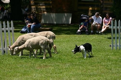
JOURNAL OF LATEX CLASS FILES, VOL. 6, NO. 1, JANUARY 2014                                                                 2

                                                                     max-pooling operation is carried out to fuse the
                                                                     outputs from the shared CNN into an integrative
                                                                     prediction. With max pooling, the high predictive
                                                                     scores from those hypotheses containing objects
                                                                     are reserved and the noisy ones are ignored.
                      Single-label images from ImageNet
                                                                     Therefore, as long as one hypothesis contains the
                                                                     object of interest, the noise can be suppressed
   horse&                                                            after the cross-hypothesis pooling. Redundant
   person
                                                                     hypotheses can also be well addressed by max
                                                                     pooling.

                                                                   • No explicit hypothesis label is required for training.
   dog&                                                              The state-of-the-art CNN models [15], [35]
   person
                                                                     utilize the hypothesis label for training. They
                                                                     first compute the Intersection-over-Union (IoU)
                      Multi-label images from Pascal VOC             overlap between hypotheses and ground-truth
                                                                     bounding boxes, and then assign the hypothesis
Fig. 1. Some examples from ImageNet [10] and Pascal                  with the label of the ground-truth bounding box
VOC 2007 [13]. The foreground objects in single-label                if their overlap is above a threshold. In contrast,
images are usually roughly aligned. However, the as-                 the proposed HCP takes an arbitrary number of
sumption of object alighment is not valid for multi-label            hypotheses as the inputs without any explicit
images. Also note the partial visibility and occlusion               hypothesis labels.
between objects in the multi-label images.
                                                                   • The shared CNN can be well pre-trained with a
                                                                     large-scale single-label image dataset. To address
data is required to cover the whole label space. For                 the problem of insufficient multi-label training
single-label images, it is practically easy to collect               images, based on the Hypotheses-CNN-Pooling
and annotate the images. However, the burden of                      architecture, the shared CNN can be first well
collection and annotation for a large scale multi-label              pre-trained on some large-scale single-label
image dataset is generally extremely high.                           dataset, e.g., ImageNet, and then fine-tuned on
   To address these issues and take full advantage                   the target multi-label dataset.
of CNN for multi-label image classification, in this
paper, we propose a flexible deep CNN structure,                   • The HCP outputs are intrinsically multi-label
called Hypotheses-CNN-Pooling (HCP). HCP takes                       prediction results. HCP produces a normalized
an arbitrary number of object segment hypotheses as                  probability distribution over the labels after the
the inputs, which may be generated by the sate-of-the-               softmax layer, and the the predicted probability
art objectiveness detection techniques, e.g., binarized              values are intrinsically the final classification
normed gradients (BING) [8], and then a shared CNN                   confidence values for the corresponding
is connected with each hypothesis. Finally the CNN                   categories.
output results from different hypotheses are aggre-
gated by max pooling to give the ultimate multi-                 Extensive experiments on two challenging multi-
label predictions. Particularly, the proposed HCP in-          label image datasets, Pascal VOC 2007 and VOC 2012,
frastructure possesses the following characteristics:          well demonstrate the superiority of the proposed
  • No ground-truth bounding box information is                HCP infrastructure over other state-of-the-arts. The
     required for training on the multi-label image dataset.   rest of the paper is organized as follows. We briefly
     Different from previous works [12], [5], [15],            review the related work of multi-label classification
     [35], which employ ground-truth bounding                  in Section 2. Section 3 presents the details of the
     box information for training, the proposed                HCP for image classification. Finally the experimental
     HCP requires no bounding box annotation.                  results and conclusions are provided in Section 4 and
     Since bounding box annotation is much more                Section 5, respectively.
     costly than labelling, the annotation burden is
     significantly reduced. Therefore, the proposed
     HCP has a better generalization ability when              2     R ELATED W ORK
     transferred to new multi-label image datasets.            During the past few years, many works on various
                                                               multi-label image classification models have been con-
  • The proposed HCP infrastructure is robust to the           ducted. These models are generally based on two
    noisy and/or redundant hypotheses. To suppress the         types of frameworks: bag-of-words (BoW) [19], [37],
    possibly noisy hypotheses, a cross-hypothesis              [6], [12], [5] and deep learning [35], [16], [38].
JOURNAL OF LATEX CLASS FILES, VOL. 6, NO. 1, JANUARY 2014                                                                                                                 3

                                                                                                                                            Scores for individual
                                                                                                                                                hypothesis

                                                                         Shared convolutional neural network

                     Hypotheses
                     extraction
                                                        5
                                                                          3
                                                                                           3             3
                                       11                   5                 3             3            3
                                                                     27             13            13           13                               …
                                                        55
  dog,person,sheep                                                                                                                          c                   Max
                                                                                          384          384          256
                              …

                                               227                 Max 256 Max                                            Max 4096 4096
                                                                                                                                                                Pooling
                                                                96 Pooling Pooling                                        Pooling

                                              cov1                cov2            cov3          cov4         cov5         fc6   fc7   fc8              fusion

Fig. 2. An illustration of the infrastructure of the proposed HCP. For a given multi-label image, a set of input
hypotheses to the shared CNN is selected based on the proposals generated by the state-of-the-art objectness
detection techniques, e.g., BING [8]. The shared CNN has a similar network structure to [24] except for the
layer fc8, where c is the category number of the target multi-label dataset. We feed the selected hypotheses into
the shared CNN and fuse the outputs into a c-dimensional prediction vector with cross-hypothesis max-pooling
operation. The shared CNN is firstly pre-trained on the single-label image dataset, e.g., ImageNet and then fine-
tuned with the multi-label images based on the squared loss function. Finally, we retrain the whole HCP to further
fine-tune the parameters for multi-label image classification.

2.1   Bag-of-Words Based Models                                               2.2        Deep Learning Based Models
                                                                              Deep learning tries to model the high-level abstrac-
                                                                              tions of visual data by using architectures com-
A traditional BoW model is composed of multiple                               posed of multiple non-linear transformations. Specif-
modules, e.g., feature representation, classification                         ically, deep convolutional neural network (CNN) [26]
and context modelling. For feature representation,                            has demonstrated an extraordinary ability for im-
the main components include hand-crafted feature                              age classification [21], [27], [29], [24], [30] on single-
extraction, feature coding and feature pooling, which                         label datasets such as CIFAR-10/100 [23] and Ima-
generate global representations for images. Specifi-                          geNet [10].
cally, hand-crafted features, such as SIFT [32], His-
                                                                                 More recently, CNN architectures have been
togram of Oriented Gradients [9] and Local Binary
                                                                              adopted to address multi-label problems. Gong et
Patterns [34] are firstly extracted on dense grids or
                                                                              al. [16] studied and compared several multi-label
sparse interest points and then quantized by different
                                                                              loss functions for the multi-label annotation problem
coding schemes, e.g., Vector Quantization [33], Sparse
                                                                              based on a similar network structure to [24]. However,
Coding [45] and Gaussian Mixture Models [20]. These
                                                                              due to the large number of parameters to be learned
encoded features are finally pooled by feature aggre-
                                                                              for CNN, an effective model requires lots of training
gation methods, such as Spatial Pyramid Matching
                                                                              samples. Therefore, training a task-specific convolu-
(SPM) [25], to form the image-level representation. For
                                                                              tional neural network is not applicable on datasets
classification, conventional models, such as SVM [4]
                                                                              with limited numbers of training samples.
and random forests [2], are utilized. Beyond conven-
                                                                                 Fortunately, some recent works [11], [15], [35], [40],
tional modelling methods, many recent works [19],
                                                                              [38], [17] have demonstrated that CNN models pre-
[42], [39], [6], [5] have demonstrated that the usage
                                                                              trained on large datasets with data diversity, e.g.,
of context information, e.g., spatial location of object
                                                                              ImageNet, can be transferred to extract CNN features
and background scene from the global view, can
                                                                              for other image datasets without enough training
considerably improve the performance of multi-label
                                                                              data. Pierre et al. [40] and Razavian et al. [38] proposed
classification and object detection.
                                                                              a CNN feature-SVM pipeline for multi-label classifi-
  Although these works have made great progress                               cation. Specifically, global images from a multi-label
in visual recognition tasks, the involved hand-crafted                        dataset are directly fed into the CNN, which is pre-
features are not always optimal for particular tasks.                         trained on ImageNet, to get CNN activations as the
Recently, in contrast to hand-crafted features, learnt                        off-the-shelf features for classification. However, dif-
features with deep learning structures have shown                             ferent from the single-label image, objects in a typical
great potential for various vision recognition tasks,                         multi-label image are generally less-aligned, and also
which will be introduced in the following subsection.                         often with partial visibility and occlusion as shown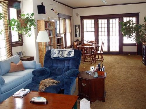
JOURNAL OF LATEX CLASS FILES, VOL. 6, NO. 1, JANUARY 2014                                                               4

in Figure 1. Therefore, global CNN features are not
optimal to multi-label problems. Recently, Oquab et
al. [35] and Girshick et al. [15] presented two proposal-
based methods for multi-label classification and detec-
tion. Although considerable improvements have been                       (a)                          (b)
made by these two approaches, these methods highly
                                                                                        C1:                     …
depend on the ground-truth bounding boxes, which
may limit their generalization ability when transferred
                                                                                        C2:                     …
to a new multi-label dataset without any bounding
box information.                                                                                                …
                                                                                        C3:
   In contrast, the proposed HCP infrastructure in this
paper requires no ground-truth bounding box infor-

                                                                                              …

                                                                                                  …

                                                                                                            …

                                                                                                                    …
mation for training and is robust to the possibly noisy                                 Cm:                     …

and/or redundant hypotheses. Different from [35],
                                                                         (c)                          (d)
[15], no explicit hypothesis label is required during
the training process. Besides, we propose a hypothesis      Fig. 3. (a) Source image. (b) Hypothesis bounding
selection method to select a small number of high-          boxes generated by BING. Different colors indicate
quality hypotheses (10 for each image) for training,        different clusters, which are produced by normalized
which is much less than the number used in [15]             cut. (c) Hypotheses directly generated by the bounding
(128 for each image), thus the training process is          boxes. (d) Hypotheses generated by the proposed HS
significantly sped up.                                      method.

3     H YPOTHESES -CNN-P OOLING                             Small number of hypotheses: Since all hypotheses
Figure 2 shows the architecture of the proposed             of a given multi-label image need to be fed into the
Hypotheses-CNN-Pooling (HCP) deep network. We               shared CNN simultaneously, more hypotheses cost
apply the state-of-the-art objectness detection tech-       more computational time and need more powerful
nique, i.e., BING [8], to produce a set of candidate        hardware (e.g., RAM and GPU). Thus a small hypoth-
object windows. A much smaller number of candi-             esis number is required for an effective hypotheses
date windows are then selected as hypotheses by the         extraction approach.
proposed hypotheses extraction method. The selected         High computational efficiency: As the first step of
hypotheses are fed into a shared convolutional neural       the proposed HCP, the efficiency of hypotheses ex-
network (CNN). The confidence vectors from the in-          traction will significantly influence the performance
put hypotheses are combined through a fusion layer          of the whole framework. With high computational
with max pooling operation, to generate the ultimate        efficiency, HCP can be easily integrated into real-time
multi-label predictions. In specific, the shared CNN        applications.
is first pre-trained on a large-scale single-label image       In summary, a good hypothesis generating algo-
dataset, i.e., ImageNet and then fine-tuned on the          rithm should generate as few hypotheses as possible
target multi-label dataset, e.g., Pascal VOC, by using      in an efficient way and meanwhile achieve as high
the entire image as the input. After that, we retrain       recall rate as possible.
the proposed HCP with a squared loss function for              During the past few years, many methods [31],
the final prediction.                                       [7], [46], [1], [3], [43] have been proposed to tackle
                                                            the hypotheses detection problem. [31], [7], [46] are
                                                            based on salient object detection, which try to detect
3.1   Hypotheses Extraction                                 the most attention-grabbing (salient) object in a given
HCP takes an arbitrary number of object segment             image. However, these methods are not applicable
hypotheses as the inputs to the shared CNN and              to HCP, since saliency based methods are usually
fuses the prediction of each hypothesis with the max        applied to a single-label scheme while HCP is a multi-
pooling operation to get the ultimate multi-label pre-      label scheme. [1], [3], [43] are based on objectness pro-
dictions. Therefore, the performance of the proposed        posal (hypothesis), which generate a set of hypotheses
HCP largely depends on the quality of the extracted         to cover all independent objects in a given image. Due
hypotheses. Nevertheless, designing an effective hy-        to the large number of proposals, such methods are
potheses extraction approach is challenging, which          usually quite time-consuming, which will affect the
should satisfy the following criteria:                      real-time performance of HCP.
High object detection recall rate: The proposed HCP            Most recently, Cheng et al. [8] proposed a surpris-
is based on the assumption that the input hypotheses        ingly simple and powerful feature called binarized
can cover all single objects of the given multi-label       normed gradients (BING) to find object candidates by
image, which requires a high detection recall rate.         using objectness scores. This method is faster (300fps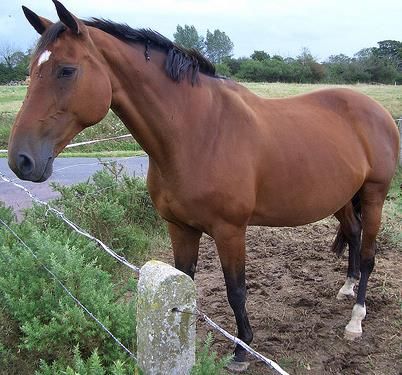
JOURNAL OF LATEX CLASS FILES, VOL. 6, NO. 1, JANUARY 2014                                                                              5

on a single laptop CPU) than most popular alter-                    Single-label Images
                                                                                            Pre-training on single-label image set
natives [1], [3], [43] and has a high object detection                (e.g. ImageNet)

recall rate (96.2% with 1,000 hypotheses). Although
the number of hypotheses (i.e., 1,000) is very small                  …
compared with a common sliding window paradigm,
it is still very large for HCP.
                                                                    Step1
   To address this problem, we propose a hypotheses                                                      Parameters transferring
selection (HS) method to select hypotheses from the                 Multi-label Images
                                                                    (e.g. Pascal VOC)
proposals extracted by BING. A set of hypothesis
bounding boxes are produced by BING for a given                       …
image, denoted by H = {h1 , h2 , ..., hn }, where n is
the hypothesis number. An n × n affinity matrix W is
constructed, where Wij (i, j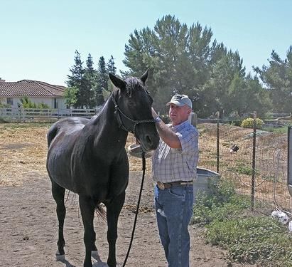
JOURNAL OF LATEX CLASS FILES, VOL. 6, NO. 1, JANUARY 2014                                                                    6

is not equal to that of ImageNet, the output of the                 possible diversified objects. However, with more hy-
last fully-connected layer is fed into a c-way softmax              potheses, noise (hypotheses covering no object) will
which produces a probability distribution over the c                inevitably increase.
class labels. Different from the pre-training, squared                 To suppress the possibly noisy hypotheses, a cross-
loss is used during I-FT. Suppose there are N images                hypothesis max-pooling is carried out to fuse the out-
in the multi-label image set, and yi = [yi1 , yi2 , · · · , yic ]   puts into one integrative prediction. Suppose vi (i =
is the label vector of the ith image. yij = 1 (j =                  1, ..., l) is the output vector of the ith hypothesis from
1, · · · , c) if the image is annotated with class j, and                                        (j)
                                                                    the shared CNN and vi (j = 1, . . . , c) is the j th
otherwise yij = 0. The ground-truth probability vector              component of vi . The cross-hypothesis max-pooling
of the ith image is defined as p̂i = yi /||yi ||1 and the           in the fusion layer can be formulated as
predictive probability vector is pi = [pi1 , pi2 , · · · , pic ].
                                                                                               (j)   (j)      (j)
And then the cost function to be minimized is defined                           v (j) = max(v1 , v2 , . . . , vl ),        (3)
as
                          N    c                                    where v (j) can be considered as the predicted value
                       1 XX                   2
                   J=            (pik − p̂ik ) .             (2)    for the j th category of the given image.
                       N i=1                                           The cross-hypothesis max-pooling is a crucial step
                              k=1
                                                                    for the whole HCP framework to be robust to the
During the I-FT process, as shown in Figure 4, the pa-              noise. If one hypothesis contains an object, the output
rameters of the first seven layers are initialized by the           vector will have a high response (i.e., large value)
parameters pre-trained on ImageNet and the param-                   on the j th component, meaning a high confidence for
eters of the last fully-connected layer are randomly                the corresponding j th category. With cross-hypothesis
initialized with a Gaussian distribution G(µ, σ)(µ =                max-pooling, large predicted values corresponding to
0, σ = 0.01). The learning rates of the convolutional               objects of interest will be reserved, while the values
layers, the first two fully-connected layers and the                from the noisy hypotheses will be ignored.
last fully-connected layer are initialized as 0.001, 0.002
                                                                       During the hypotheses-fine-tuning (H-FT) process,
and 0.01 at the beginning, respectively. We executed
                                                                    the output of the fusion layer is fed into a c-way
60 epoches in total and decreased the learning rate
                                                                    softmax layer with the squared loss as the cost func-
to one tenth of the current rate of each layer after 20
                                                                    tion, which is defined as Eq. (2). Similar as I-FT, we
epoches (momentum=0.9, weight decay=0.0005).
                                                                    also adopt a discriminating learning rate scheme for
   By setting the different learning rates for different            different layers. Specifically, we execute 60 epoches in
layers, the updating rates for the parameters from                  total and empirically set the learning rates of the con-
different layers also vary. The first few convolutional             volutional layers, the first two fully-connected layers
layers mainly extract some low-level invariant repre-               and the last fully-connected layer as 0.0001, 0.0002,
sentations, thus the parameters are quite consistent                0.001 at the beginning, respectively. We decrease the
from the pre-trained dataset to the target dataset,                 learning rates to one tenth of the current ones after
which is achieved by a very low learning rate (i.e.,                every 20 epoches. The momentum and the weight
0.001). Nevertheless, in the final layers of the network,           decay are set as 0.9 and 0.0005, which are the same as
especially the last fully-connected layer, which are                in the I-FT step.
specifically adapted to the new target dataset, a much
higher learning rate is required to guarantee a fast
convergence to the new optimum. Therefore, the pa-                  3.4   Multi-label Classification for Test Image
rameters can better adapt to the new dataset without
                                                                    Based on the trained HCP model, the multi-label
clobbering the pre-trained initialization. It should be
                                                                    classification of a given image can be summarized as
noted that the I-FT is a critical step of HCP. We tried
                                                                    follows. We firstly generate the input hypotheses of
without this step and found that the performance on
                                                                    the given image based on the proposed HS method.
VOC 2007 dropped dramatically.
                                                                    Then, for each hypothesis, a c-dimensional predictive
                                                                    result can be obtained by the shared CNN. Finally, we
                                                                    utilize the cross-hypothesis max-pooling operation to
3.3   Hypotheses-fine-tuning
                                                                    produce the final prediction. As shown in Fig. 5, the
All the l = mk hypotheses are fed into the shared                   second row and the third row indicate the generated
CNN, which has been initialized as elaborated in Sec-               hypotheses and the corresponding outputs from the
tion 3.2. For each hypothesis, a c-dimensional vector               shared CNN. For each object independent hypothesis,
can be computed as the output of the shared CNN.                    there is a high response on the corresponding cate-
Indeed, the proposed HCP is based on the assumption                 gory (e.g., for the first hypothesis, the response on
that each hypothesis contains at most one object and                car is very high). After cross-hypothesis max-pooling
all the possible objects are covered by some subset                 operation, as indicated by the last row in Fig. 5, the
of the extracted hypotheses. Therefore, the number                  high responses (i.e., car, horse and person), which can
of hypotheses should be large enough to cover all                   be considered as the predicted labels, are reserved.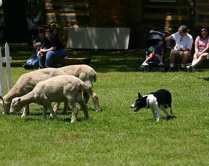
JOURNAL OF LATEX CLASS FILES, VOL. 6, NO. 1, JANUARY 2014                                                                       7

                                                                           based on hand-crafted features and those based on
                                                                           learnt features.

                                            Generate hypotheses             • INRIA [19]: Harzallah et al. proposed a
                                                                              contextual combination method of localization
                                                                              and classification to improve the performance
                                                                       …      for both. Specifically, for classification, image
                                                                              representation is built on the traditional feature
                                            Input the shared CNN              extraction-coding-pooling pipeline, and object
                                                                              localization is built on sliding-widow approaches.
                                                                       …      Furthermore, the localization is employed to
                                   person
      car

                                                    person
                     horse

                                                                              enhance the classification performance.
                                            Cross-hypothesis max-pooling
                                                                            • FV [37]: The Fisher Vector representation of
                                                                              images can be considered as an extension of the
                                                                              bag-of-words. Some well-motivated strategies,
                                                                              e.g., L2 normalization, power normalization and
                                                                              spatial pyramids, are adopted over the original
                             car

                                   horse
                                   person

                                                                              Fisher Vector to boost the classification accuracy.

Fig. 5. An illustration of the proposed HCP for a VOC                       • NUS: In [5], Chen et al. presented an Ambiguity-
2007 test image. The second row indicates the gener-                          guided Mixture Model (AMM) to seamlessly
ated hypotheses. The third row indicate the predicted                         integrate external context features and object
results for the input hypotheses. The last row is pre-                        features for general classification, and then the
dicted result for the test image after cross-hypothesis                       contextualized SVM was further utilized to
max-pooling operation.                                                        iteratively and mutually boost the performance
                                                                              of object classification and detection tasks.
                                                                              Dong et al. [12] proposed an Ambiguity
4       E XPERIMENTAL R ESULTS                                                Guided Subcategory (AGS) mining approach,
In this section, we present the experiments to validate                       which can be seamlessly integrated into an
the effectiveness of our proposed Hypotheses-CNN-                             effective subcategory-aware object classification
Pooling (HCP) framework for multi-label image clas-                           framework, to improve both detection and
sification.                                                                   classification performance. The combined
                                                                              version of the above two, NUS-PSL [47] received
                                                                              the winner prizes of the classification task in
4.1         Datasets and Settings                                             PASCAL VOC 2010-2012.
We evaluate the proposed HCP on the PASCAL Vi-
sual Object Classes Challenge (VOC) datasets [13],                          • CNN-SVM [38]: OverFeat [40], which obtained
which are widely used as the benchmark for multi-                             very competitive performance in the image
label classification. In this paper, PASCAL VOC 2007                          classification task of ILSVRC 2013, was released
and VOC 2012 are employed for experiments. These                              by Sermanet et al. as a feature extractor.
two datasets, which contain 9,963 and 22,531 images                           Razavian et al. [38] employed OverFeat, which is
respectively, are divided into train, val and test subsets.                   pre-trained on ImageNet, to get CNN activations
We conduct our experiments on the trainval/test splits                        as the off-the-shelf features. The state-of-the-art
(5,011/4,952 for VOC 2007 and 11,540/10,991 for VOC                           classification result on PASCAL VOC 2007 was
2012). The evaluation metric is Average Precision (AP)                        achieved by using linear SVM classifiers over
and mean of AP (mAP) complying with the PASCAL                                the 4,096 dimensional feature representation
challenge protocols.                                                          extracted from the 22nd layer of OverFeat.
   Instead of using two GPUs as in [24], we conduct
experiments on one NVIDIA GTX Titan GPU with                                • I-FT: The structure of the shared CNN follows
6GB memory and all our training algorithms are                                that of Krizhevsky et al. [24]. The shared CNN
based on the code provided by Jia et al. [22]. The                            was first pre-trained on ImageNet, and then
initialization of the shared CNN is based on the                              the last fully-connected layer was modified into
parameters pre-trained on the 1,000 classes and 1.2                           4096×20, and the shared CNN was re-trained
million images of ILSVRC-2012.                                                with squared loss function on PASCAL VOC for
   We compare the proposed HCP with the state-of-                             multi-label classification.
the-art approaches. Specifically, the competing algo-
rithms are generally divided into two types: those                          • PRE-1000C and PRE-1512 [35]: Oquab et al. pro-
JOURNAL OF LATEX CLASS FILES, VOL. 6, NO. 1, JANUARY 2014                                                                                     8

                                                                    with that using all categories (all the 20 categories in
                                                                    PASCAL VOC) for training.
                                                                       Since the proposed HCP is independent of the
       goldfish         ray            frog      American lobster   ground-truth bounding box, no object location in-
                                                                    formation can be used for training. Inspired by the
                                                                    generalization ability test in [8], the detection dataset
                                                                    of ILSVRC 2013 is used as augmented data for BING
         fox            seal        loggerhead      cottontail      training. It contains 395,909 training images with
                                                                    ground-truth bounding box annotation from 200 cat-
                                                                    egories. To validate the generalization ability of the
                                                                    proposed framework for other multi-label datasets,
                                                                    the categories as well as their subcategories which
        snail        corkscrew         cot        cheeseburger
                                                                    are semantically overlapping with the PASCAL VOC
                                                                    categoires are removed2 .
                                                                       For a fair comparison, we follow [8] and only use
                                                                    randomly 13,894 images (instead of all images) from
      cucumber         bagel          mug           bell pepper
                                                                    the detection dataset of ILSVRC 2013 for model train-
                                                                    ing. Some selected samples are illustrated in Figure 6,
Fig. 6. Exemplar images with ground-truth bounding
                                                                    from which we can see that there are big differences
boxes from the detection dataset of ILSVRC 2013.
                                                                    between objects in PASCAL VOC and the selected
                                                                    ImageNet samples. After training, the learnt BING-
      posed to transfer image representations learned               ImageNet model is used to produce hypotheses for
      with CNN on ImageNet to other visual recog-                   VOC 2007 and VOC 2012. We test the object detection
      nition tasks with limited training data. The net-             rate with 1000 proposals on VOC 2007, which is only
      work has exactly the same architecture as in [24].            0.3% lower than the reported result (i.e., 96.2%) in [8].
      Firstly, the network is pre-trained on ImageNet.                 Considering the computational time and the limita-
      Then the first seven layers of CNN are fixed                  tion of hardware, we proposed a hypotheses selection
      with the pre-trained parameters and the last                  (HS) method to filter the input hypotheses produced
      fully-connected layer is replaced by two adap-                by BING-ImageNet. As elaborated in Section 3.1, we
      tation layers. Finally, the adaptation layers are             cluster the extracted proposals into 10 clusters based
      trained with images from the target PASCAL                    on their bounding box overlapping information by
      VOC dataset. PRE-1000C and PRE-1512 mean                      normalized-cut [41]. The hypotheses are filtered out,
      the transferred parameters are pre-trained on the             which have smaller areas than 900 pixels or larger
      original ImageNet dataset with 1000 categories                height/width (or width/height) ratios than 4. Some
      and the augmented one with 1512 categories,                   exemplar hypotheses extracted by the proposed HS
      respectively. For PRE-1000C, 1.2 million images               method are shown in Figure 7. We sort the hypotheses
      from ILSVRC-2012 are employed to pre-train the                for each cluster based on the predicted objectness
      CNN, while for PRE-1512, 512 additional Ima-                  scores and show the first five hypotheses.
      geNet classes (e.g., furniture, motor vehicle, bicy-             During the training step, for each training image,
      cle etc.) are augmented to increase the semantic              the top k hypotheses from each cluster are selected
      overlap with categories in PASCAL VOC. To                     and fed into the shared CNN. We experimentally vary
      accommodate the larger number of classes, the                 k = 1, 2, 3, 4, 5 to train the proposed HCP on VOC
      dimensions of the first two fully-connected layers            2007 and observe that the performance changes only
      are increased from 4,096 to 6,144.                            slightly on the testing dataset. Therefore, we set k = 1
                                                                    (i.e., 10 hypotheses for each image) for both VOC 2007
4.2    Hypotheses Extraction                                        and VOC 2012 during the training stage to reduce
                                                                    the training time. To achieve high object recall rate,
In [8], BING1 has shown a good generalization abil-                 500 hypotheses (i.e., k = 50) are extracted from each
ity on the images containing object categories that                 test image during the testing stage. On VOC 2012, the
are not used for training. Specifically, [8] trained a              hypotheses-fine-tuning step takes roughly 20 hours.
linear SVM using 6 object categories (i.e., the first 6             For each testing image, about 1.5 second is cost.
categories in VOC dataset according to alpha order)
and the remaining 14 categories were used for testing.
The experimental results in [8] demonstrate that the
                                                                      2. The removed categories include bicycle, bird, water bottle, bus,
transferred model almost has the same performance                   car, domestic cat, chair, table, dog, horse, motorcycle, person, flower pot,
                                                                    sheep, sofa, train, tv or monitor, wine bottle, watercraft, unicycle, cattle
  1. http://mmcheng.net/bing/                                       and cart.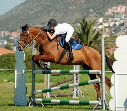
JOURNAL OF LATEX CLASS FILES, VOL. 6, NO. 1, JANUARY 2014                                                     9

                         C1:                                    C2:

                         C3:                                    C4:

                         C5:                                    C6:

   dog, horse, person    C7:                                    C8:

                         C9:                                   C10:

                         C1:                                    C2:

                         C3:                                    C4:

                         C5:                                    C6:

   cat, person, plant,
                         C7:                                    C8:
   sofa

                         C9:                                   C10:

                         C1:                                    C2:

                         C3:                                    C4:

                         C5:                                    C6:

   cat, chair, table,    C7:                                    C8:
   plant, sofa

                         C9:                                   C10:

Fig. 7. Exemplar hypotheses extracted by the proposed HS method. For each image, the ground-truth bounding
boxes are shown on the left and the corresponding hypotheses are shown on the right. C1-C10 are the 10
clusters produced by normalized-cut [41] and hypotheses in the same cluster share similar location information.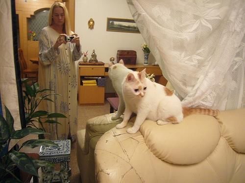
JOURNAL OF LATEX CLASS FILES, VOL. 6, NO. 1, JANUARY 2014                                                                                     10

                 0.15
                                                                 2007, which is more competitive than the scheme of
                 0.14                                            CNN features with SVM classifier [38].
                 0.13

                 0.12                                            4.4    Image Classification Results
  squared loss

                 0.11
                                                                 Image Classification on VOC 2007: Table 1 reports
                  0.1                                            our experimental results compared with the state-of-
                 0.09
                                                                 the-arts on VOC 2007. The upper part of Table 1 shows
                                                                 the methods not using ground-truth bounding box
                 0.08
                                                                 information for training, while the lower part of the
                 0.07
                                                                 table shows the methods with that information. Be-
                 0.06
                        0                                   60
                                                                 sides, CNN-SVM, I-FT, HCP-1000C, HCP-2000C and
                                                epoch
                                                                 PRE-1000C are methods using additional images for
Fig. 8. The changing trend of the squared loss during            training from an extra dataset, i.e., ImageNet, and
the I-FT step on VOC 2007.                                       the other methods only utilize PASCAL VOC data
                                                                 for training. In specific, HCP-1000C indicates that the
                 0.75
                                                                 initialized parameters of the shared CNN are pre-
                                                                 trained on the 1.2 million images from 1000 categories
                 0.74
                                                                 of ILSVRC-2012. Similar as [35], for HCP-2000C, we
                 0.73
                                                                 augment the ILSVRC-2012 training set with additional
                 0.72                                            1,000 ImageNet classes (about 0.8 million images)
                 0.71                                            to improve the semantic overlap with classes in the
 mAP

                                                                 Pascal VOC dataset.
                  0.7
                                                                    From the experimental results, we can see that the
                 0.69
                                                                 CNN based methods which utilize additional im-
                 0.68                                            ages from ImageNet have a 2.6%∼13.9% improvement
                 0.67                                            compared with the state-of-the-art methods based on
                 0.66
                                                                 hand-crafted features, i.e., 71.3% [5]. By utilizing the
                        0                                   60
                                                epoch            ground-truth bounding box information, a remarkable
                                                                 improvement can be achieved for both deep learn-
Fig. 9. The changing trend of mAP scores during the              ing based methods (PRE-1000C vs. CNN-SVM and
I-FT step on VOC 2007. The mAP converges fast to                 I-FT) and hand-crafted feature based methods (AGS
74.4% after almost 15 epoches on test dataset.                   and AMM vs. INRIA and FV). However, bounding
                                                                 box annotation is quite costly. Therefore, approaches
                                                                 requiring ground-truth bounding boxes cannot be
4.3                     Initialization of HCP                    transferred to the datasets without such annotation.
As discussed in Section 3.2, the initialization pro-             From Table 1, it can be seen that the proposed HCP
cess of HCP consists of two steps: Pre-training and              has a significant improvement compared with the
Image-fine-tuning (I-FT). Since the structure setting            state-of-the-art performance even without bounding
of the shared-CNN is almost consistent with the pre-             box annotation i.e., 81.5% vs. 77.7% (HCP-1000C vs.
trained model implemented by [22], we apply the pre-             PRE-1000C [35]). Compared with HCP-1000C, 3.7%
trained model on ImageNet by [22] to initialize the              improvement can be achieved by HCP-2000C. Since
convolutional layers and the first two fully-connected           the proposed HCP requires no bounding box anno-
layers of the shared CNN. For I-FT, we use images                tation, the proposed method has a much stronger
from PASCAL VOC to re-train the shared CNN. As                   generalization ability to new multi-label datasets.
shown in Figure 4, the pre-trained parameters for                   Figure 10 shows the predicted scores of images for
the first seven layers are transferred to initialize the         different categories on the VOC 2007 testing dataset
CNN for fine-tuning. The last fully-connected layer              using models from different fine-tuning epoches. For
with 4096×20 parameters is randomly initialized with             each histogram3 , orange bars indicate predicted scores
Gaussian distribution.                                           of the ground-truth categories. We show the predic-
   Actually, similar as Gong et al. [16], the class la-          tive scores at the 1st and the 60th epoch during I-
bels of a given image can also be predicted by the               FT and H-FT stages. For the first row, it can be
fine-tuned model at the I-FT stage. Figure 8 shows               seen that the predictive score for the train category
the changing trends of the squared loss of different             gradually increases. Besides, for the third row, it can
epoches on VOC 2007 during I-FT. The corresponding               be seen that there are three ground-truth categories
change of mAP score on the test dataset is shown in
                                                                    3. For each histogram, categories from left to right are plane, bike,
Figure 9. We can see that the mAP score based on the             bird, boat, bottle, bus, car, cat, chair, cow, table, dog, horse, motor, person,
image-fine-tuned model can achieve 74.4% on VOC                  plant, sheep, sofa, train and tv.
JOURNAL OF LATEX CLASS FILES, VOL. 6, NO. 1, JANUARY 2014 11
TABLE 1
Classification results (AP in %) comparison for state-of-the-art approaches on VOC 2007 (trainval/test). The
upper part shows methods not using ground-truth bounding box information for training, while the lower part
shows methods with that information. * indicates methods using additional data (i.e., ImageNet) for training.
plane bike bird boat bottle bus car cat chair cow table dog horse motor person plant sheep sofa train tv mAP
INRIA[19] 77.2 69.3 56.2 66.6 45.5 68.1 83.4 53.6 58.3 51.1 62.2 45.2 78.4 69.7 86.1 52.4 54.4 54.3 75.8 62.1 63.5
FV[37] 75.7 64.8 52.8 70.6 30.0 64.1 77.5 55.5 55.6 41.8 56.3 41.7 76.3 64.4 82.7 28.3 39.7 56.6 79.7 51.5 58.3
CNN-SVM*[38] 88.5 81.0 83.5 82.0 42.0 72.5 85.3 81.6 59.9 58.5 66.5 77.8 81.8 78.8 90.2 54.8 71.1 62.6 87.4 71.8 73.9
I-FT* 91.4 84.7 87.5 81.8 40.2 73.0 86.4 84.8 51.8 63.9 67.9 82.7 84. 0 76.9 90.4 51.5 79.9 54.1 89.5 65.8 74.4
HCP-1000C* 95.1 90.1 92.8 89.9 51.5 80.0 91.7 91.6 57.7 77.8 70.9 89.3 89.3 85.2 93.0 64.0 85.7 62.7 94.4 78.3 81.5
HCP-2000C* 96.0 92.1 93.7 93.4 58.7 84.0 93.4 92.0 62.8 89.1 76.3 91.4 95.0 87.8 93.1 69.9 90.3 68.0 96.8 80.6 85.2
plane bike bird boat bottle bus car cat chair cow table dog horse motor person plant sheep sofa train tv mAP
AGS[12] 82.2 83.0 58.4 76.1 56.4 77.5 88.8 69.1 62.2 61.8 64.2 51.3 85.4 80.2 91.1 48.1 61.7 67.7 86.3 70.9 71.1
AMM[5] 84.5 81.5 65.0 71.4 52.2 76.2 87.2 68.5 63.8 55.8 65.8 55.6 84.8 77.0 91.1 55.2 60.0 69.7 83.6 77.0 71.3
PRE-1000C*[35] 88.5 81.5 87.9 82.0 47.5 75.5 90.1 87.2 61.6 75.7 67.3 85.5 83.5 80.0 95.6 60.8 76.8 58.0 90.4 77.9 77.7
TABLE 2
Classification results (AP in %) comparison for state-of-the-art approaches on VOC 2012 (trainval/test). The
upper part shows methods not using ground-truth bounding box information for training, while the lower part
shows methods with that information. * indicates methods using additional data (i.e., ImageNet) for training.
plane bike bird boat bottle bus car cat chair cow table dog horse motor person plant sheep sofa train tv mAP
I-FT* 94.6 74.3 87.8 80.2 50.1 82.0 73.7 90.1 60.6 69.9 62.7 86.9 78.7 81.4 90.5 45.9 77.5 49.3 88.5 69.2 74.7
LeCun-ICML*[28] 96.0 77.1 88.4 85.5 55.8 85.8 78.6 91.2 65.0 74.4 67.7 87.8 86.0 85.1 90.9 52.2 83.6 61.1 91.8 76.1 79.0
HCP-1000C* 97.7 83.0 93.2 87.2 59.6 88.2 81.9 94.7 66.9 81.6 68.0 93.0 88.2 87.7 92.7 59.0 85.1 55.4 93.0 77.2 81.7
HCP-2000C* 97.5 84.3 93.0 89.4 62.5 90.2 84.6 94.8 69.7 90.2 74.1 93.4 93.7 88.8 93.3 59.7 90.3 61.8 94.4 78.0 84.2
plane bike bird boat bottle bus car cat chair cow table dog horse motor person plant sheep sofa train tv mAP
NUS-PSL[47] 97.3 84.2 80.8 85.3 60.8 89.9 86.8 89.3 75.4 77.8 75.1 83.0 87.5 90.1 95.0 57.8 79.2 73.4 94.5 80.7 82.2
PRE-1000C*[35] 93.5 78.4 87.7 80.9 57.3 85.0 81.6 89.4 66.9 73.8 62.0 89.5 83.2 87.6 95.8 61.4 79.0 54.3 88.0 78.3 78.7
PRE-1512*[35] 94.6 82.9 88.2 84.1 60.3 89.0 84.4 90.7 72.1 86.8 69.0 92.1 93.4 88.6 96.1 64.3 86.6 62.3 91.1 79.8 82.8
HCP-2000C+NUS-PSL* 98.9 91.8 94.8 92.4 72.6 95.0 91.8 97.4 85.2 92.9 83.1 96.0 96.6 96.1 94.9 68.4 92.0 79.6 97.3 88.5 90.3
in the given image, i.e., car, horse, person. It should be the integrative result, while the proposed HCP-1000C
noted that the car category is not detected during fine- is based on a single model without any fusion. For
tuning while it is successfully recovered in HCP. This PRE-1512, 512 extra ImageNet classes are selected for
may be because the proposed HCP is a hypotheses CNN pre-training. In addition, the selected classes
based method and both foreground (i.e., horse, person) have intensive semantic overlap with PASCAL VOC,
and background (i.e., car) objects can be equivalently including hoofed mammal, furniture, motor vehicle, public
treated. However, during the fine-tuning stage, the transport, bicycle. Therefore, the greater improvement
entire image is treated as the input, which may lead of PRE-1512 compared with HCP-1000C is reasonable.
to ignorance of some background categories. By augmenting another 1,000 classes, our proposed
Image Classification on VOC 2012: Table 2 reports HCP-2000C can achieve an improvement of 1.4% com-
our experimental results compared with the state-of- pared with PRE-1512.
the-arts on VOC 2012. LeCun et al. [28] reported the Finally, the comparison in terms of rigid and ar-
classification results on VOC 2012, which achieved ticulated categories among NUS-PSL, PRE-1512 and
the state-of-the-art performance without using any HCP-2000C is shown in Table 3, from which it can be
bounding box annotation. Compared with [28], the seen that the hand-crafted feature based scheme, i.e.,
proposed HCP-1000C has an improvement of 2.7%. NUS-PSL, outperforms almost all CNN feature based
Both pre-trained on the ImageNet dataset with 1,000 schemes for rigid categories, including plane, bike, boat,
classes, HCP-1000C gives a more competitive result bottle, bus, car, chair, table, motor, sofa, train, tv, while
compared with PRE-1000C [35] (81.7% vs. 78.7%). for articulated categories, CNN feature based schemes
From Table 2, it can be seen that the proposed HCP- seem to be more powerful. Based on theses results, it
1000C is not as competitive as NUS-PSL [47] and PRE- can be observed that there is strong complementar-
1512 [35]. This can be explained as follows. For NUS- ity between hand-crafted feature based schemes and
PSL, which got the winner prize of the classification CNN feature based schemes. To verify this assump-
task in PASCAL VOC 2012, model fusion from both tion, a late fusion between the predicted scores of
detection and classification is employed to generate NUS-PSL (also from the authors of this paper) andJOURNAL OF LATEX CLASS FILES, VOL. 6, NO. 1, JANUARY 2014 12
I-FT-1 st epoch I-FT-60 th epoch H-FT-1 st epoch H-FT-60 th epoch
1 1 1 1
0.8 0.8 0.8 0.8
0.6 0.6 0.6 0.6
0.4 0.4 0.4 0.4
0.2 0.2 0.2 0.2
train
0 0 0 0
1 1 1 1
0.8 0.8 0.8 0.8
0.6 0.6 0.6 0.6
0.4 0.4 0.4 0.4
0.2 0.2 0.2 0.2
horse, person
0 0 0 0
1 1 1 1
0.8 0.8 0.8 0.8
0.6 0.6 0.6 0.6
0.4 0.4 0.4 0.4
0.2 0.2 0.2 0.2
car, horse, person
0 0 0 0
1 1 1 1
0.8 0.8 0.8 0.8
0.6 0.6 0.6 0.6
0.4 0.4 0.4 0.4
0.2 0.2 0.2 0.2
bike, bus, car,
0 0 0 0
person
1 1 1 1
0.8 0.8 0.8 0.8
0.6 0.6 0.6 0.6
0.4 0.4 0.4 0.4
0.2 0.2 0.2 0.2
bottle, chair, table, 0 0 0 0
person, plant
Fig. 10. Samples of predicted scores on the VOC 2007 testing dataset using models from different fine-tuning
epochs (i.e., I-FT-1st epoch, I-FT-60th epoch, H-FT-1st epoch, and H-FT-60th epoch).
HCP is executed to make an enhanced prediction that late fusion between outputs of CNN and hand-
for VOC 2012. Incredibly, the mAP score on VOC crafted feature schemes can incredibly enhance the
2012 can surge to 90.3% as shown in Table 2, which classification performance.
demonstrates the great complementarity between the
plane
bike
bird
boat
bottle
bus
car
cat
chair
cow
table
dog
horse
motor
person
plant
sheep
sofa
train
tv
traditional framework and the deep networks. R EFERENCES
[1] B. Alexe, T. Deselaers, and V. Ferrari. Measuring the objectness
of image windows. IEEE Trans. Pattern Analysis and Machine
5 C ONCLUSIONS Intelligence, 34(11):2189–2202, 2012.
[2] L. Breiman. Random forests. Machine learning, 45(1):5–32, 2001.
[3] J. Carreira and C. Sminchisescu. Cpmc: Automatic object
In this paper, we presented a novel Hypotheses- segmentation using constrained parametric min-cuts. IEEE
CNN-Pooling (HCP) framework to address the multi- Trans. Pattern Analysis and Machine Intelligence, 34(7):1312–1328,
2012.
label image classification problem. Based on the pro- [4] C.-C. Chang and C.-J. Lin. Libsvm: a library for support
posed HCP, CNN pre-trained on large-scale single- vector machines. ACM Trans. Intelligent Systems and Technology,
label image datasets, e.g., ImageNet, can be success- 2(3):27, 2011.
[5] Q. Chen, Z. Song, J. Dong, Z. Huang, Y. Hua, and S. Yan.
fully transferred to tackle the multi-label problem. In Contextualizing object detection and classication. IEEE Trans.
addition, the proposed HCP requires no bounding box Pattern Analysis and Machine Intelligence, 2014.
[6] Q. Chen, Z. Song, Y. Hua, Z. Huang, and S. Yan. Hierarchical
annotation for training, and thus can easily adapt to matching with side information for image classification. In
new multi-label datasets. We evaluated our method Computer Vision and Pattern Recognition, pages 3426–3433, 2012.
on VOC 2007 and VOC 2012, and verified that signif- [7] M.-M. Cheng, J. Warrell, W.-Y. Lin, S. Zheng, V. Vineet, and
N. Crook. Efficient salient region detection with soft image
icant improvement can be made by HCP compared abstraction. In International Conference on Computer Vision,
with the state-of-the-arts. Furthermore, it is proved pages 1529–1536, 2013.JOURNAL OF LATEX CLASS FILES, VOL. 6, NO. 1, JANUARY 2014 13
TABLE 3
Comparison in terms of rigid categories and articulated categories among NUS-PSL, PRE-1512 and
HCP-2000C.
Comparison
class
NUS-PSL PRE-1512 HCP-2000C NUS-PSL vs. PRE-1512 mean NUS-PSL vs. HCP-2000C mean
plane 97.3 94.6 97.5 2.7 -0.2
bike 84.2 82.9 84.3 1.3 -0.1
boat 85.3 84.1 89.4 1.2 -4.1
bottle 60.8 60.3 62.5 0.5 -1.7
bus 89.9 89.0 90.2 0.9 -0.3
car 86.8 84.4 84.6 2.4 2.2
Rigid 3.0 1.5
chair 75.4 72.1 69.7 3.3 5.7
table 75.1 69.0 74.1 6.1 1.0
motor 90.1 88.6 88.8 1.5 1.3
sofa 73.4 62.3 61.8 11.1 11.6
train 94.5 91.1 94.4 3.4 0.1
tv 80.7 79.8 78.0 0.9 2.7
bird 80.8 88.2 93.0 -7.4 -12.2
cat 89.3 90.7 94.8 -1.4 -5.5
cow 77.8 86.8 90.2 -9.0 -12.4
Articulated dog 83.0 92.1 93.4 -9.1 -5.9 -10.4 -7.1
horse 87.5 93.4 93.7 -5.9 -6.2
person 95.0 96.1 93.3 -1.1 1.7
sheep 79.2 86.6 90.3 -7.4 -11.1
plant 57.8 64.3 59.7 -7.4 -0.9
[8] M.-M. Cheng, Z. Zhang, W.-Y. Lin, and P. H. S. Torr. BING: Bi- of features from tiny images. Computer Science Department,
narized normed gradients for objectness estimation at 300fps. University of Toronto, Tech. Rep, 2009.
In Computer Vision and Pattern Recognition, 2014. [24] A. Krizhevsky, I. Sutskever, and G. Hinton. Imagenet classi-
[9] N. Dalal and B. Triggs. Histograms of oriented gradients for fication with deep convolutional neural networks. In Neural
human detection. In Computer Vision and Pattern Recognition, Information Processing Systems, pages 1106–1114, 2012.
volume 1, pages 886–893, 2005. [25] S. Lazebnik, C. Schmid, and J. Ponce. Beyond bags of features:
[10] J. Deng, W. Dong, R. Socher, L.-J. Li, K. Li, and L. Fei- Spatial pyramid matching for recognizing natural scene cate-
Fei. Imagenet: A large-scale hierarchical image database. In gories. In Computer Vision and Pattern Recognition, volume 2,
Computer Vision and Pattern Recognition, pages 248–255, 2009. pages 2169–2178, 2006.
[11] J. Donahue, Y. Jia, O. Vinyals, J. Hoffman, N. Zhang, E. Tzeng, [26] Y. LeCun, B. Boser, J. Denker, D. Henderson, R. Howard,
and T. Darrell. Decaf: A deep convolutional activation feature W. Hubbard, and L. Jackel. Handwritten digit recognition with
for generic visual recognition. arXiv preprint arXiv:1310.1531, a back-propagation network. In Neural Information Processing
2013. Systems, 1990.
[12] J. Dong, W. Xia, Q. Chen, J. Feng, Z. Huang, and S. Yan. [27] Y. LeCun, F. J. Huang, and L. Bottou. Learning methods for
Subcategory-aware object classification. In Computer Vision and generic object recognition with invariance to pose and lighting.
Pattern Recognition, pages 827–834, 2013. In Computer Vision and Pattern Recognition, volume 2, pages II–
[13] M. Everingham, L. Van Gool, C. K. Williams, J. Winn, and 97, 2004.
A. Zisserman. The pascal visual object classes (voc) challenge. [28] Y. LeCun and M. Ranzato. Deep learning tutorial. In Interna-
International Journal of Computer Vision, 88(2):303–338, 2010. tional Conference on Machine Learning, 2013.
[14] L. Fei-Fei, R. Fergus, and P. Perona. Learning generative visual [29] H. Lee, R. Grosse, R. Ranganath, and A. Y. Ng. Convolutional
models from few training examples: An incremental bayesian deep belief networks for scalable unsupervised learning of
approach tested on 101 object categories. Computer Vision and hierarchical representations. In International Conference on
Image Understanding, 106(1):59–70, 2007. Machine Learning, pages 609–616, 2009.
[15] R. Girshick, J. Donahue, T. Darrell, and J. Malik. Rich feature [30] M. Lin, Q. Chen, and S. Yan. Network in network. In
hierarchies for accurate object detection and semantic segmen- International Conference on Learning Representations, 2014.
tation. arXiv preprint arXiv:1311.2524, 2013. [31] T. Liu, Z. Yuan, J. Sun, J. Wang, N. Zheng, X. Tang, and H.-Y.
[16] Y. Gong, Y. Jia, T. K. leung, A. Toshev, and S. Ioffe. deep Shum. Learning to detect a salient object. IEEE Trans. Pattern
convolutional ranking for multi label image annotation. In Analysis and Machine Intelligence, 33(2):353–367, 2011.
International Conference on Learning Representations, 2014. [32] D. G. Lowe. Distinctive image features from scale-invariant
[17] Y. Gong, L. Wang, R. Guo, and S. Lazebnik. Multi-scale keypoints. International Journal of Computer Vision, 60(2):91–
orderless pooling of deep convolutional activation features. 110, 2004.
arXiv preprint arXiv:1403.1840, 2014. [33] N. M. Nasrabadi and R. A. King. Image coding using vector
[18] G. Griffin, A. Holub, and P. Perona. Caltech-256 object cate- quantization: A review. IEEE Trans. Communications, 36(8):957–
gory dataset. 2007. 971, 1988.
[19] H. Harzallah, F. Jurie, and C. Schmid. Combining efficient [34] T. Ojala, M. Pietikäinen, and D. Harwood. A comparative
object localization and image classification. In Computer Vision study of texture measures with classification based on featured
and Pattern Recognition, pages 237–244, 2009. distributions. Pattern recognition, 29(1):51–59, 1996.
[20] P. Hedelin and J. Skoglund. Vector quantization based on [35] M. Oquab, L. Bottou, I. Laptev, and J. Sivic. Learning and
gaussian mixture models. IEEE Trans. Speech and Audio Pro- transferring mid-level image representations using convolu-
cessing, 8(4):385–401, 2000. tional neural networks. arXiv, 2013.
[21] K. Jarrett, K. Kavukcuoglu, M. Ranzato, and Y. LeCun. What [36] W. Ouyang and X. Wang. Joint deep learning for pedestrian
is the best multi-stage architecture for object recognition? In detection. In International Conference on Computer Vision, pages
International Conference on Computer Vision, pages 2146–2153, 2056–2063, 2013.
2009. [37] F. Perronnin, J. Sánchez, and T. Mensink. Improving the
[22] Y. Jia. Caffe: An open source convolutional architecture for fast fisher kernel for large-scale image classification. In European
feature embedding. http://caffe.berkeleyvision.org/, 2013. Conference on Computer Vision, pages 143–156, 2010.
[23] A. Krizhevsky and G. Hinton. Learning multiple layers [38] A. S. Razavian, H. Azizpour, J. Sullivan, and S. Carlsson. CnnJOURNAL OF LATEX CLASS FILES, VOL. 6, NO. 1, JANUARY 2014 14
features off-the-shelf: an astounding baseline for recognition.
arXiv preprint arXiv:1403.6382, 2014.
[39] O. Russakovsky, Y. Lin, K. Yu, and L. Fei-Fei. Object-centric
spatial pooling for image classification. In European Conference
on Computer Vision, pages 1–15. 2012.
[40] P. Sermanet, D. Eigen, X. Zhang, M. Mathieu, R. Fergus,
and Y. LeCun. Overfeat: Integrated recognition, localization
and detection using convolutional networks. arXiv preprint
arXiv:1312.6229, 2013.
[41] J. Shi and J. Malik. Normalized cuts and image segmentation.
IEEE Trans. Pattern Analysis and Machine Intelligence, 22(8):888–
905, 2000.
[42] Z. Song, Q. Chen, Z. Huang, Y. Hua, and S. Yan. Contextu-
alizing object detection and classification. In Computer Vision
and Pattern Recognition, pages 1585–1592, 2011.
[43] J. Uijlings, K. van de Sande, T. Gevers, and A. Smeulders.
Selective search for object recognition. International Journal of
Computer Vision, 104(2):154–171, 2013.
[44] J. Wang, J. Yang, K. Yu, F. Lv, T. Huang, and Y. Gong. Locality-
constrained linear coding for image classification. In Computer
Vision and Pattern Recognition, pages 3360–3367, 2010.
[45] J. Wright, Y. Ma, J. Mairal, G. Sapiro, T. S. Huang, and
S. Yan. Sparse representation for computer vision and pattern
recognition. Proceedings of the IEEE, 98(6):1031–1044, 2010.
[46] Q. Yan, L. Xu, J. Shi, and J. Jia. Hierarchical saliency detection.
In Computer Vision and Pattern Recognition, pages 1155–1162,
2013.
[47] S. Yan, J. Dong, Q. Chen, Z. Song, Y. Pan, W. Xia,
H. Zhongyang, Y. Hua, and S. Shen. Generalized hierarchi-
cal matching for subcategory aware object classification. In
Visual Recognition Challange workshop, European Conference on
Computer Vision, 2012.You can also read