Learning To Count Everything
←
→
Page content transcription
If your browser does not render page correctly, please read the page content below

Learning To Count Everything

                                                              Viresh Ranjan1          Udbhav Sharma1 Thu Nguyen2                 Minh Hoai1,2
                                                                                       1
                                                                                         Stony Brook University, USA
                                                                                    2
                                                                                      VinAI Research, Hanoi, Vietnam

                                                                  Abstract
arXiv:2104.08391v1 [cs.CV] 16 Apr 2021

                                            Existing works on visual counting primarily focus on one
                                         specific category at a time, such as people, animals, and
                                         cells. In this paper, we are interested in counting every-
                                         thing, that is to count objects from any category given only a
                                         few annotated instances from that category. To this end, we
                                         pose counting as a few-shot regression task. To tackle this
                                                                                                          Figure 1: Few-shot counting—the objective of our work.
                                         task, we present a novel method that takes a query image
                                                                                                          Given an image from a novel class and a few exemplar ob-
                                         together with a few exemplar objects from the query image
                                                                                                          jects from the same image delineated by bounding boxes,
                                         and predicts a density map for the presence of all objects of
                                                                                                          the objective is to count the total number of objects of the
                                         interest in the query image. We also present a novel adapta-
                                                                                                          novel class in the image.
                                         tion strategy to adapt our network to any novel visual cate-
                                         gory at test time, using only a few exemplar objects from the    annotations for millions of objects on several thousands of
                                         novel category. We also introduce a dataset of 147 object        training images, and obtaining this type of annotation is a
                                         categories containing over 6000 images that are suitable         costly and laborious process. As a result, it is difficult to
                                         for the few-shot counting task. The images are annotated         scale these contemporary counting approaches to handle a
                                         with two types of annotation, dots and bounding boxes, and       large number of visual categories. Second, there are not any
                                         they can be used for developing few-shot counting models.        large enough unconstrained counting datasets with many
                                         Experiments on this dataset shows that our method outper-        visual categories for the development of a general count-
                                         forms several state-of-the-art object detectors and few-shot     ing method. Most of the popular counting datasets [14–
                                         counting approaches. Our code and dataset can be found           16, 43, 49, 55] consist of a single object category.
                                         at https://github.com/cvlab- stonybrook/
                                                                                                              In this work, we address both of the above challenges. To
                                         LearningToCountEverything.
                                                                                                          handle the first challenge, we take a detour from the existing
                                                                                                          counting approaches which treat counting as a typical fully
                                                                                                          supervised regression task, and pose counting as a few shot
                                         1. Introduction
                                                                                                          regression task, as shown in Fig. 1. In this few-shot setting,
                                             Humans can count objects from most of the visual object      the inputs for the counting task are an image and few exam-
                                         categories with ease, while current state-of-the-art compu-      ples from the same image for the object of interest, and the
                                         tational methods [29, 48, 55] for counting can only handle       output is the count of object instances. The examples are
                                         a limited number of visual categories. In fact, most of the      provided in the form of bounding boxes around the objects
                                         counting neural networks [4, 48] can handle a single cate-       of interest. In other words, our few shot counting task deals
                                         gory at a time, such as people, cars, and cells.                 with counting instances within an image which are simi-
                                             There are two major challenges preventing the Com-           lar to the exemplars from the same image. Following the
                                         puter Vision community from designing systems capable of         convention from the few-shot classification task [9, 20, 46],
                                         counting a large number of visual categories. First, most        the classes at test time are completely different from the
                                         of the contemporary counting approaches [4, 48, 55] treat        ones seen during training. This makes few-shot counting
                                         counting as a supervised regression task, requiring thou-        very different from the typical counting task, where the
                                         sands of labeled images to learn a fully convolutional re-       training and test classes are the same. Unlike the typical
                                         gressor that maps an input image to its corresponding den-       counting task, where hundreds [55] or thousands [16] of la-
                                         sity map, from which the estimated count is obtained by          beled examples are available for training, a few-shot count-
                                         summing all the density values. These networks require dot       ing method needs to generalize to completely novel classes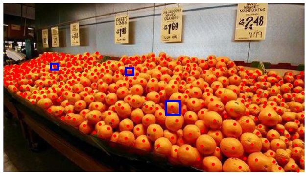
using only the input image and a few exemplars.                  lar the decade-old self-similarity work of Shechtman and
    We propose a novel architecture called Few Shot              Irani [41]. Also related to this idea is the recent work of
Adaptation and Matching Network (FamNet) for tackling            Lu and Zisserman[28], who proposed a Generic Matching
the few-shot counting task. FamNet has two key compo-            Network (GMN) for class-agnostic counting. GMN was
nents: 1) a feature extraction module, and 2) a density pre-     pre-trained with tracking video data, and it had an explicit
diction module. The feature extraction module consists of        adaptation module to adapt the network to an image domain
a general feature extractor capable of handling a large num-     of interest. GMN has been shown to work well if several
ber of visual categories. The density prediction module          dozens to hundreds of examples are available for adapta-
is designed to be agnostic to the visual category. As will       tion. Without adaptation, GMN does not perform very well
be seen in our experiments, both the feature extractor and       on novel classes, as will be seen in our experiments.
density prediction modules can already generalize to the             Related to few-shot counting is the few-shot detection
novel categories at test time. We further improve the per-       task (e.g., [8, 17]), where the objective is to learn a detector
formance of FamNet by developing a novel few-shot adap-          for a novel category using a few labeled examples. Few-
tation scheme at test time. This adaptation scheme uses the      shot counting differs from few-shot detection in two pri-
provided exemplars themselves and adapts the counting net-       mary aspects. First, few-shot counting requires dot anno-
work to them with a few gradient descent updates, where the      tations while detection requires bounding box annotations.
gradients are computed based on two loss functions which         Second, few-shot detection methods can be affected by se-
are designed to utilize the locations of the exemplars to the    vere occlusion whereas few-shot counting is tackled with
fullest extent. Empirically, this adaptation scheme improves     a density estimation approach [22, 55], which is more ro-
the performance of FamNet.                                       bust towards occlusion than the detection-then-counting ap-
    Finally, to address the lack of a dataset for develop-       proach because the density estimation methods do not have
ing and evaluating the performance of few-shot counting          to commit to binarized decisions at an early stage. The ben-
methods, we introduce a medium-scale dataset consisting          efits of the density estimation approach has been empiri-
of more than 6000 images from 147 visual categories. The         cally demonstrated in several domains, especially for crowd
dataset comes with dot and bounding box annotations, and         and cell counting.
is suitable for the few-shot counting task. We name this             Also related to our work is the task of few-shot image
dataset Few-Shot Counting-147 (FSC-147).                         classification [9, 19, 21, 35, 40, 46]. The few-shot classifi-
    In short, the main contributions of our work are as fol-     cation task deals with classifying images from novel cate-
lows. First, we pose counting as a few-shot regression task.     gories at test time, given a few training examples from these
Second, we propose a novel architecture called FamNet for        novel test categories. The Model Agnostic Meta Learning
handling the few-shot counting task, with a novel few-shot       (MAML) [9] based few-shot approach is relevant for our
adaptation scheme at test time. Third, we present a novel        few-shot counting task, and it focuses on learning parame-
few-shot counting dataset called FSC-147, comprising of          ters which can adapt to novel classes at test time by means
over 6000 images with 147 visual categories.                     of few gradient descent steps. However, MAML involves
                                                                 computing second order derivatives during training which
2. Related Works                                                 makes it expensive, even more so for the pixel level predic-
                                                                 tion task of density map prediction being considered in our
   In this work, we are interested in counting objects of in-    paper. Drawing inspiration from these works, we propose a
terest in a given image with a few labeled examples from         novel adaptation scheme which utilizes the exemplars avail-
the same image. Most of the previous counting methods            able at test time and performs a few steps of gradient de-
are for specific types of objects such as people [2, 5, 6, 23,   scent in order to adapt FamNet to any novel category. Un-
26, 27, 29, 32–34, 39, 42, 47, 50, 54, 55], cars [30], an-       like MAML, our training scheme does not require higher
imals [4], cells [3, 18, 53], and fruits [31]. These meth-       order gradients at training time. We compare our approach
ods often require training images with tens of thousands or      with MAML, and empirically show that it leads to better
even millions of annotated object instances. Some of these       performance and is also much faster to train.
works [34] tackle the issue of costly annotation cost to some
extent by adapting a counting network trained on a source        3. Few-Shot Adaptation & Matching Network
domain to any target domain using labels for only few in-
formative samples from the target domain. However, even             In this section, we describe the proposed FamNet for
these approaches require a large amount of labeled data in       tackling the few-shot counting task.
the source domain.
                                                                 3.1. Network architecture
   The proposed FamNet works by exploiting the strong
similarity between a query image and the provided ex-               Fig. 2 depicts the pipeline of FamNet. The input to the
emplar objects in the image. To some extent, it is simi-         network is an image X ∈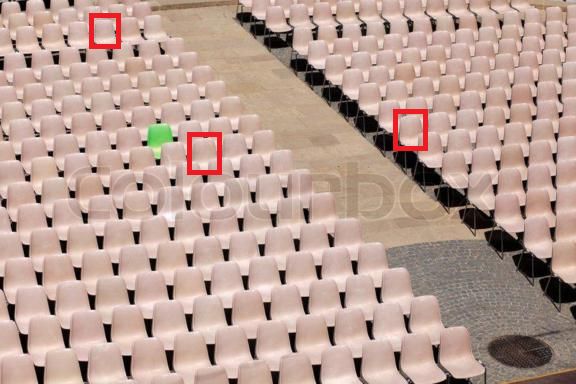
Figure 2: Few-shot adaptation & matching Network takes as input the query image along with few bounding boxes
depicting the object of interest, and predicts the density map. The count is obtained by summing all the pixel values in the
density map. The adaptation loss is computed based on the bounding box information, and the gradients from this loss are
used to update the parameters of the density prediction module. The adaptation loss is only used during test time.

bounding boxes depicting the object to be counted from the       sity map. The size of the predicted density map is the same
same image. The output of the network is the predicted           as the size of the input image.
density map Z ∈
3.3. Test-time adaptation                                        perturbation loss as follows:
                                                                                          X
   Since the two modules of the FamNet are not dependent                        LP er =      ||Zb − Gh×w ||22 .            (2)
on any object categories, the trained FamNet can already be                              b∈B
used for counting objects from novel categories given a few
exemplars. In this section, we describe a novel approach to      The combined adaptation Loss. The loss used for test-
adapt this network to the exemplars, further improving the       time adaptation is the weighted combination of the Min-
accuracy of the estimated count. The key idea is to harness      Count loss and the Perturbation loss. The final test time
the information provided by the locations of the exemplar        adaptation loss is given as
bounding boxes. So far, we have only used the bounding
boxes of the exemplars to extract appearance features of the                LAdapt = λ1 LM inCount + λ2 LP er ,            (3)
exemplars, and we have not utilized their locations to the       where λ1 and λ2 are scalar hyper parameters. At test time,
full extent.                                                     we perform 100 gradient descent steps for each test image,
   Let B denote the set of provided exemplar bounding            and optimize the joint loss presented in Eq. (3). We use the
boxes. For a bounding box b ∈ B, let Zb be the crop from         learning rate 10−7 . The values for λ1 and λ2 are 10−9 and
the density map Z at location b. To harness the extra infor-     10−4 respectively. The learning rate, the number of gradi-
mation provided by the locations of the bounding boxes B,        ent steps, λ1 , and λ2 , are tuned based on the performance on
we propose to consider the following two losses.                 the validation set. The values of λ1 , and λ2 seem small, but
Min-Count Loss. For each exemplar bounding box b, the            this is necessary to make the adaptation loss to have similar
sum of the density values within Zb should be at least one.      magnitude to the training loss. Even though the training loss
This is because the predicted count is taken as the sum of       is not used for test time adaptation, it is important for the
predicted density values, and there is at least one object at    losses and their gradients to have similar magnitudes. Oth-
the location specified by the bounding box b. However, we        erwise, the gradient update steps of the adaptation process
cannot assert that the sum of the density values within Zb to    will either do nothing or move away far from the parameters
be exactly one, due to possible overlapping between b and        learned during training.
other nearby objects of interest. This observation leads to         Note that the adaptation loss is only used at test time.
an inequality constraint: ||Zb ||1 ≥ 1, where ||Zb ||1 denotes   During training of FamNet, this loss is redundant because
the sum of all the values in Zb . Given the predicted density    the proposed training loss, based on mean squared errors
map and the set of provided bounding boxes for the exem-         computed over all pixel locations, already provides stronger
plars, we define the following Min-Count loss to quantify        supervision signal than the adaptation loss.
the amount of constraint violation:
                                                                 4. The FSC-147 Dataset
                         X                                          To train the FamNet, we need a dataset suitable for
          LM inCount =         max(0, 1 − ||Zb ||1 ).     (1)
                                                                 the few-shot counting task, consisting of many visual cate-
                         b∈B
                                                                 gories. Unfortunately, existing counting datasets are mostly
                                                                 dedicated for specific object categories such as people, cars,
Perturbation Loss. Our second loss to harness the po-            and cells. Meanwhile, existing multi-class datasets do not
sitional information provided by the exemplar bounding           contain many images that are suitable for visual count-
boxes is inspired by the success of tracking algorithms          ing. For example, although some images from the COCO
based on correlation filter [13, 44, 51]. Given the bound-       dataset [25] contains multiple instances from the same ob-
ing box of an object to track, these algorithms learn a filter   ject category, most of the images do not satisfy the condi-
that has highest response at the exact location of the bound-    tions of our intended applications due to the small number
ing box and lower responses at perturbed locations. The          of object instances or the huge variation in pose and appear-
correlation filter can be learned by optimizing a regression     ance of the object instances in each image.
function to map from a perturbed location to a target re-           Since there was no dataset that was large and diverse
sponse value, where the target response value decreases ex-      enough for our purpose, we collected and annotated images
ponentially as the perturbation distance increases, usually      ourselves. Our dataset consists of 6135 images across a di-
specified by a Gaussian distribution.                            verse set of 147 object categories, from kitchen utensils and
    In our case, the predicted density map Z is essentially      office stationery to vehicles and animals. The object count
the correlation response map between the exemplars and the       in our dataset varies widely, from 7 to 3731 objects, with
image. To this end, the density values around the location of    an average count of 56 objects per image. In each image,
an exemplar should ideally look like a Gaussian. Let Gh×w        each object instance is annotated with a dot at its approxi-
be the 2D Gaussian window of size h×w. We define the             mate center. In addition, three object instances are selected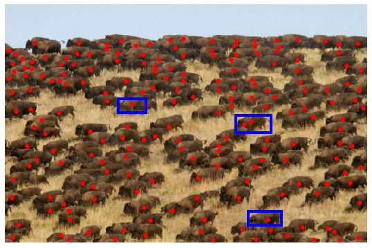
Skat
Apples, 221
2000
169
Alcoh
Cars
Bott
157
eboa
Cans, les, 70
ri es,
ol Bo
le C
, 48
g s,
wber
56
48
rd, 10
tt
Win
aps,
,1
1750
Stra
Vehic
k en
es
122 55
(260) , Box & Ba
to
,1
Chic
Bottle (341)
ma
Vehic
es 39
le le
ap s, 1
To
Pe Gr oll Annotation type
To
n
dR 1500
y
B o cils, 03
(115)
Number of Images
& 349
a
oks 58
Br
e s, 1
Co )
e
Pen , 76
d & Orancuits, 7571
g
(
lle
S ta
Foo uit
s, 9
Dataset Images Categories Dot Bounding Box
cti
g
1 tio
Bis toes,
b
(37 nery
1250
le
4)
Fr 8) Pota , 68
Peas
G reengs, 63
4
Utensil
(20 Eg
Macarons …
, 58 UCF CC 50 [15] 50 1 3 7
Cupcake…
(378) Coffee
Pills, 55
Kidney Beans, 54
1000 Shanghaitech [55] 1198 1 3 7
nts Nuts, 53
eleme
Buildingardware
&H UCF QNRF [16] 1535 1 3 7
ws, 48
Windo s, 58
B rick ds, 71
(398)
750
i B li
n NWPU [49] 5109 1 3 7
&H meti l,
Min irs, 72
(10 ome cs
e
Cha
r
Peo imal
500 JHU Crowd [43] 4372 1 3 3
61 C ppa
Ge
An 81)
ple
es
(10
les 66 3 A
)
s
e,
48
44
s, 4 5 3 CARPK [14] 1448 1 3 3
o
2
&
oe s, , 5 16
S h arl ots
Cr
ck , 6
Pe a D
250
an ns, 1
sti es
Pig ingos
lk
Proposed 6135 147 3 3
s
e
Po
,
Li p gl as
Fla
s,
e
,1
o
m
n
14
23
Su
Bir d
Seag s, 68
5
Crow
s, 4
nd
0
09
ull s,
s, 8
, 10
Ca
1-10 10-20 20-50 50-100 100-300 >300
Bead
7
2
78
Number of objects in an Image (c) Comparison with popular counting datasets.
(a) Image categories and number of im- (b) Number of images in several ranges of
ages for each category in our dataset. object count.
Figure 3: Categories & no. of images per category, object counts, and comparison with other counting datasets
randomly as exemplar instances; these exemplars are also 4. No severe occlusion: in most cases, we removed can-
annotated with axis-aligned bounding boxes. In the follow- didate images where severe occlusion prevents humans
ing subsections, we will describe how the data was collected from accurately counting the objects.
and annotated. We will also report the detailed statistics and
how the data was split into disjoint training, validation, and 4.2. Image Annotation
testing sets. Images in the dataset were annotated by a group of an-
notators using the OpenCV Image and Video Annotation
4.1. Image Collection Tool [1]. Two types of annotation were collected for each
To obtain the set of 6135 images for our dataset, we image, dots and bounding boxes, as illustrated in Fig. 4.
started with a set of candidate images obtained by keyword For images containing multiple categories, we picked only
searches. Subsequently, we performed manual inspection one of the categories. Each object instance in an image
to filter out images that do not satisfy our predefined condi- was marked with a dot at its approximate center. In case
tions as described below. of occlusion, the occluded instance was only counted and
annotated if the amount of occlusion was less than 90%.
Image retrieval. We started with a list of object cate-
For each image, we arbitrarily chose three objects as exem-
gories, and collected 300–3000 candidate images for each
plar instances and we drew axis-aligned bounding boxes for
category by scraping the web. We used Flickr, Google,
those instances.
and Bing search engines with the open source image scrap-
pers [7, 45]. We added adjectives such as many, multiple, 4.3. Dataset split
lots of, and stack of in front of the category names to create
the search query keywords. We divided the dataset into train, validation, and test sets
such that they do not share any object category. We ran-
Manual verification and filtering. We manually inspected domly selected 89 object categories for the train set, and 29
the candidate images and only kept the suitable ones satis- categories each for the validation and test sets. The train,
fying the following criteria: validation, and test sets consist of 3659, 1286 and 1190 im-
ages respectively.
1. High image quality: The resolution should be high
enough to easily differentiate between objects. 4.4. Data Statistics
2. Large enough object count: The number of objects of The dataset contains a total of 6135 images. The aver-
interest should be at least 7. We are more interested in age height and width of the images are 774 and 938 pix-
counting a large number of objects, since humans do els, respectively. The average number of objects per im-
not need help counting a small number of objects. age is 56, and the total number of objects is 343,818. The
3. Appearance similarity: we selected images where ob- minimum and maximum number of objects for one image
ject instances have somewhat similar poses, texture, are 7 and 3701, respectively. The three categories with the
and appearance. highest number of objects per image are: Lego (303 ob-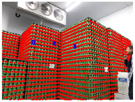
Val-COCO Set Test-COCO Set
                                   Val Set        Test Set
                                                                    Method                MAE RMSE MAE RMSE
 Method                        MAE RMSE MAE RMSE
                                                                    Faster R-CNN          52.79   172.46   36.20    79.59
 Mean                          53.38   124.53   47.55   147.67      RetinaNet             63.57   174.36   52.67    85.86
 Median                        48.68   129.70   47.73   152.46      Mask R-CNN            52.51   172.21   35.56    80.00
 FR few-shot detector [17]     45.45   112.53   41.64   141.04      FamNet (Proposed)     39.82   108.13   22.76    45.92
 FSOD few-shot detector [8]    36.36   115.00   32.53   140.65
 Pre-trained GMN [28]          60.56   137.78   62.69   159.67   Table 2: Comparing FamNet with pre-trained object de-
 GMN [28]                      29.66    89.81   26.52   124.57   tectors, on counting objects from categories where there are
 MAML [9]                      25.54    79.44   24.90   112.68   pre-trained object detectors.
 FamNet (Proposed)             23.75   69.07    22.08   99.54
                                                                 meta parameters that facilitate faster generalization to novel
Table 1: Comparing FamNet to two simple baselines                tasks. At test time, only the inner optimization is performed.
(Mean, Median) and four stronger baseline (Feature               We use the LAdapt loss defined in Eq. (3) for the inner op-
Reweighting (FR) few-shot detector, FSOD few-shot de-            timization loop, and the MSE loss over the entire dot anno-
tector, GMN and MAML), these are few-shot methods that           tation map for the outer optimization loop.
have been adapted and trained for counting. FamNet has the           As can be seen in Table 1, FamNet outperforms all the
lowest MAE and RMSE on both val and test sets.                   other methods. Surprisingly, the pre-trained GMN does not
                                                                 work very well, even though it is a class agnostic count-
jects/image), Brick (271), and Marker (247). The three cat-
                                                                 ing method. The GMN model trained on our training data
egories with lowest number of objects per image are: Su-
                                                                 performs better than its pre-trained version; and this demon-
permarket shelf (8 objects/image), Meat Skewer (8), and
                                                                 strates the benefits of our dataset. The state-of-the-art few-
Oyster (11). Fig. 3b is a histogram plot for the number of
                                                                 shot detectors [8, 17] perform relatively poor, even when
images in several ranges of object count.
                                                                 they are trained on our dataset. With these results, we are
                                                                 the first to show the empirical evidence for the inferiority
5. Experiments                                                   of the detection-then-counting approach compared to the
5.1. Performance Evaluation Metrics                              density estimation approach (GMN, MAML, FamNet) for
                                                                 generic object counting. However, this is not new for the
    We use Mean Absolute Error (MAE) and Root Mean               crowd counting research community, where the density esti-
Squared Error (RMSE) to measure the accuracy of a count-         mation approach dominates the recent literature [55], thanks
ing method. MAE and RMSE are commonly used met-                  to its robustness to occlusion and the freedom of not having
rics for counting task [29, 32,    Pn55], and they are de-       to commit to binarized decisions at an early stage. Among
fined as follows. M AE = n1 i=1 |ci − ĉi |; RM SE =             the competing approaches, MAML is the best method of all.
q P
   1   n              2
   n   i=1 (ci − ĉi ) , where n is the number of test images,   This is perhaps because MAML is a meta learning method
and ci and ĉi are the ground truth and predicted counts.        that leverages the advantages of having the FamNet archi-
                                                                 tecture as its core component. The MAML way of training
5.2. Comparison with Few-Shot Approaches                         this network leads to a better model than GMN, but it is
    We compare the performance of FamNet with two triv-          still inferior to the proposed FamNet together with the pro-
ial baselines and four competing few-shot methods. The           posed training and adaptation algorithms. In terms of train-
two trivial baseline methods are: (1) always output the av-      ing time per epoch, FamNet is around three times faster than
erage object count for training images; (2) always output        MAML, because it does not require any higher order gradi-
the median count for the training images. We also imple-         ent computation like MAML.
ment stronger methods for comparison, by adapting several
                                                                 5.3. Comparison with Object Detectors
few-shot methods for the counting task and training them
on our training data. Specifically, we adapt the following          One approach for counting is to use a detector to de-
approaches for counting: the state-of-the-art few-shot de-       tect objects and then count. This approach only works for
tectors [8, 17], the Generic Matching Network (GMN) [28],        certain categories of objects, where there are detectors for
and Model Agnostic Meta Learning (MAML) [9]. We im-              those categories. In general, it requires thousands of ex-
plement MAML using the higher library [10], which is a           amples to train an object detector, so this is not a practi-
meta learning library supporting higher order optimization.      cal method for general visual counting. Nevertheless, we
The training procedure of MAML involves an inner op-             evaluate the performance of FamNet on a subset of cate-
timization loop, which adapts the network to the specific        gories from the validation and test sets that have pre-trained
test classes, and an outer optimization loop which learns        object detectors on the COCO dataset. We refer to these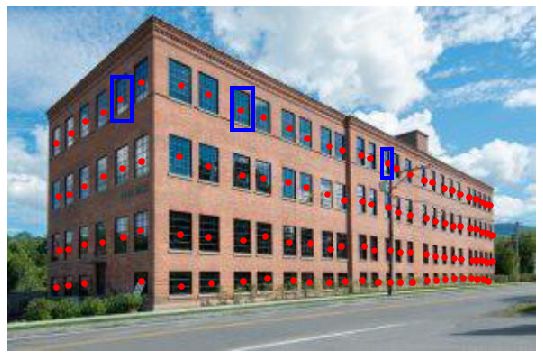
Figure 4: Few annotated images from the dataset. Dot and box annotations are shown in red and blue respectively. The
number of objects in each image varies widely, some images contain a dozen of objects while some contains thousands.

       Number of Exemplars         MAE        RMSE             as the number of exemplars increases, and (2) the benefits
                                                               of different components of FamNet.
                  1               26.55       77.01
                                                                  In Table 3, we analyze the performance of FamNet as the
                  2               24.09       72.37
                                                               number of exemplars is varied between one to three dur-
                  3               23.75       69.07
                                                               ing the testing of FamNet. We see that FamNet can work
Table 3: Performance of FamNet on the validation data as       even with one exemplar, and it outperforms all the com-
the number of exemplars increases. FamNet can provide a        peting methods presented in Table 1 with just 2 exemplars.
reasonable count estimate even with a single exemplar, and     Not surprisingly, the performance of FamNet improves as
the estimate becomes more accurate with more exemplars.        the number of exemplars is increased. This suggests that
                                                               an user of our system can obtain a reasonable count even
subsets as Val-COCO and Test-COCO, which comprise of           with a single exemplar, and they can obtain a more accurate
277 and 282 images respectively. Specifically, we com-         count by providing more exemplars.
pare FamNet with FasterRCNN [37], MaskRCNN [11], and              In Table 4, we analyze the importance of the key compo-
RetinaNet [24]. All of these pretrained detectors are avail-   nents of FamNet: multi-scale image feature map, the multi-
able in the Detectron2 library [52]. Table 2 shows the com-    scale exemplar features, and test time adaptation. We train
parison results. As can be seen, FamNet outperforms the        models without few/all of these components on the train-
pre-trained detectors, even on object categories where the     ing set of FSC-147, and report the validation performance.
detectors have been trained with thousands of annotated ex-    We notice that all of the components of FamNet are impor-
amples from the COCO dataset.                                  tant, and adding each of the component leads to improved
                                                               results.
Components                            Combinations
Multi-scale image feature         7       X     X       X      5.5. Counting category-specific objects
Multi-scale exemplar feature      7       7     X       X         FamNet is specifically designed to be general, being able
Test time adaptation              7       7     7       X      to count generic objects with only a few exemplars. As
MAE                            32.70 27.80 24.32 23.75         such, it might not be fair to demand it to work extremely
RMSE                           104.31 93.53 70.94 69.07        well for a specific category, such as counting cars. Cars are
                                                               popular objects that appear in many datasets and this cat-
Table 4: Analyzing the components of FamNet. Each of
                                                               egory is the explicit or implicit target for tuning for many
the components of FamNet adds to the performance.
                                                               networks, so it would not be surprising if our method does
                                                               not perform as well as other customized solutions. Having
                                                               said that, we still investigate the suitability of using FamNet
5.4. Ablation Studies
                                                               to count cars from the CARPK dataset [14], which consists
  We perform ablation studies on the validation set of FSC-    of overhead images of parking lots taken by downward fac-
147 to analyze: (1) how the counting performance changes       ing drone cameras. The training and test set consists of 989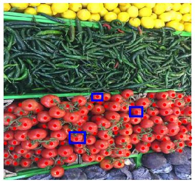
Image                       Prediction
   Method                                     MAE RMSE
   YOLO [14, 36]                              48.89    57.55
   Faster RCNN [14, 38]                       47.45    57.39
   One-look Regression [14, 30]               59.46    66.84
   Faster RCNN [14, 38](RPN-small)            24.32    37.62
   Spatially Regularized RPN [14]             23.80    36.79               GT Count: 263                 Pred Count: 280
   GMN [28]                                    7.48     9.90
   FamNet– (pre-trained)                      28.84    44.47
   FamNet+ (trained with CARPK data)          18.19    33.66
Table 5: Counting car performance on the CARPK
dataset. FamNet– is a FamNet model, that is trained with-
out any CARPK images nor images from the car category
of FSC-147. Other methods use the entire CARPK train                        GT Count: 77                 Pred Count: 77
set. Pre-trained FamNet– outperforms three of of the previ-
ous approaches. FamNet+, yields even better performance.

and 459 images respectively. There are around 90,000 in-
stances of cars in the dataset.
    We experiment with two variants of FamNet: a pre-                       GT Count: 47                 Pred Count: 46
trained model and a model trained on CARPK dataset.
The pre-trained FamNet model is called FamNet–, which is
trained on FSC-147, without using the data from CARPK or
the car category from FSC-147. The FamNet model trained
with training data from CARPK is called FamNet+, and it is
trained as follows. We randomly sample a set of 12 exem-
plars from the training set, and use these as the exemplars                 GT Count: 77                 Pred Count: 192
for all of the training and test images. We train FamNet+
on the CARPK training set. Table 5 displays the results of          Figure 5: Predicted density maps and counts of FamNet.
several methods on this CARPK dataset. FamNet+ outper-                     Image            Pre Adapt.          Post Adapt.
forms all methods except GMN [28]. GMN, unlike all the
other approaches, uses extra training data from the ILSVRC
video dataset which consists of video sequences of cars.
Perhaps this may be why GMN works particularly well on
CARPK.
                                                                      GT Count: 240         Count: 356          Count: 286
5.6. Qualitative Results
                                                                    Figure 6: Test time adaptation. Shown are the initial den-
    Fig. 5 shows few images and FamNet predictions. The             sity map (Pre Adapt) and final density map after adaptation
first three are success cases,and the last is a failure case. For   (Post Adapt). In case of over counting, adaptation decreases
the fourth image, FamNet confuses portions of the back-             the density values at dense locations.
ground as being the foreground, because of similarity in ap-
pearance between the background and the object of interest.         instances. We also presented a novel approach for density
Fig. 6 shows a test case where test time adaptation improves        prediction suitable for the few-shot visual counting task. We
on the initial count by decreasing the density values in the        compared our approach with several state-of-art detectors
dense regions.                                                      and few shot counting approaches, and showed that our ap-
                                                                    proach outperforms all of these approaches.
6. Conclusions
   In this paper, we posed counting as a few-shot regres-           Acknowledgements: This project is partially supported by
sion task. Given the non-existence of a suitable dataset for        MedPod, the SUNY2020 Infrastructure Transportation Se-
the few-shot counting task, we collected a visual counting          curity Center, and the NSF I/UCRC Center for Visual and
dataset with relatively large number of object categories and       Decision Informatics at Stony Brook.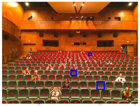
References                                                                 European Conference on Computer Vision, 2018.
                                                                      [17] Bingyi Kang, Zhuang Liu, Xin Wang, Fisher Yu, Jiashi Feng,
 [1] Computer vision annotation tool.                                      and Trevor Darrell. Few-shot object detection via feature
 [2] Shahira Abousamra, Minh Hoai, Dimitris Samaras, and                   reweighting. In Proceedings of the International Conference
     Chao Chen. Localization in the crowd with topological con-            on Computer Vision, 2019.
     straints. In Proceedings of AAAI Conference on Artificial        [18] Aisha Khan, Stephen Gould, and Mathieu Salzmann. Deep
     Intelligence, 2021.                                                   convolutional neural networks for human embryonic cell
 [3] Carlos Arteta, Victor Lempitsky, J Alison Noble, and An-              counting. In Proceedings of the European Conference on
     drew Zisserman. Detecting overlapping instances in mi-                Computer Vision. Springer, 2016.
     croscopy images using extremal region trees. Medical image       [19] Gregory Koch, Richard Zemel, and Ruslan Salakhutdinov.
     analysis, 27:3–16, 2016.                                              Siamese neural networks for one-shot image recognition. In
 [4] Carlos Arteta, Victor Lempitsky, and Andrew Zisserman.                ICML deep learning workshop, 2015.
     Counting in the wild. In Proceedings of the European Con-        [20] Brenden M. Lake, Ruslan Salakhutdinov, and Joshua B.
     ference on Computer Vision, 2016.                                     Tenenbaum. Human-level concept learning through proba-
 [5] Deepak Babu Sam, Neeraj N Sajjan, R Venkatesh Babu, and               bilistic program induction. Science, 350(6266):1332–1338,
     Mukundhan Srinivasan. Divide and grow: Capturing huge                 December 2015.
     diversity in crowd images with incrementally growing cnn.        [21] Brenden M Lake, Ruslan Salakhutdinov, and Joshua B
     In Proceedings of the IEEE Conference on Computer Vision              Tenenbaum. Human-level concept learning through proba-
     and Pattern Recognition, 2018.                                        bilistic program induction. Science, 350(6266):1332–1338,
 [6] Xinkun Cao, Zhipeng Wang, Yanyun Zhao, and Fei Su. Scale              2015.
     aggregation network for accurate and efficient crowd count-      [22] Victor Lempitsky and Andrew Zisserman. Learning to count
     ing. In Proceedings of the European Conference on Com-                objects in images. In Advances in Neural Information Pro-
     puter Vision, 2018.                                                   cessing Systems, 2010.
 [7] Del Riccardo Chiaro. python-flickr-image-downloader.             [23] Yuhong Li, Xiaofan Zhang, and Deming Chen. Csrnet: Di-
 [8] Qi Fan, Wei Zhuo, Chi-Keung Tang, and Yu-Wing Tai. Few-               lated convolutional neural networks for understanding the
     shot object detection with attention-rpn and multi-relation           highly congested scenes. In Proceedings of the IEEE Con-
     detector. In Proceedings of the IEEE Conference on Com-               ference on Computer Vision and Pattern Recognition, 2018.
     puter Vision and Pattern Recognition, 2020.                      [24] Tsung-Yi Lin, Priya Goyal, Ross Girshick, Kaiming He, and
 [9] Chelsea Finn, Pieter Abbeel, and Sergey Levine. Model-                Piotr Dollár. Focal loss for dense object detection. In Pro-
     agnostic meta-learning for fast adaptation of deep networks.          ceedings of the International Conference on Computer Vi-
     In Proceedings of the International Conference on Machine             sion, 2017.
     Learning, 2017.                                                  [25] Tsung-Yi Lin, Michael Maire, Serge Belongie, Lubomir
[10] Edward Grefenstette, Brandon Amos, Denis Yarats,                      Bourdev, Ross Girshick, James Hays, Pietro Perona, Deva
     Phu Mon Htut, Artem Molchanov, Franziska Meier, Douwe                 Ramanan, C. Lawrence Zitnick, and Piotr Dollár. Microsoft
     Kiela, Kyunghyun Cho, and Soumith Chintala. Generalized               COCO: Common objects in context. In Proceedings of the
     inner loop meta-learning. arXiv preprint arXiv:1910.01727,            European Conference on Computer Vision, 2014.
     2019.                                                            [26] Weizhe Liu, Mathieu Salzmann, and Pascal Fua. Context-
[11] Kaiming He, Georgia Gkioxari, Piotr Dollár, and Ross Gir-            aware crowd counting. In Proceedings of the IEEE Confer-
     shick. Mask R-CNN. In Proceedings of the International                ence on Computer Vision and Pattern Recognition, 2019.
     Conference on Computer Vision, 2017.                             [27] Xialei Liu, Joost Van De Weijer, and Andrew D Bagdanov.
[12] Kaiming He, Xiangyu Zhang, Shaoqing Ren, and Jian Sun.                Leveraging unlabeled data for crowd counting by learning to
     Deep residual learning for image recognition. In Proceed-             rank. In Proceedings of the IEEE Conference on Computer
     ings of the IEEE Conference on Computer Vision and Pattern            Vision and Pattern Recognition, 2018.
     Recognition, 2016.                                               [28] Erika Lu, Weidi Xie, and Andrew Zisserman. Class-agnostic
[13] J. F. Henriques, R. Caseiro, P. Martins, and J. Batista. High-        counting. In Proceedings of the Asian Conference on Com-
     speed tracking with kernelized correlation filters. IEEE              puter Vision, 2018.
     Transactions on Pattern Analysis and Machine Intelligence,       [29] Zhiheng Ma, Xing Wei, Xiaopeng Hong, and Yihong Gong.
     37(3):583–596, 2015.                                                  Bayesian loss for crowd count estimation with point super-
[14] Meng-Ru Hsieh, Yen-Liang Lin, and Winston H Hsu. Drone-               vision. In Proceedings of the International Conference on
     based object counting by spatially regularized regional pro-          Computer Vision, 2019.
     posal network. In Proceedings of the International Confer-       [30] T Nathan Mundhenk, Goran Konjevod, Wesam A Sakla, and
     ence on Computer Vision, 2017.                                        Kofi Boakye. A large contextual dataset for classification,
[15] Haroon Idrees, Imran Saleemi, Cody Seibert, and Mubarak               detection and counting of cars with deep learning. In Pro-
     Shah. Multi-source multi-scale counting in extremely dense            ceedings of the European Conference on Computer Vision,
     crowd images. In Proceedings of the IEEE Conference on                2016.
     Computer Vision and Pattern Recognition, 2013.                   [31] Maryam Rahnemoonfar and Clay Sheppard. Deep count:
[16] Haroon Idrees, Muhmmad Tayyab, Kishan Athrey, Dong                    fruit counting based on deep simulated learning. Sensors,
     Zhang, Somaya Al-Maadeed, Nasir Rajpoot, and Mubarak                  17(4):905, 2017.
     Shah. Composition loss for counting, density map estima-         [32] Viresh Ranjan, Hieu Le, and Minh Hoai. Iterative crowd
     tion and localization in dense crowds. In Proceedings of the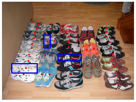
counting. In Proceedings of the European Conference on                  crowd: A large-scale benchmark for crowd counting. arXiv
       Computer Vision, 2018.                                                  preprint arXiv:2001.03360, 2020.
[33]   Viresh Ranjan, Mubarak Shah, and Minh Hoai                       [50]   Qi Wang, Junyu Gao, Wei Lin, and Yuan Yuan. Learning
       Nguyen. Crowd transformer network. arXiv preprint                       from synthetic data for crowd counting in the wild. In Pro-
       arXiv:1904.02774, 2019.                                                 ceedings of the IEEE Conference on Computer Vision and
[34]   Viresh Ranjan, Boyu Wang, Mubarak Shah, and Minh                        Pattern Recognition, 2019.
       Hoai. Uncertainty estimation and sample selection for crowd      [51]   Qiang Wang, Li Zhang, Luca Bertinetto, Weiming Hu, and
       counting. In Proceedings of the Asian Conference on Com-                Philip HS Torr. Fast online object tracking and segmentation:
       puter Vision, 2020.                                                     A unifying approach. In Proceedings of the IEEE Conference
[35]   Sachin Ravi and Hugo Larochelle. Optimization as a model                on Computer Vision and Pattern Recognition, 2019.
       for few-shot learning. 2016.                                     [52]   Yuxin Wu, Alexander Kirillov, Francisco Massa, Wan-Yen
[36]   Joseph Redmon, Santosh Divvala, Ross Girshick, and Ali                  Lo, and Ross Girshick. Detectron2, 2019.
       Farhadi. You only look once: Unified, real-time object de-       [53]   Weidi Xie, J Alison Noble, and Andrew Zisserman. Mi-
       tection. In Proceedings of the IEEE Conference on Computer              croscopy cell counting and detection with fully convolu-
       Vision and Pattern Recognition, 2016.                                   tional regression networks. Computer methods in biome-
[37]   Shaoqing Ren, Kaiming He, Ross Girshick, and Jian Sun.                  chanics and biomedical engineering: Imaging & Visualiza-
       Faster R-CNN: Towards real-time object detection with re-               tion, 6(3):283–292, 2018.
       gion proposal networks. In Advances in Neural Information        [54]   Anran Zhang, Lei Yue, Jiayi Shen, Fan Zhu, Xiantong Zhen,
       Processing Systems. 2015.                                               Xianbin Cao, and Ling Shao. Attentional neural fields for
[38]   Shaoqing Ren, Kaiming He, Ross Girshick, and Jian Sun.                  crowd counting. In Proceedings of the International Confer-
       Faster r-cnn: Towards real-time object detection with region            ence on Computer Vision, 2019.
       proposal networks. In Advances in Neural Information Pro-        [55]   Yingying Zhang, Desen Zhou, Siqin Chen, Shenghua Gao,
       cessing Systems, 2015.                                                  and Yi Ma. Single-image crowd counting via multi-column
[39]   Deepak Babu Sam, Shiv Surya, and R Venkatesh Babu.                      convolutional neural network. In Proceedings of the IEEE
       Switching convolutional neural network for crowd counting.              Conference on Computer Vision and Pattern Recognition,
       In Proceedings of the IEEE Conference on Computer Vision                2016.
       and Pattern Recognition, 2017.
[40]   Adam Santoro, Sergey Bartunov, Matthew Botvinick, Daan
       Wierstra, and Timothy Lillicrap. One-shot learning with
       memory-augmented neural networks. 2016.
[41]   Eli Shechtman and Michal Irani. Matching local self-
       similarities across images and videos. In Proceedings of the
       IEEE Conference on Computer Vision and Pattern Recogni-
       tion, 2007.
[42]   Miaojing Shi, Zhaohui Yang, Chao Xu, and Qijun Chen. Re-
       visiting perspective information for efficient crowd counting.
       In Proceedings of the IEEE Conference on Computer Vision
       and Pattern Recognition, 2019.
[43]   Vishwanath A Sindagi, Rajeev Yasarla, and Vishal M Pa-
       tel. Jhu-crowd++: Large-scale crowd counting dataset and
       a benchmark method. arXiv preprint arXiv:2004.03597,
       2020.
[44]   Jack Valmadre, Luca Bertinetto, Joao Henriques, Andrea
       Vedaldi, and Philip HS Torr. End-to-end representation
       learning for correlation filter based tracking. In Proceed-
       ings of the IEEE Conference on Computer Vision and Pattern
       Recognition, 2017.
[45]   Hardik Vasa. Google images download.
[46]   Oriol Vinyals, Charles Blundell, Timothy Lillicrap, Daan
       Wierstra, et al. Matching networks for one shot learning. In
       Advances in Neural Information Processing Systems, 2016.
[47]   Jia Wan and Antoni Chan. Adaptive density map genera-
       tion for crowd counting. In Proceedings of the IEEE Inter-
       national Conference on Computer Vision, pages 1130–1139,
       2019.
[48]   Boyu Wang, Huidong Liu, Dimitris Samaras, and Minh
       Hoai. Distribution matching for crowd counting. In Ad-
       vances in Neural Information Processing Systems. 2020.
[49]   Qi Wang, Junyu Gao, Wei Lin, and Xuelong Li. Nwpu-
You can also read