MAGNETOTELLURIC SIGNAL-NOISE IDENTIFICATION AND SEPARATION BASED ON APEN-MSE AND STOMP - MDPI
←
→
Page content transcription
If your browser does not render page correctly, please read the page content below
entropy
Article
Magnetotelluric Signal-Noise Identification and
Separation Based on ApEn-MSE and StOMP
Jin Li 1, *, Jin Cai 1 , Yiqun Peng 1 , Xian Zhang 1 , Cong Zhou 2 , Guang Li 2, * and Jingtian Tang 3
 1   Hunan Provincial Key Laboratory of Intelligent Computing and Language Information Processing,
     College of Information Science and Engineering, Hunan Normal University, Changsha 410081, China;
     13723863403@163.com (J.C.); yqunpeng@163.com (Y.P.); zxian128@163.com (X.Z.)
 2   State Key Laboratory of Nuclear Resources and Environment, East China University of Technology,
     Nanchang 330013, China; zhoucong_522@163.com
 3   School of Geosciences and Info-Physics, Central South University, Changsha 410083, China;
     jttang@csu.edu.cn
 *   Correspondence: geologylj@163.com (J.L.); li_guangg@163.com (G.L.); Tel.: +86-731-8887-2192 (J.L. & G.L.)

 Received: 15 December 2018; Accepted: 13 February 2019; Published: 19 February 2019

 Abstract: Natural magnetotelluric signals are extremely weak and susceptible to various types
 of noise pollution. To obtain more useful magnetotelluric data for further analysis and research,
 effective signal-noise identification and separation is critical. To this end, we propose a novel
 method of magnetotelluric signal-noise identification and separation based on ApEn-MSE and
 Stagewise orthogonal matching pursuit (StOMP). Parameters with good irregularity metrics are
 introduced: Approximate entropy (ApEn) and multiscale entropy (MSE), in combination with
 k-means clustering, can be used to accurately identify the data segments that are disturbed by noise.
 Stagewise orthogonal matching pursuit (StOMP) is used for noise suppression only in data segments
 identified as containing strong interference. Finally, we reconstructed the signal. The results show
 that the proposed method can better preserve the low-frequency slow-change information of the
 magnetotelluric signal compared with just using StOMP, thus avoiding the loss of useful information
 due to over-processing, while producing a smoother and more continuous apparent resistivity curve.
 Moreover, the results more accurately reflect the inherent electrical structure information of the
 measured site itself.

 Keywords: magnetotelluric; signal-noise identification and separation; approximate entropy (ApEn);
 multiscale entropy (MSE); stagewise orthogonal matching pursuit (StOMP)

1. Introduction
     Since the Soviet scholar, Tikhonov, and the French scholar, Cagniard, proposed the magnetotelluric
(MT) method in the early 1950s [1,2], with its unique advantages, it has gradually been regarded by
geophysicists as an important and indispensable method for geophysical exploration. As it is a kind
of electrical branch method for sounding by changing the frequency of the electromagnetic field,
the exploration depth varies with the frequency of the electromagnetic field. The shallowest depths
can be tens of meters while the deepest depths can be up to hundreds of kilometers. It has been widely
used in many fields, such as the survey and exploration of petroleum and natural gas, the investigation
of geothermal fields, and the prediction of natural earthquakes, etc. [3–6]. In addition, it is used to
study the electrical structure of the crust and upper mantle, in which the discovery of the highly
conductive layer provides an important basis for tectonic mechanics.
     A direct problem faced is that natural magnetotelluric signals are extremely weak and are
susceptible to various types of noise pollution. Performing effective signal-noise identification and the

Entropy 2019, 21, 197; doi:10.3390/e21020197                                    www.mdpi.com/journal/entropy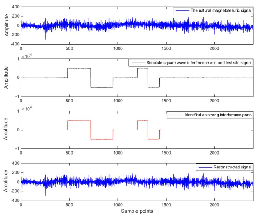
Entropy 2019, 21, 197                                                                                            2 of 15

separation of magnetotelluric signals [7,8] has always been a challenge. However, the effectiveness of
processing directly affects further analysis of magnetotelluric signals. So far, there have been many
methods for the processing of magnetotelluric signals. Most of them are overall processing and, as they
lack signal-noise identification, they can easily cause the over-processing of signals and a loss of
useful information. Taking this into account, this paper introduces the k-means clustering algorithm,
approximate entropy (ApEn), and multiscale entropy (MSE) as the signal-noise identification method.
      The k-means clustering algorithm [9–11] is a hard clustering algorithm, which is representative
of a typical prototype-based clustering method for objective functions. It utilizes the distance from
data points to the prototype as an optimized objective function and an adjustment rule of iterative
operation is obtained by using the method of function extreme value evaluation [12–15]. Entropy is
a method of measuring and quantitatively describing the randomness or irregularity of a time series
or nonlinear signals [16]. Pincus first proposed the ApEn method in 1991 [17], and Richman and
Moorman then proposed the sample entropy (SampEn) [18]; both have the advantages of minimal
data requirements, strong anti-noise ability, etc. However, SampEn is a measure of the irregularity
of a time series on a single scale, whereas Costa et al. developed another method, MSE, based on
the sample entropy [19,20]; it is used to measure the irregularity of time series at different scales and
greatly enhances the applicability of entropy [21–23]. The above values of entropy can be used as
indicators and characteristic parameters to characterize the randomness or irregularity of different
types of signals [24,25]. This paper will demonstrate how ApEn and MSE, in combination with k-means
clustering, can be used to accurately identify weak magnetotelluric signals and noise interference.
Based on ensuring the accuracy of signal-noise identification, the loss of useful information is
avoided. In recent years, Donoho et al. proposed a new theory of information acquisition known as
compressed sensing [26,27]. Compressed sensing theory mainly includes the sparse representation of
signals, an observation matrix measurement, and a reconstruction algorithm. Stagewise orthogonal
matching pursuit (StOMP) belongs to the class of greedy reconstruction algorithms in compressed
sensing theory [28,29]. It is an improved algorithm for matching pursuit (MP) [30,31] as well as
orthogonal matching pursuit (OMP) [32,33]. Compared with MP and OMP, it can further improve the
computational efficiency, reduce the computational cost, and improve the de-noising performance.
Thus, we propose a novel method of magnetotelluric signal-noise identification and separation based
on ApEn-MSE and StOMP.
      Although ApEn-MSE does not seem to be directly related to StOMP, they are two indispensable
components of the magnetotelluric signal-noise identification and separation method. ApEn-MSE is
used as part of the magnetotelluric signal-noise identification, and StOMP is used for the magnetotelluric
signal-noise separation. Without the previous signal-noise identification, the subsequent signal-noise
separation will have no target.

2. Methods

2.1. Approximate Entropy (ApEn)
     ApEn is a measuring method that quantitatively describes the irregularity of nonlinear signals [34–37].
Taking the time series {u(i )/i = 1, 2, · · · , N } of length N as an example, the regularity of u(i ) can
be measured by approximate entropy in a multi-dimensional space. The approximate entropy is
calculated as follows:
     (1) Reconstruct the m-dimensional vector, R(i ), according to the sequence, {u(i )}:

                        R(i ) = (u(i ), u(i + 1), · · · , u(i + m − 1)), i = 1, 2, · · · , N − m + 1                (1)

      (2) Calculate the distance, d( R(i ), R( j)), between the elements of vector R(i ) and R( j):

                 d( R(i ), R( j)) =       max           {|u(i + k) − u( j + k)|}i, j = 1, 2, · · · , N − m + 1      (2)
                                      k =0,1,··· ,m−1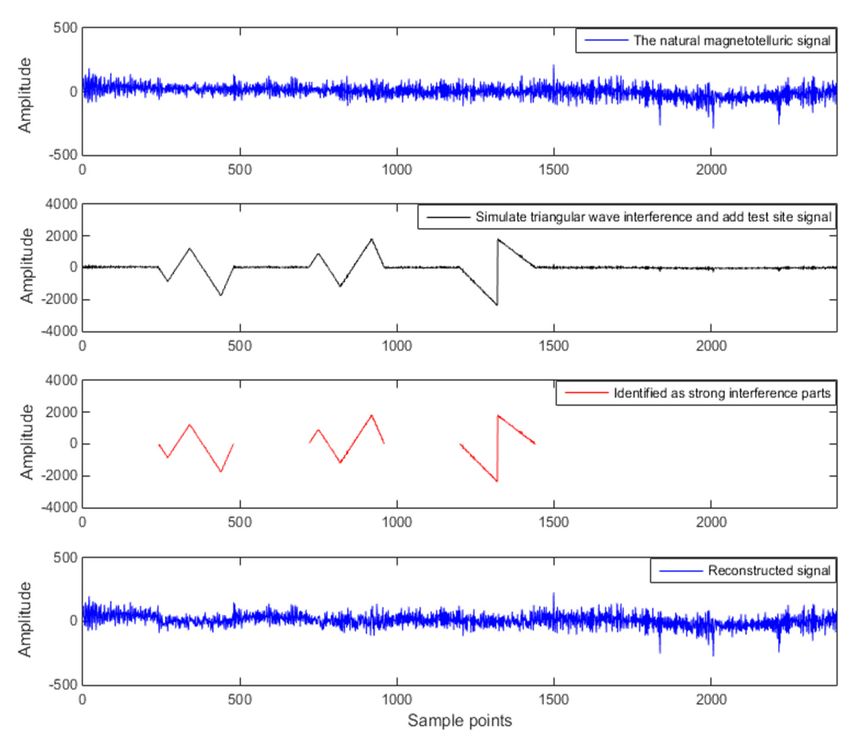
Entropy 2019, 21, 197                                                                                3 of 15

     (3) For each i value and a measure of similarity, λ(λ > 0), the number of vectors, R( j), satisfying
the condition, d( R(i ), R( j)) < λ, is calculated. Additionally, the ratio of this number with respect to
the total N − m + 1 is called Cim (λ):

                                         number       o f {d( R(i ), R( j)) < λ}
                             Cim (λ) =                                                                  (3)
                                                       N−m+1

      (4) The similarity, Cim (λ), in the above formula is taken as a logarithm, and the average value of i
                               1      N − m +1
is obtained: Φm (λ) =                    ∑ ln Cim (λ); by increasing the dimension to m + 1 and repeating
                         N − m + 1 i =1
the above step (1) through to (3), Φm+1 (λ) is obtained. The approximate entropy of the time series,
{u(i )}, is defined as:
                                     ApEn(m, λ, N ) = Φm (λ) − Φm+1 (λ)                                (4)

      The larger the approximate entropy, the more random or irregular the signal will be.

2.2. Sample Entropy (SampEn)
     SampEn is a time series complexity measure method, which has the advantages of simple
calculation and fast speed [38–41]. The larger the sample entropy, the more random or irregular
the sequence and the lower the self-similarity.
     The calculation steps of the sample entropy of the time series, {u(i )}, with length N are similar to
the approximate entropy in Section 2.1 and are defined as follows:

                                                                      B m +1 ( λ )
                                   SampEn(m, λ, N ) = − ln                                              (5)
                                                                       Bm (λ)

where λ represents a measure of similarity, Bm (λ) represents a logarithmic mean of similarity,
and Bm+1 (λ) represents an m + 1-dimensional, Bm (λ).
      Sample entropy can be used to describe nonlinear signals with a high complexity and a large
computational requirement [42,43].
      In the experiment, the embedding dimension, m, of the approximate entropy and the sample
entropy is taken as 2, while the similarity tolerance, λ, of the approximate entropy and sample entropy
is 0.25 times the standard deviation.

2.3. Multiscale Entropy (MSE)
     MSE is used to calculate the sample entropy on multiple scales of the original signal and it is
obtained by using a coarse granulation process at different scales [44–47].
     (1) Take nthe one-dimensional
                    o              time series, {u(i )/i = 1, 2, · · · , N }, as an example. A new coarse
grain vector, y(τ ) , could be obtained as follows:

                                                               jτ
                                                              ∑
                                           (τ )
                                         yj       = 1/τ                   ui                            (6)
                                                          i =( j−1)τ +1

where 1 ≤ j ≤ N/τ, and the scaling factor, τ, is an integer in the [1, 2, · · · , τmax ].
     (2) The sample entropy of τ coarse-grained sequences is also obtained. The MSE analysis is
calculated by plotting MSE as a function of the scaling factor, τ.

2.4. Stagewise Orthogonal Matching Pursuit (StOMP)
     Suppose x is a discrete signal of length N, in the sparse base, Ψ = [ψ1 , ψ2 , · · · ψN ], only K
coefficients are not 0 or significantly larger than other coefficients, and K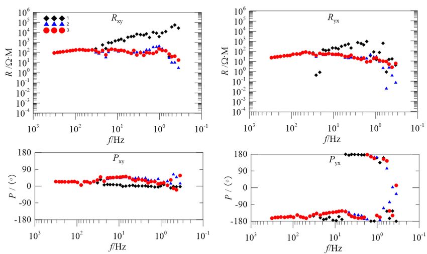
Entropy 2019, 21, 197                                                                                    4 of 15

                                                     N
the sparse basis, Ψ = [ψ1 , ψ2 , · · · ψN ], then x = ∑ Si ψi = ΨS. M(K  10 or krs k2 < OPT × kyk2 (OPT = 10−6 ), the algorithm
                        ∧
terminates and xs = xs is the final output. Otherwise, set s = s + 1 and we proceed to the above
step (2) to continue with the algorithm flow.

3. Simulation Analysis

3.1. Sample Library Signals Classification
     Figure 1 is two 3D clustering effect diagrams of sample library signals [49]. The x-axis represents
the number of samples. The y-axis represents the characteristic parameter values calculated for
200 samples. The z-axis indicates that the two different types are formed by extracting the characteristic
parameters from the sample library signals as input to the k-means clustering. The first 50 are without
electromagnetic interference samples, and the other 150 are samples that are subject to three types of
interference (square wave interference, triangular interference, and pulse interference).
     Since the time series of the sample library signals without electromagnetic interference are more
random and irregular, as shown in Figure 1, the characteristic parameter value (ApEn or MSE) of MT
signals without electromagnetic interference is significantly higher than that of the sample library
signals with interference. Moreover, the greater the calculated entropy value, the less interference the
signal is subjected to. Therefore, it is feasible to calculate the entropy of the MT signal and input it to
the k-means clustering to obtain two different types of signals to realize signal-noise identification.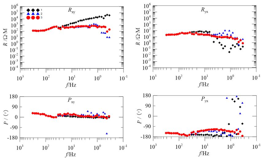
Since the time series of the sample library signals without electromagnetic interference are more
random and irregular, as shown in Figure 1, the characteristic parameter value (ApEn or MSE) of MT
signals without electromagnetic interference is significantly higher than that of the sample library
signals with interference. Moreover, the greater the calculated entropy value, the less interference the
signal is subjected to. Therefore, it is feasible to calculate the entropy of the MT signal and input it to
 Entropy 2019, 21, 197                                                                               5 of 15
the k-means clustering to obtain two different types of signals to realize signal-noise identification.

Entropy 2018, 20, x FOR PEER REVIEW                                                                  6 of 17
                                                           (a)

                                                       (b)

      Figure 1. Clustering effect diagrams of sample library signals with (a) Approximate entropy (ApEn)
     Figure
      and (b)1.Multiscale
               Clusteringentropy
                          effect diagrams
                                  MSE.    of sample library signals with (a) Approximate entropy (ApEn)
     and (b) Multiscale entropy MSE.

3.2. Add Artificial Interference to the Test Site Signal
     To verify the effectiveness of the method, simulated large-scale square wave interference,
triangular wave interference, and pulse interference are added to the test site signal. The test site is
from Qinghai Province, China, located in an area that is far away from any industrial areas, is sparsely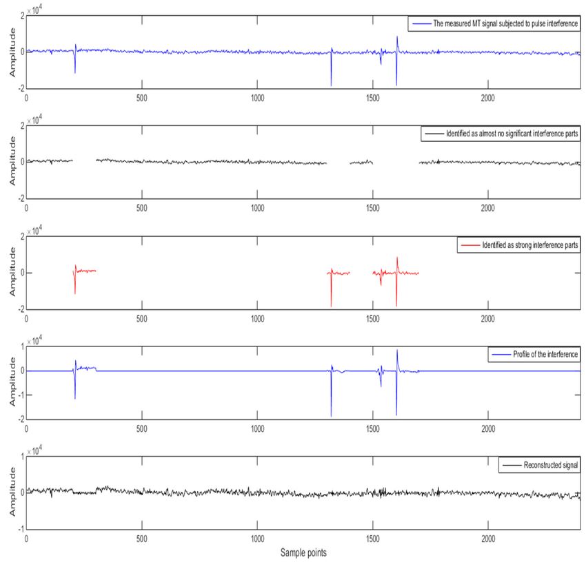
Entropy 2019, 21, 197                                                                                                    6 of 15

3.2. Add Artificial Interference to the Test Site Signal
     To verify the effectiveness of the method, simulated large-scale square wave interference,
triangular wave interference, and pulse interference are added to the test site signal. The test site is
from Qinghai Province, China, located in an area that is far away from any industrial areas, is sparsely
populated, and has almost no external noise pollution. The test site signal is the natural magnetotelluric
signal, which is what we call a signal that is almost unaffected by noise. The result is shown in Figure 2.
         Entropy 2018, 20, x FOR PEER REVIEW                                                                        7 of 17
In Figure 2, “Sample points” refers to the length of data to be processed. Simulated signals have no
temporal resolution
               As can beand   seenonly
                                    fromrepresent    the NCC
                                          Table 1, the    data values
                                                                 length.between
                                                                          Figure the2 shows    that
                                                                                        original testthe
                                                                                                      siteapproximate
                                                                                                           data and the entropy
and multiscale      entropy
         reconstructed           ofare
                            signal  thegreater
                                         samplethanlibrary   signals,
                                                     0.95, and          when they
                                                                the signal-noise       are
                                                                                  ratios areextracted   and
                                                                                             greater than  10. input   to k-means
                                                                                                                Therefore,
         StOMP    has   a good   de-noising  effect and can  effectively retain the  original
clustering, can be used to accurately identify strong interference and useful signals.        useful signal.

                                                              (a)

                                                              (b)

                                                       Figure 2. Cont.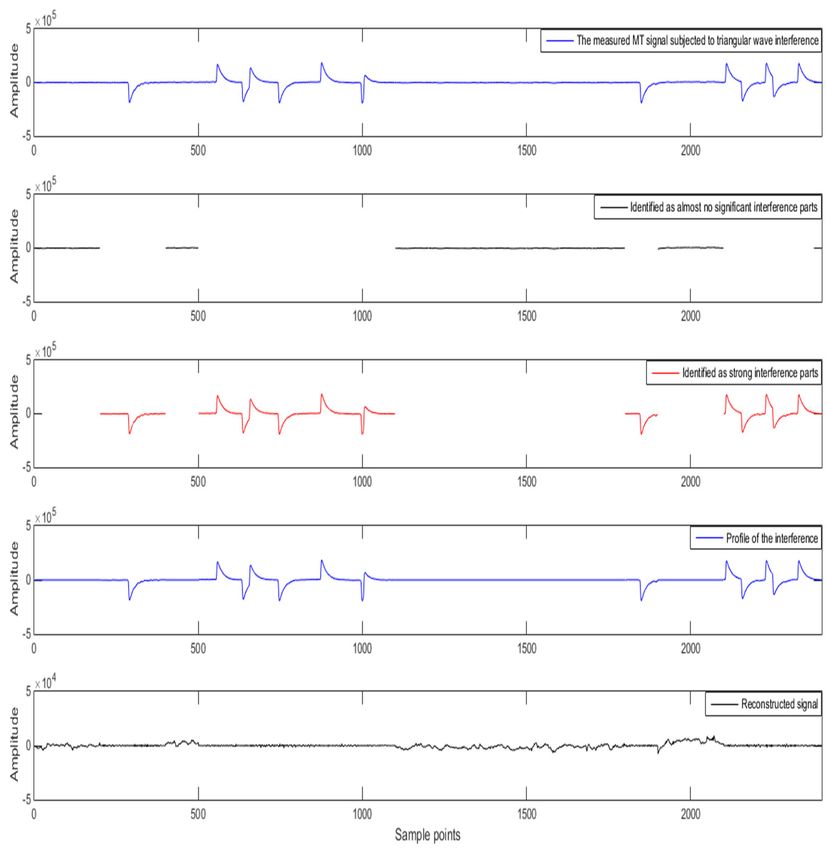
Entropy 2019, 21, 197 7 of 15
Entropy 2018, 20, x FOR PEER REVIEW 8 of 17
(c)
Figure 2.Figure 2. Simulated
Simulated interferencetotoadd
interference add to
tothe
thetest sitesite
test signal with (a)
signal withsquare
(a) wave interference,
square (b)
wave interference,
triangular wave interference, and (c) pulse interference.
(b) triangular wave interference, and (c) pulse interference.
4. Measured Data Analysis
To further illustrate the feasibility of the method proposed herein, normalized cross-correlation
(NCC) [50] and Domain
4.1. Time signal-noise
Analysisratio (SNR) [51] are specifically introduced for the above three types of
interference.Figure
Table3 1shows
compares the two evaluation indicators of the original test site data and the
the signal-noise identification and separation effect of measured MT signals
reconstructed signal.
subjected to square wave interference, triangular wave interference, and pulse interference. These
data are from the Lu-Zong ore-concentration area in Anhui Province, China. For the measured data,
the sampling rate is 24 Hz. 2400Table 1. De-noising
sampling points are performance.
selected for analysis, that is, data is processed
every 100 s. The data are subject to different types and varying degrees of noise interference and they
Type ofofInterference
are used to verify the effectiveness the proposed method. NCC SNR
Square wave interference 0.9775 13.5165
Triangular wave interference 0.9610 11.5246
Pulse interference 0.9852 15.3308
As can be seen from Table 1, the NCC values between the original test site data and the
reconstructed signal are greater than 0.95, and the signal-noise ratios are greater than 10. Therefore,
StOMP has a good de-noising effect and can effectively retain the original useful signal.
4. Measured Data Analysis
4.1. Time Domain Analysis
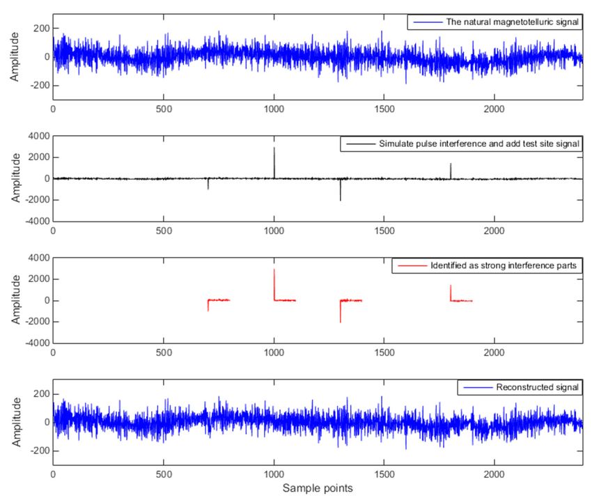
Figure 3 shows the signal-noise identification and separation effect of measured MT signals
subjected to square wave interference, triangular wave interference, and pulse interference. These data
are from the Lu-Zong ore-concentration area in Anhui Province, China. For the measured data,
the sampling rate is 24 Hz. 2400 sampling points are selected for analysis, that is, data is processed
every 100 s. The data are subject to different types and varying degrees of noise interference and they
are used to verify the effectiveness of the proposed method.
Figure 3 shows that the method applied in the measured data processing can still accurately
identify the interfered data segment and effectively suppress the interference. This method avoids the
loss of useful signals and can better preserve the low-frequency slow-change information.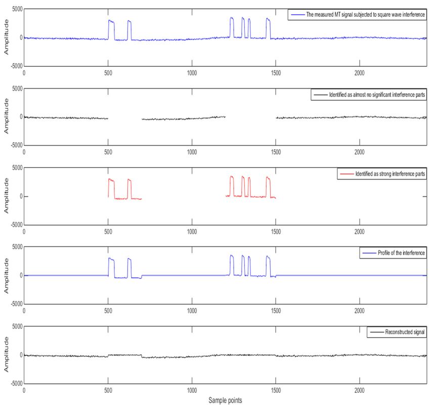
Entropy 2018,21,
Entropy2019,  20,197
                  x FOR PEER REVIEW                     98 of
                                                           of 15
                                                              17

                                            (a)

                                            (b)

                                      Figure 3. Cont.
Entropy 2019, 21, 197 9 of 15
Entropy 2018, 20, x FOR PEER REVIEW 10 of 17
(c)
signal-noise identification
Figure 3. The effect of signal-noise identification and separation for measured magnetotelluric (MT)
interference, (b)
data with (a) square wave interference, (b) triangular
triangular wave
wave interference,
interference, and
and (c)
(c) pulse
pulse interference.
interference.
4.2. Apparent
Figure 3Resistivity-Phase
shows that the Curve Analysis
method applied in the measured data processing can still accurately
identify the interfered data segment and effectively
As the operating frequency decreases, the depth ofsuppress thewill
exploration interference.
gradually This method
increase. avoids
Impedance
the loss of useful signals and can better preserve the low-frequency slow-change information.
values at different frequencies measured on the ground can be used to obtain information about the
resistivity of the subsurface medium as a function of depth. It can be seen that the apparent resistivity
4.2. Apparent
reflects Resistivity-Phase
the comprehensive Curve Analysis
situation of the electrical properties of the rock that can be affected by the
influence of the electromagnetic field
As the operating frequency decreases, in a certain
thefrequency
depth ofrange. When the
exploration willfrequency
gradually is different,
increase.
the range of the influence of the electromagnetic field is different, which reflects
Impedance values at different frequencies measured on the ground can be used to obtain information the resistivity (Ωm)
at different
about depths measuring
the resistivity the signals
of the subsurface medium of different frequencies.
as a function Thus,
of depth. It can beweseen
usethat
the the
trend of the
apparent
apparent resistivity-phase curve as an important indicator to evaluate the degree
resistivity reflects the comprehensive situation of the electrical properties of the rock that can of interference of the
be
measured
affected by sites.
the influence of the electromagnetic field in a certain frequency range. When the
To further
frequency evaluatethe
is different, therange
proposed
of themethod,
influence weofintroduce the data of field
the electromagnetic two measured
is different,sites for
which
reflects the resistivity ( Ωm ) at different depths measuring the signals of different frequencies. Thus,
processing. These two sites are from the Tong-Ling ore-concentration area in Anhui Province, China
and
we useare subject
the trendto different levels of noise
of the apparent interference.curve
resistivity-phase Figures
as 4an
and 5 are the apparent
important indicatorresistivity-phase
to evaluate the
curves of 2535BOAC and 2535BOAF,
degree of interference of the measured sites. respectively.
In
To Figure
further4,evaluate
the blackthe diamonds
proposedare the apparent
method, resistivity-phase
we introduce the data of curve
twoofmeasured
the original
sitesdata.
for
In the 40–0.3 Hz frequency band, the apparent resistivity curve in the R direction
processing. These two sites are from the Tong-Ling ore-concentration area in Anhui Province, China
xy asymptotically
rises to nearly ◦ and the value of the apparent resistivity increases from 100 Ωm to 100,000 Ωm.
and are subject45to ,different levels of noise interference. Figures 4 and 5 are the apparent resistivity-
The
phase above
curvesphenomenon
of 2535BOAC is known as a near-source
and 2535BOAF, effect. If there is no electromagnetic interference
respectively.
around the measured site, the apparent resistivity and phase of the geological structure reflected in
different frequency bands should be relatively stable and should not fluctuate greatly. Due to the
presence of various strong electromagnetic interferences, the noise robustness of the low-frequencyEntropy 2019, 21, 197 10 of 15
band data is obviously worse and thus the result cannot truly reflect the information of 11
Entropy 2018, 20, x FOR PEER REVIEW
a deep
of 17
underground structure.
Figure 4. Comparison of the apparent resistivity-phase curves for site 2535BOAC; the black diamonds,
Figure 4. Comparison of the apparent resistivity-phase curves for site 2535BOAC; the black
blue triangles, and red circles show the apparent resistivity curves obtained from the original
diamonds,
Entropy 2018,the blue PEER
20, overall
x FOR triangles,
REVIEWand red circles show the apparent resistivity curves obtained from the
12 of 17
data, processing of Stagewise orthogonal matching pursuit (StOMP), and the proposed
original data, the overall processing of Stagewise orthogonal matching pursuit (StOMP), and the
method, respectively.
proposed method, respectively.
In Figure 4, the black diamonds are the apparent resistivity-phase curve of the original data. In
the 40—0.3 Hz frequency band, the apparent resistivity curve in the R xy direction asymptotically
rises to nearly 45°, and the value of the apparent resistivity increases from 100 Ωm to 100,000 Ωm
. The above phenomenon is known as a near-source effect. If there is no electromagnetic interference
around the measured site, the apparent resistivity and phase of the geological structure reflected in
different frequency bands should be relatively stable and should not fluctuate greatly. Due to the
presence of various strong electromagnetic interferences, the noise robustness of the low-frequency
band data is obviously worse and thus the result cannot truly reflect the information of a deep
underground structure.
The blue triangles are the apparent resistivity-phase curve after being processed just using the
StOMP algorithm. Although the trend of asymptotic rising of the apparent resistivity curve in the
Rxy direction is alleviated, there is a falling off that occurs in the 3—0.3 Hz frequency band. In the
10—0.3 Hz frequency band, the series of sharp falls in the R yx direction are alleviated, but in the
1—0.3 Hz frequency band, the frequency of the R yx direction is obviously dispersed, showing a
disjointed trend. Compared with the phase curve of the original data, the frequency of the Pyx
direction in the 1—0.3 Hz frequency band is still disorderly and discontinuous.
Figure 5. Comparison of the apparent resistivity-phase curves for site 2535BOAF; the black diamonds,
The red
Figure circles are the
5. Comparison apparent
of the apparentresistivity-phase curvefor
resistivity-phase curves after
site being processed
2535BOAF; bydiamonds,
the black the proposed
blue triangles, and red circles show the apparent resistivity curves obtained from the original data,
method.
blue Comparing
triangles, andthe
redoriginal data the
circles show andapparent
StOMPresistivity
overall processing, the apparent
curves obtained resistivity-phase
from the original data,
the overall processing of StOMP, and the proposed method, respectively.
curvethebecomes smooth and continuous as a whole because the
overall processing of StOMP, and the proposed method, respectively. proposed method retains the low-
frequency slow-change
The blue triangles component without
are the apparent interference while
resistivity-phase curveremoving noise.
after being processed just using the
StOMP In Figure 5, theAlthough
algorithm. black diamonds areof
the trend the apparent resistivity-phase
asymptotic curve resistivity
rising of the apparent of the original
curvedata. In
in the
the
R xy 40—0.3
direction Hzis frequency
alleviated,band,
there the
is a apparent
falling offresistivity
that occurscurve
in the the RHz
in 3–0.3 xy direction
frequency asymptotically
band. In the
rises to nearly 45°. In the 2—0.3 Hz frequency band, the apparent resistivity curve in the R yx
direction is disorderly and shows a downward trend. In the Pyx direction, the phase curve below
10 Hz shows that the phase of some frequency is close to ±180° and the data at these frequencies is
completely distorted.Entropy 2019, 21, 197 11 of 15
10–0.3 Hz frequency band, the series of sharp falls in the Ryx direction are alleviated, but in the 1–0.3 Hz
frequency band, the frequency of the Ryx direction is obviously dispersed, showing a disjointed trend.
Compared with the phase curve of the original data, the frequency of the Pyx direction in the 1–0.3 Hz
frequency band is still disorderly and discontinuous.
The red circles are the apparent resistivity-phase curve after being processed by the proposed
method. Comparing the original data and StOMP overall processing, the apparent resistivity-phase
curve becomes smooth and continuous as a whole because the proposed method retains the
low-frequency slow-change component without interference while removing noise.
In Figure 5, the black diamonds are the apparent resistivity-phase curve of the original data. In the
40–0.3 Hz frequency band, the apparent resistivity curve in the R xy direction asymptotically rises
to nearly 45◦ . In the 2–0.3 Hz frequency band, the apparent resistivity curve in the Ryx direction is
disorderly and shows a downward trend. In the Pyx direction, the phase curve below 10 Hz shows that
the phase of some frequency is close to ±180◦ and the data at these frequencies is completely distorted.
The blue triangles are the apparent resistivity-phase curve after being processed by the StOMP
algorithm. In the 40–0.3 Hz frequency band, compared with the original data, it improved to a certain
degree in the R xy and Ryx directions, and the apparent resistivity value is relatively stable. However,
in the 3–0.3 Hz frequency band, the falling off of the curve in the R xy and Ryx direction is obvious, and
the scattered points in the phase of the Pyx direction increase.
The red circles are the apparent resistivity-phase curve after being processed by the proposed
method. In comparison to the original data and StOMP overall processing, the apparent resistivity
curve of the proposed method is smooth and continuous, and has the least number of scatter points.
4.3. Polarization Direction Analysis
The polarization direction [52] of the electromagnetic field is one of the important indicators used
to evaluate the degree of interference. To further verify the effectiveness of the proposed method,
the polarization direction of the electromagnetic field is calculated and analyzed. Figures 6 and 7
present a comparison of the polarization direction results at 5.2 Hz for site 2535BOAC, and at 2.3 Hz
for site 2535BOAF, respectively.
Entropy 2018, 20, x FOR PEER REVIEW 13 of 17
(a) (b)
Figure
Figure6.6.Comparison
Comparisonof ofthe
thepolarization
polarizationdirection
directionresults
resultsat
at5.2
5.2Hz
Hzfor
forsite
site2535BOAC,
2535BOAC,derived
derivedfrom
from
the
theoriginal
originaldata
data(a)
(a)and
anddata
dataprocessed
processed by
by the
the proposed
proposed method
method (b).
(b).(a) (b)
Entropy 2019, 21, 197
Figure 6. Comparison of the polarization direction results at 5.2 Hz for site 2535BOAC, derived 12 of 15
from
the original data (a) and data processed by the proposed method (b).
(a) (b)
Figure
Figure 7. Comparison
7. Comparison of polarization
of the the polarization direction
direction results
results at Hz
at 2.3 2.3 for
Hz site
for site 2535BOAF,
2535BOAF, derived
derived fromfrom
the original
the original datadata (a) and
(a) and datadata processed
processed by proposed
by the the proposed method
method (b). (b).
According
Accordingto thetodefinition of the polarization
the definition direction ofdirection
of the polarization the electromagnetic field, the polarization
of the electromagnetic field, the
direction is random when there is no strong interference. Otherwise, the polarization
polarization direction is random when there is no strong interference. Otherwise, the polarizationdirection will be
relatively concentrated
direction and regular.
will be relatively As shown
concentrated andinregular.
Figure 6,
Asthe polarization
shown in Figuredirection of the H channel
6, the polarization direction
(magnetic
of the Hfield) is concentrated
channel between
(magnetic field) 70◦ and 90◦ ,between
is concentrated and in Figure
70°and7,90°,
the and
polarization
in Figuredirection of the
7, the polarization
E channel
direction(electric
of thefield) is concentrated
E channel between
(electric field) −60◦ and −90
is concentrated ◦ . The reason is that different types of
between −60°and −90°. The reason is that
strong electromagnetic
different interference
types of strong affect the original
electromagnetic data. Byaffect
interference analyzing the polarization
the original data. Bydirections
analyzing of the
the polarization
data processed by the proposed
directions of the data method, the by
processed polarization directions
the proposed method, of the
the polarization
electric and magnetic
directions of
fields
theare slowlyand
electric scattered
magneticto different
fields aredirections, which isto
slowly scattered close to the directions,
different random characteristics
which is closeof the
to the
natural electromagnetic field. Combined with the apparent resistivity-phase of these two measured
sites at 5.2 Hz and 2.3 Hz in Figures 4 and 5, we can see that the data quality is greatly improved,
preserving more of the useful and reliable underground geoelectric information.
5. Discussion
With the development of society and economy, the demand for energy is increasing. To meet
this demand, we must extend our research efforts to deep underground, using existing technology
to analyze collected data to find more energy and resources. However, various electromagnetic
interferences have also increased, especially in the eastern part of China, where a dense population,
many high-voltage electric wires, communication towers, and highways, etc. severely restrict the
reliability of magnetotelluric data. To obtain more useful and reliable magnetotelluric data, we urgently
need to find a more effective treatment. Most existing methods include the overall processing of
magnetotelluric data, and they lack signal-noise identification. Most importantly, the interference of
many measured sites is not particularly dense. Thus, the overall processing of the magnetotelluric data
is not necessary to avoid the loss of useful information. By observing the time domain waveform of
the measured magnetotelluric data, this can finally be processed in a targeted manner, which preserves
more low-frequency slow-change information for better analysis of the magnetotelluric data.
ApEn and MSE analyses can quantitatively describe the randomness or irregularity of the
magnetotelluric signal and both have good noise robustness. The experimental verification showedEntropy 2019, 21, 197 13 of 15
that the ApEn combined with MSE, used to describe magnetotelluric signals, has obvious advantages.
Figure 1 demonstrates the above points. Two kinds of entropy and k-means clustering were introduced
here to avoid the over-processing of the signal caused by the overall processing and to thereby avoid
losing the important information needed. Figures 2 and 3 illustrate the above. To perform effective
signal-noise separation on magnetotelluric data, we introduced the StOMP algorithm, and Figures 2–5
illustrate the effectiveness of the de-noising. The information of the low-frequency electromagnetic field
can truly reflect the underground distribution information. In addition, we only processed data that
were identified as containing strong interference. The effectiveness of the method is directly reflected
in the effectiveness of the low-frequency data processing and the similarity to the characteristics of the
natural magnetotelluric signals. Figures 4–7 illustrate the problem mentioned above.
The application of the proposed method is based on artificial segmentation of the magnetotelluric
data without adaptive segmentation based on the length of the interfered signal, so it may cause
over-processing of small amounts of data. The StOMP algorithm is required to set the threshold
to update the selected set of atoms for each iteration. However, it is especially difficult to select
this parameter in actual operation. Therefore, in future research, intelligent algorithms, such as
particle swarm optimizations, artificial fish swarm algorithms, and ant colony algorithms, will be
introduced to solve the adaptive segmentation of magnetotelluric data and the threshold selection in
the StOMP algorithm.
6. Conclusions
Natural magnetotelluric signals are extremely weak and irregular relative to a wide variety of
strong interferences. How to identify signal and noise, and extract useful magnetotelluric signals
from strong interference has become an inevitable problem in the field of magnetotelluric sounding.
When faced with massive amounts of measured magnetotelluric data, the distinction of different
signals by ApEn and MSE is still very obvious. Two types of entropy were input to k-means clustering
for signal-noise identification of the magnetotelluric signal, and were used to accurately identify
strong interference and useful signals. Signal-noise separation with the StOMP algorithm was possible
only for data segments identified as containing strong interference. Therefore, the proposed method
effectively ensured identification accuracy and improved de-noising performance. Experiments
showed that the apparent resistivity-phase curve is more continuous and smooth after being processed
by the proposed method, which better preserves the low-frequency slow-change information of the
magnetotelluric signal and greatly improves the data quality. The magnetotelluric data processed
by the proposed method will provide important geoelectric information for subsequent geological
inversion interpretation.
Author Contributions: J.L. and J.T. conceived the idea; J.C. and G.L. designed the experiments; Y.P., X.Z. and C.Z.
helped to analyze the experimental data; J.C. wrote the manuscript; J.L. helped to revise the manuscript.
Acknowledgments: This research was funded by the National Key R&D Program of China (No. 2018YFC0603202),
the National Natural Science Foundation of China (No. 41404111), Natural Science Foundation of Hunan Province
(No. 2018JJ2258) and Hunan Provincial Science and Technology Project Foundation (No. 2018TP1018).
Conflicts of Interest: The authors declare no conflict of interest.
References
1. Cagniard, L. Basic theory of the magnetotelluric method of geophysical prospecting. Geophysics 1953,
18, 605–635. [CrossRef]
2. Tikhonov, A.N. On determining electrical characteristics of the deep layers of the Earth’s crust. Dokl. Akad.
Nauk SSSR 1950, 73, 295–297.
3. He, L.F.; Chen, L.; Dorji; He, Z.X.; Wang, X.B.; Xiao, B.Y.; Xu, L.G.; Zhao, X.F.; Xi, X.L.; Yao, H.C.; et al.
Mapping chromite deposits with audio magnetotellurics in the Luobusa ophiolite of southern Tibet.
Geophysics 2018, 83, B47–B57. [CrossRef]Entropy 2019, 21, 197 14 of 15
4. Ren, Z.Y.; Kalscheuer, T.; Greenhalgh, S.; Maurer, H. A goal-oriented adaptive finite-element approach for
plane wave 3-D electromagnetic modeling. Geophys. J. Int. 2013, 194, 700–718. [CrossRef]
5. Hennessy, L.; Macnae, J. Source-dependent bias of sferics in magnetotelluric responses. Geophysics 2018,
83, E161–E171. [CrossRef]
6. Kappler, K.N. A data variance technique for automated despiking of magnetotelluric data with a remote
reference. Geophys. Prospect. 2012, 60, 179–191. [CrossRef]
7. Li, J.; Zhang, X.; Gong, J.Z.; Tang, J.T.; Ren, Z.Y.; Li, G.; Deng, Y.L.; Cai, J. Signal-noise identification of
magnetotelluric signals using fractal-entropy and clustering algorithm for targeted de-noising. Fractals 2018,
26, 1840011. [CrossRef]
8. Li, J.; Zhang, X.; Tang, J.T.; Cai, J.; Liu, X.Q. Audio magnetotelluric signal-noise identification and separation
based on multifractal spectrum and matching pursuit. Fractals 2019, 27, 1940007. [CrossRef]
9. Huang, Z.X. Extensions to the k-means algorithm for clustering large data sets with categorical values.
Data Min. Knowl. Discov. 1998, 2, 283–304. [CrossRef]
10. Karimov, J.; Ozbayoglu, M. Clustering quality improvement of k-means using a hybrid evolutionary model.
Procedia Comput. Sci. 2015, 61, 38–45. [CrossRef]
11. Rahkar Farshi, T.; Demirci, R.; Feiziderakhshi, M.R. Image clustering with optimization algorithms and color
space. Entropy 2018, 20, 296. [CrossRef]
12. Nielsen, F.; Nock, R.; Amari, S. On clustering histograms with k-Means by Using Mixed α-divergences.
Entropy 2014, 16, 3273–3301. [CrossRef]
13. Wei, M.; Chow, T.W.S.; Chan, R.H.M. Clustering heterogeneous data with k-Means by mutual information-based
unsupervised feature transformation. Entropy 2015, 17, 1535–1548. [CrossRef]
14. Shi, Z.L.; Song, W.Q.; Taheri, S. Improved LMD, permutation entropy and optimized K-Means to fault
diagnosis for roller bearings. Entropy 2016, 18, 70. [CrossRef]
15. Gattone, S.A.; Sanctis, A.D.; Puechmorel, S.; Nicol, F. On the geodesic distance in shapes K-means clustering.
Entropy 2018, 20, 647. [CrossRef]
16. Martin, M.T.; Plastino, A.; Rosso, O.A. Generalized statistical complexity measures: Geometrical and
analytical properties. Phys. A 2006, 369, 439–462. [CrossRef]
17. Pincus, S.M. Approximate entropy as a measure of system complexity. Proc. Natl. Acad. Sci. USA 1991,
88, 2297–2301. [CrossRef]
18. Richman, J.S.; Moorman, J.R. Physiological time-series analysis using approximate entropy and sample
entropy. Am. J. Physiol. Heart Circ. Physiol. 2000, 278, H2039–H2049. [CrossRef]
19. Costa, M.; Goldberger, A.L.; Peng, C.K. Multiscale entropy analysis of complex physiologic time series.
Phys. Rev. Lett. 2002, 89, 068102. [CrossRef]
20. Costa, M.; Goldberger, A.L.; Peng, C.K. Multiscale entropy analysis of biological signals. Phys. Rev. E 2005,
71, 021906. [CrossRef]
21. Kaplanis, P.A.; Pattichis, C.S.; Zazula, D. Multiscale entropy-based approach to automated surface EMG
classification of neuromuscular disorders. Med. Biol. Eng. Comput. 2010, 48, 773–781.
22. Wu, S.D.; Wu, C.W.; Wu, T.Y.; Wang, C.C. Multi-scale analysis based ball bearing defect diagnostics using
Mahalanobis distance and support vector machine. Entropy 2013, 15, 416–433. [CrossRef]
23. Humeau-Heurtier, A. The multiscale entropy algorithm and its variants: A review. Entropy 2015, 17, 3110–3123.
[CrossRef]
24. Mayer, C.; Bachler, M.; Hörtenhuber, M.; Stocker, C.; Holzinger, A.; Wassertheurer, S. Selection of
entropy-measure parameters for knowledge discovery in heart rate variability data. BMC Bioinform. 2014,
15, S2. [CrossRef]
25. Manis, G.; Aktaruzzaman, M.; Sassi, R. Bubble entropy: An entropy almost free of parameters. IEEE Trans.
Biomed. Eng. 2017, 64, 2711–2718.
26. Donoho, D.L. Compressed Sensing. IEEE Trans. Inf. Theory 2006, 52, 1289–1306. [CrossRef]
27. Donoho, D.L.; Maleki, A.; Motanari, A. Message passing algorithms for compressed sensing. Proc. Natl.
Acad. Sci. USA 2009, 106, 18914–18919. [CrossRef]
28. Donoho, D.L.; Tanner, J. Precise undersampling theorems. Proc. IEEE 2010, 98, 913–924. [CrossRef]
29. Donoho, D.L.; Johnstone, I.; Montanari, A. Accurate prediction of phase transitions in compressed sensing
via a connection to minimax denoising. IEEE Trans. Inf. Theory 2013, 59, 3396–3433. [CrossRef]Entropy 2019, 21, 197 15 of 15
30. Mallat, S.G.; Zhang, Z. Matching pursuits with time-frequency dictionaries. IEEE Trans. Signal Process. 1993,
41, 3397–3415. [CrossRef]
31. Li, J.; Yan, H.; Tang, J.T.; Zhang, X.; Li, G.; Zhu, H.J. Magnetotelluric noise suppression based on matching
pursuit and genetic algorithm. Chin. J. Geophys. 2018, 61, 3086–3101.
32. Needell, D.; Vershynin, R. Uniform uncertainty principle and signal recovery via regularized orthogonal
matching pursuit. Found. Comput. Math. 2009, 9, 317–334. [CrossRef]
33. Needell, D.; Vershynin, R. Signal recovery from incomplete and inaccurate measurements via regularized
orthogonal matching pursuit. IEEE J. Sel. Top. Signal Process. 2010, 4, 310–316. [CrossRef]
34. Burioka, N.; Cornelisson, G.; Halberg, F.; Kaplan, D.T.; Suyama, H.; Sako, T.; Shimizu, E.I. Approximate
entropy of human respiratory movement during eye-closed waking and different sleep stages. Chest 2003,
123, 80–86. [CrossRef]
35. Pincus, S. Approximate entropy as an irregularity measure for financial data. Econom. Rev. 2008, 27, 329–362.
[CrossRef]
36. Zhang, Z.; Chen, Z.; Zhou, Y.; Du, S.; Zhang, Y.; Mei, T.; Tian, X. Construction of rules for seizure prediction
based on approximate entropy. Clin. Neurophysiol. 2014, 125, 1959–1966. [CrossRef]
37. Mei, T.; Qiao, J.D.; Zhou, Y.; Gu, H.Y.; Chen, Z.Y.; Tian, X.H.; Gu, K.Y. Analysis of neural oscillations on
Drosophila’s subesophageal ganglion based on approximate entropy. Entropy 2015, 17, 6854–6871. [CrossRef]
38. Manis, G.; Aktaruzzaman, M.; Sassi, R. Low computational cost for sample entropy. Entropy 2018, 20, 61.
[CrossRef]
39. Karevan, Z.; Suykens, J.A.K. Transductive Feature selection using clustering-based sample entropy for
temperature prediction in weather forecasting. Entropy 2018, 20, 264. [CrossRef]
40. Bakhchina, A.V.; Arutyunova, K.R.; Sozinov, A.A.; Demidovsky, A.V.; Alexandrov, Y.I. Sample Entropy of
the heart rate reflects properties of the system organization of behaviour. Entropy 2018, 20, 449. [CrossRef]
41. Ahmadi, S.; Sepehri, N.; Wu, C.; Szturm, T. Sample entropy of human gait center of pressure displacement:
A Systematic Methodological Analysis. Entropy 2018, 20, 579. [CrossRef]
42. McCamley, J.D.; Denton, W.; Arnold, A.; Raffalt, P.C.; Yentes, J.M. On the calculation of sample entropy using
continuous and discrete human gaitdata. Entropy 2018, 20, 764. [CrossRef]
43. Trybek, P.; Nowakowsuki, M.; Salowka, J.; Spiechowicz, J.; Machura, L. Sample entropy of sEMG signals at
different stages of rectal cancer treatment. Entropy 2018, 20, 863. [CrossRef]
44. Chou, C.M. Wavelet-based multi-scale entropy analysis of complex rainfall time series. Entropy 2011,
13, 241–253. [CrossRef]
45. Hong, T.; Zhang, X.; Ma, H.J.; Chen, Y.; Chen, X. Fatiguing effects on the multi-scale entropy of surface
electromyography in children with cerebral palsy. Entropy 2016, 18, 177. [CrossRef]
46. Wu, T.Y.; Yu, C.L.; Liu, D.C. On Multi-scale entropy analysis of order-tracking measurement for bearing fault
diagnosis under variable speed. Entropy 2016, 18, 292. [CrossRef]
47. Pham, T.D. Time-shift multiscale entropy analysis of physiological signals. Entropy 2017, 19, 257. [CrossRef]
48. Donoho, D.L.; Tsaig, Y.; Drori, I.; Starck, J.L. Sparse solution of underdetermined systems of linear equations
by stagewise orthogonal matching pursuit. IEEE Trans. Inform. Theory 2012, 58, 1094–1121. [CrossRef]
49. Li, J.; Tang, J.T.; Xu, Z.M.; Yan, H. Magnetotelluric noise suppression base on signal-to-noise identification in
ore concentration area. Chin. J. Geophys. 2017, 60, 722–737.
50. Amaralsilva, H.; Wichertana, L.; Murta, L.O.; Romualdosuzuki, L.; Itikawa, W.; Bussato, G.F.;
Azevedomarques, P. The superiority of tsallis entropy over traditional cost functions for brain MRI and
SPECT registration. Entropy 2014, 16, 1632–1651. [CrossRef]
51. Li, G.; Xiao, X.; Tang, J.T.; Li, J.; Zhu, H.J.; Zhou, C.; Yan, F.B. Near-source noise suppression of AMT by
compressive sensing and mathematical morphology filtering. Appl. Geophys. 2017, 14, 581–589. [CrossRef]
52. Weckmann, U.; Magunia, A.; Ritter, O. Effective noise separation for magnetotelluric single site data
processing using a frequency domain selection scheme. Geophys. J. Int. 2005, 161, 635–652. [CrossRef]
© 2019 by the authors. Licensee MDPI, Basel, Switzerland. This article is an open access
article distributed under the terms and conditions of the Creative Commons Attribution
(CC BY) license (http://creativecommons.org/licenses/by/4.0/).You can also read


