Monitoring-Well Installation, Slug Testing, and Groundwater Quality for Selected Sites in South Park, Park County, Colorado, 2013
←
→
Page content transcription
If your browser does not render page correctly, please read the page content below
Prepared in cooperation with Park County, Colorado

Monitoring-Well Installation, Slug Testing, and Groundwater
Quality for Selected Sites in South Park, Park County,
Colorado, 2013
By L.R. Arnold

Open-File Report 2014–1231

U.S. Department of the Interior
U.S. Geological Survey
U.S. Department of the Interior
SALLY JEWELL, Secretary
U.S. Geological Survey
Suzette M. Kimball, Acting Director
U.S. Geological Survey, Reston, Virginia: 2015
For more information on the USGS—the Federal source for science about the Earth,
its natural and living resources, natural hazards, and the environment—visit
http://www.usgs.gov or call 1–888–ASK–USGS (1–888–275–8747)
For an overview of USGS information products, including maps, imagery, and publications,
visit http://www.usgs.gov/pubprod
To order this and other USGS information products, visit http://store.usgs.gov
Any use of trade, firm, or product names is for descriptive purposes only and does not imply
endorsement by the U.S. Government.
Although this information product, for the most part, is in the public domain, it also may
contain copyrighted materials as noted in the text. Permission to reproduce copyrighted items
must be secured from the copyright owner.
Suggested citation:
Arnold, L.R., 2015, Monitoring-well installation, slug testing, and groundwater quality for selected sites in South Park,
Park County, Colorado, 2013: U.S. Geological Survey Open-File Report 2014–1231, 32 p.,
http://dx.doi.org/10.3133/ofr20141231.
ISSN 2331-1258 (online)
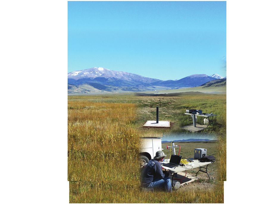
Cover photographs. Background: View looking north from near Garo, Colorado. Left-center: Typical monitoring-well
installation. Right-center: Typical setup used to monitor field properties prior to water-quality sampling, South Park,
Colorado. Bottom right: U.S. Geological Survey hydrologist monitoring water-level response to an air-pressurized slug
test, South Park, Colorado.
ii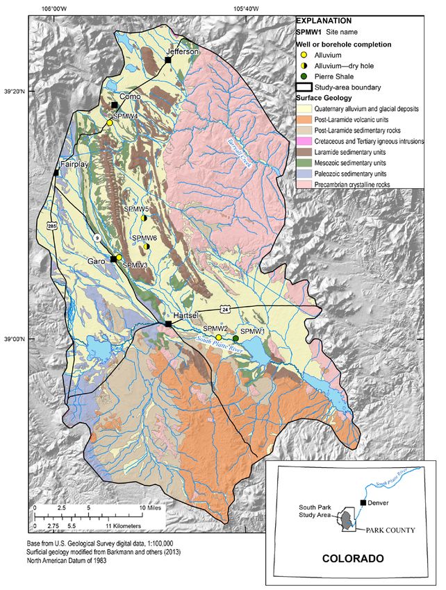
Contents
Abstract ......................................................................................................................................................................... 1
Introduction .................................................................................................................................................................... 1
Monitoring-Well Installation............................................................................................................................................ 4
Slug Testing................................................................................................................................................................... 7
   Field Methods ............................................................................................................................................................ 7
     Air-Pressurized Slug Tests ..................................................................................................................................... 7
     Mechanical Slug Tests ..........................................................................................................................................10
   Analytical Methods ....................................................................................................................................................10
     Slug-Test Solutions ...............................................................................................................................................10
        KGS Model ........................................................................................................................................................10
        Peres-Onur-Reynolds Approximate Deconvolution Method...............................................................................10
     Data Processing and Analysis ...............................................................................................................................11
   Hydraulic-Conductivity Estimates ..............................................................................................................................22
Groundwater Quality .....................................................................................................................................................22
   Sample Collection and Processing ...........................................................................................................................22
   Quality Control ..........................................................................................................................................................23
   Analytical Results......................................................................................................................................................23
     Field Measurements, Major Ions, Nutrients, Trace Elements, and Organic Carbon ..............................................23
     Volatile Organic Compounds, Ethane, Methane, and Radon ................................................................................26
Summary ......................................................................................................................................................................29
Acknowledgments ........................................................................................................................................................30
References Cited ..........................................................................................................................................................30
Appendix 1.Lithologic Logs ......................................................................................................................................... link
Appendix 2.Well-Construction Diagrams .................................................................................................................... link
Appendix 3.Well-Development Records ..................................................................................................................... link
Appendix 4.Water-Quality Control Data ...................................................................................................................... link

Figures
Figure 1. Locations of monitoring wells and boreholes drilled in South Park, Colorado, 2013. ................................. 3
Figure 2. Equipment used for conducting air-pressurized slug tests on monitoring wells installed in
South Park, Colorado, 2013 .......................................................................................................................................... 9
Figure 3. Normalized displacement relative to time for slug tests conducted at each well (SPMW1–4)
installed in South Park, Colorado, 2013....................................................................................................................... 16
Figure 4. Equivalent drawdown relative to time and straight-line match using the approximate deconvolution
method of Peres and others (1989) for four slug tests performed at well SPMW1, September 24, 2013 .................... 18
Figure 5. Normalized displacement relative to time and type-curve match using the KGS model (Hyder and
others, 1994) for four slug tests performed at well SPMW2, September 24, 2013 ...................................................... 19
Figure 6. Normalized displacement relative to time and type-curve match using the KGS model (Hyder and
others, 1994) for four slug tests performed at well SPMW3, September 25, 2013 ...................................................... 20
Figure 7. Normalized displacement relative to time and type-curve match using the KGS model (Hyder and
others, 1994) for four slug tests performed at well SPMW4, September 23, 2013 ...................................................... 21
Figure 8. Trilinear diagram showing major-ion composition of groundwater samples collected from monitoring
wells (SPMW1–4) installed in South Park, Colorado, 2013 ......................................................................................... 25

                                                                                        iii
Tables
Table 1. Summary of location, construction, and hydrogeologic information for groundwater monitoring wells
installed in South Park, 2013 ......................................................................................................................................... 6
Table 2. Summary of aquifer material, displacement method, and dimensions used for slug-test analyses
conducted on monitoring wells installed in South Park, 2013 ...................................................................................... 12
Table 3. Analysis method, displacement method, expected and actual initial displacement, and estimated
hydraulic conductivity of aquifer materials in screen interval of monitoring wells installed in South Park, 2013 .......... 14
Table 4. Field measurements, major-ion, nutrient, trace-element, and organic-carbon data for monitoring
wells installed in South Park, 2013 .............................................................................................................................. 24
Table 5. Volatile-organic-compound, ethane, methane, and radon data for monitoring wells installed in
South Park, 2013 ......................................................................................................................................................... 27
Conversion Factors
Inch/Pound to SI
Multiply By To obtain
Length
inch (in.) 25.4 millimeter (mm)
foot (ft) 0.3048 meter (m)
Flow rate
gallon per minute (gal/min) 0.06309 liter per second (L/s)
Pressure
pound per square inch (lb/in2) 6.895 kilopascal (kPa)
2
pound per square inch (lb/in ) 2.307 feet of water (ft)
Hydraulic conductivity
foot per day (ft/d) 0.3048 meter per day (m/d)
SI to Inch/Pound
Multiply By To obtain
Length
millimeter (mm) 0.03937 inch (in.)
Temperature in degrees Celsius (°C) may be converted to degrees Fahrenheit (°F) as follows:
°F=(1.8×°C)+32
Vertical coordinate information is referenced to the North American Vertical Datum of 1988 (NAVD 88).
Horizontal coordinate information is referenced to the North American Datum of 1983 (NAD 83).
Altitude, as used in this report, refers to distance above the vertical datum.
Specific conductance is given in microsiemens per centimeter at 25 degrees Celsius (µS/cm at 25 °C).
ivAbbreviations
CUSP Coalition for the Upper South Platte
DOC dissolved organic carbon
ID inside diameter
KGS Kansas Geological Survey
MCL maximum contaminant levels
N normal
NWIS National Water Information System
NWQL National Water Quality Laboratory
PVC polyvinyl chloride
SMCL secondary maximum contaminant levels
USGS U.S. Geological Survey
VOC volatile organic compounds
vMonitoring-Well Installation, Slug Testing, and
Groundwater Quality for Selected Sites in South Park,
Park County, Colorado, 2013
By L.R. Arnold
Abstract
During May–June, 2013, the U.S. Geological Survey, in cooperation with Park County,
Colorado, drilled and installed four groundwater monitoring wells in areas identified as needing new
wells to provide adequate spatial coverage for monitoring water quality in the South Park basin.
Lithologic logs and well-construction reports were prepared for each well, and wells were developed
after drilling to remove mud and foreign material to provide for good hydraulic connection between the
well and aquifer. Slug tests were performed to estimate hydraulic-conductivity values for aquifer
materials in the screened interval of each well, and groundwater samples were collected from each well
for analysis of major inorganic constituents, trace metals, nutrients, dissolved organic carbon, volatile
organic compounds, ethane, methane, and radon. Documentation of lithologic logs, well construction,
well development, slug testing, and groundwater sampling are presented in this report.
Introduction
South Park is a high-altitude intermontane basin in Park County, Colorado (fig. 1), that
comprises part of the upper South Platte River watershed and contains important groundwater resources.
The geology of the South Park basin is complex, and groundwater within the basin occurs in alluvial,
sedimentary-bedrock, and crystalline-rock aquifers (Lewis, 2000). Alluvial aquifers in South Park occur
within discontinuous Quaternary deposits consisting of glacial drift and outwash along with post-glacial
sediments associated with modern stream systems (fig. 1; Barkmann and others, 2013). Sedimentary-
bedrock aquifers underlie alluvium in most areas of the basin and generally consist of eastward-dipping
Paleozoic, Mesozoic, and Cenozoic (Laramide and post-Laramide) rocks composed primarily of
sandstone, siltstone, conglomerate, and limestone separated by layers of shale or volcanic rocks.
Crystalline-rock aquifers occur primarily in uplifted Precambrian igneous and metamorphic rocks on the
east side of the basin, but they also are present within post-Laramide volcanic rocks in the southern part
of the basin and in small areas of Cretaceous and Tertiary igneous intrusions. The structure of the basin
has been affected by thrust faulting, folding, and possible strike-slip faulting with widespread zones of
deformation (Barkmann and others, 2013).
In early 2013, to address concerns about managing groundwater resources and protecting water
quality from potential oil and gas development in the basin, the U.S. Geological Survey (USGS), in
cooperation with Park County, participated with the Colorado Geological Survey and the Coalition for
the Upper South Platte (CUSP) in a scoping study (Barkmann and others, 2013) to assess current
hydrogeologic understanding of the South Park basin, develop a framework for more comprehensive
1future hydrogeologic studies, and design a well network for long-term monitoring of groundwater
quality in the South Park basin. The network utilized existing wells wherever possible but identified
locations where new wells were needed to provide adequate spatial coverage for monitoring water
quality in the South Park basin. Details concerning the regional hydrogeology of South Park and
locations of existing wells utilized in the full network are presented by Barkmann and others (2013).
2Figure 1. Locations of monitoring wells and boreholes drilled in South Park, Colorado, 2013.
3In May 2013, the USGS entered into a second cooperative agreement with Park County to install
six groundwater monitoring wells in areas identified by the scoping study as needing new wells to
provide adequate spatial coverage for monitoring water quality in the South Park basin. Five wells were
planned for completion in priority areas of unconsolidated alluvial deposits, and one well was planned
for completion in bedrock materials. Specific objectives of the project were as follows:
1. Install six monitoring wells at locations identified in the scoping study as important for
monitoring water quality near areas of potential oil and gas development and where existing
water wells are not present,
2. Conduct slug tests on each completed well to estimate aquifer hydraulic conductivity at each
site, and
3. Collect groundwater samples from each completed well to provide baseline water-quality data
representative of conditions prior to extensive oil and gas development in the basin.
Well drilling during May–June 2013, however, encountered unsaturated (dry) alluvium at two of
the planned alluvial-monitoring-well locations, so that only four wells (three alluvial wells and one
bedrock well) were installed. The bedrock well was installed in a sandstone layer of the Pierre Shale.
The purpose of this report is to document data related to the installation, slug testing, and
groundwater sampling of monitoring wells added to the well network designed by the scoping study to
monitor water quality in the South Park basin.
Monitoring-Well Installation
Monitoring wells initially were sited on the basis of locations identified in the scoping study by
Barkmann and others (2013) as important for establishing new wells to monitor water quality in the
South Park basin. Landowners were contacted by CUSP to request permission to drill and install wells
as close as possible to the sites selected by the scoping study. Final well locations (fig. 1) ultimately
depended on site conditions and landowner permission for access. Because landowner permission could
not be obtained for the original location planned for the bedrock well about 2 miles north of Hartsel,
another important monitoring location was selected about 6 miles east of Hartsel downgradient from
areas of potential oil and gas development shown by Barkmann and others (2013).
Drilling and monitoring-well installation were performed May 29 through June 3, 2013, by the
USGS. An onsite USGS geologist was responsible for documenting daily drilling operations, logging
and packaging geologic materials from drill holes, overseeing well installation, and preparing well-
construction reports. CUSP was responsible for applying for permits required by the State of Colorado
for well drilling.
Boreholes for the monitoring wells were drilled using a truck-mounted CME85 drilling rig.
Boreholes for alluvial wells SPMW2, SPMW3, and SPMW4 were drilled with 4.25-inch inside
diameter (ID) hollow-stem augers to the total depth of the borehole. Similarly, boreholes for planned
alluvial wells SPMW5 and SPMW6 were drilled with 4.25-inch ID hollow-stem augers; however,
monitoring wells were not completed in these boreholes because the alluvium and underlying bedrock
were dry to the depths drilled. The borehole for the bedrock well SPMW1 was drilled to a depth of 30
feet with 6.25-inch ID hollow-stem augers, at which point the drilling method was changed to air rotary
with 6-inch outside diameter solid-stem augers to continue advancement of the borehole through
competent bedrock to the total borehole depth. A single 5-foot core sample was collected near the
bottom of the borehole for well SPMW1 in the interval from 198.5 to 201.7 feet (3.2 feet of recovery) in
a silty sandstone layer for the purpose of evaluating the suitability of completing the well at this depth.
Although planned for completion at a depth of about 200 feet, inspection of the core and cuttings
4collected for well SPMW1 indicated little or no saturation below a silty sandstone layer from about 31
to 44 feet below land surface that resulted in a decision to complete the well at a shallower depth than
planned. Alluvium overlying bedrock at site SPMW1 was dry except for about 0.5 foot of saturation
perched on top of the weathered bedrock surface. With exception of the single core sample from well
SPMW1, lithologic descriptions (appendix 1) for each borehole were made on the basis of visual
inspection of auger cuttings. Grain size was described on the basis of the Wentworth classification
system (Wentworth, 1922). Unconsolidated materials (top soil and alluvium) at the sites were found to
range from 5 to 19 feet thick. However, the full thickness of alluvium at well SPMW3 is not known
because drilling did not reach bedrock at the site. Drilling augers, rods, and bits were cleaned with a
pressure washer after completing each borehole to minimize the potential for transporting chemical
constituents offsite and introducing them to subsequent boreholes.
Well-construction diagrams for the monitoring wells are presented in appendix 2, and well-
completion details are summarized in table 1. Total borehole depths range from 8.9 to 201.7 feet below
land surface with well depths ranging from 8.9 to 48.6 feet below land surface. Groundwater levels
measured in the wells immediately after installation ranged from 2.8–7.6 feet below land surface. All
wells are constructed of 2-inch nominal diameter, Schedule 40, threaded and flush-jointed polyvinyl
chloride (PVC) well casing with 5- or 10-foot-long screens having 0.01-inch slots. A 0.5-foot-long
threaded well point was used to complete the bottom of each well. The annular space adjacent to the
screened interval was backfilled with 10–20 mesh silica sand, and the annular space above the sand
pack was sealed with bentonite and (or) cement-bentonite grout to near land surface. The open borehole
below 48.6 feet at well SPMW1 was sealed with bentonite prior to setting the well casing. All wells
were completed at the land surface with a 4-foot square concrete pad surrounding the well and a
protective steel surface casing with locking lid. Well construction was in accordance with USGS
specifications for water-quality wells (Lapham and others, 1997) and water-well construction rules for
the State of Colorado (http://water.state.co.us/DWRIPub/Documents/constructionrules05.pdf, accessed
May 20, 2013).
5Table 1. Summary of location, construction, and hydrogeologic information for groundwater monitoring wells installed in South Park, 2013.
[USGS, U.S. Geological Survey; DDMMSS.S, degrees, minutes, decimal seconds; land-surface altitude in feet; all depths in feet below land surface]
Local Land- Depth Depth to Depth to Depth to Depth to
USGS Latitude1 Longitude1 Date Hole Well Hydrogeologic
well surface to top of bottom of top of bottom of
site number (DDMMSS.S) (DDMMSS.S) drilled depth depth completion
name altitude2 water3 screen screen sand pack sand pack
SPMW1 390010105404901 390010.3 1054048.6 8,712 06/01/2013 201.7 7.6 48.6 33.3 43.1 30.3 48.6 Pierre Shale
SPMW2 390014105423401 390014.4 1054234.0 8,740 06/02/2013 8.9 3.1 8.9 3.6 8.4 3.0 8.9 Alluvium
SPMW3 390639105525701 390638.6 1055257.2 9,167 06/03/2013 19.0 2.9 19.0 8.7 18.5 6.5 19.0 Alluvium
SPMW4 391731105540501 391730.8 1055404.8 9,636 06/03/2013 17.0 2.8 16.0 10.7 15.5 10.6 17.0 Alluvium
1
Latitude and longitude determined by global positioning system. North American Datum of 1983.
2
Land-surface altitude estimated from U.S. Geological Survey (2011). North American Vertical Datum of 1988.
3
Measured at time of drilling.
6Wells were developed after drilling to remove mud and any foreign material from the well and to
help improve the hydraulic connection between the well and aquifer. Preliminary well development was
completed after drilling June 1–3, 2013, by using a mechanical bailer attached to the drill rig. Further
well development was accomplished June 4–5 and June 17, 2013, by using a combination of pumping
and mechanical surging with a Waterra PowerPump-2 (wells SPMW1 and SPMW2) or Hydrolift-2
(wells SPMW3 and SPMW4) inertial pump system for a maximum of about 5 hours or until the
produced water was clear and specific conductance was stable.
Slug Testing
A slug test is a method of estimating hydraulic properties of aquifer materials in the immediate
vicinity of a well by measuring the water-level response in a well after a near-instantaneous change in
hydraulic head. Slug tests can be initiated by adding or removing water or a solid object (mechanical
slug) to the water column or by changing air pressure in the well casing above the static water level
(Cunningham and Schalk, 2011). Because slug tests are sensitive to near-well conditions, they can be
strongly affected by well- skin effects (borehole alteration of aquifer properties caused by well drilling,
installation, and development; Butler, 1998).
Field Methods
Slug tests were performed September 23–25, 2013, after water levels had stabilized from drilling
and well development. Two slug-testing methods were used to estimate hydraulic-conductivity values of
aquifer materials in the screen intervals of completed wells. Air-pressurized slug tests were performed
on wells SPMW1, SPMW3, and SPMW4. Because a near-instantaneous pressurization of the well was
not achieved during air-pressurized slug tests, falling-head data were not collected for these tests and
only the rising-head portion of the tests were used for analysis. Because the static water level in well
SPMW2 was only slightly above the screen interval, mechanical slugs were used to perform falling-
head slug tests on well SPMW2 to avoid displacing the water level to below the top of the screen
interval during testing. Mechanical slugs also were used at well SPMW3 to perform both rising- and
falling-head tests because results of air-pressurized slug tests appeared problematic.
Prior to initiating slug tests, the static water level was measured with an electric water-level tape,
and a submersible pressure transducer (Global Water Instrumentation, Inc., model WL16, range 0–15
feet, 0.1 percent accuracy at constant temperature) was placed in the well at a depth below any
anticipated mechanical slug insertion and the lowest expected water level for each test. After placement
in the well, the temperature of the pressure transducer was allowed several minutes to equilibrate to the
prevailing groundwater temperature. Pressure transducers were checked for proper calibration by
comparing readings to manual measurements in a column of water prior to deploying them to the field.
During slug testing, hydraulic head was recorded every 0.1 second by the pressure transducer, and water
levels were allowed greater than or equal to 98 percent recovery before terminating each test. Each well
was tested at least four times using two different initial displacements to verify results and assist in
assessing slug-test response and analysis methods as described by Butler (1998).
Air-Pressurized Slug Tests
Air-pressurized slug tests were initiated by pressurizing the airspace in the well casing to depress
the water column to a new equilibrium level. After hydraulic-head readings stabilized, pressure was
released instantaneously from the well, and transducer readings were monitored until the water level
returned to near its static position. Greene and Shapiro (1995) provide a detailed description of methods
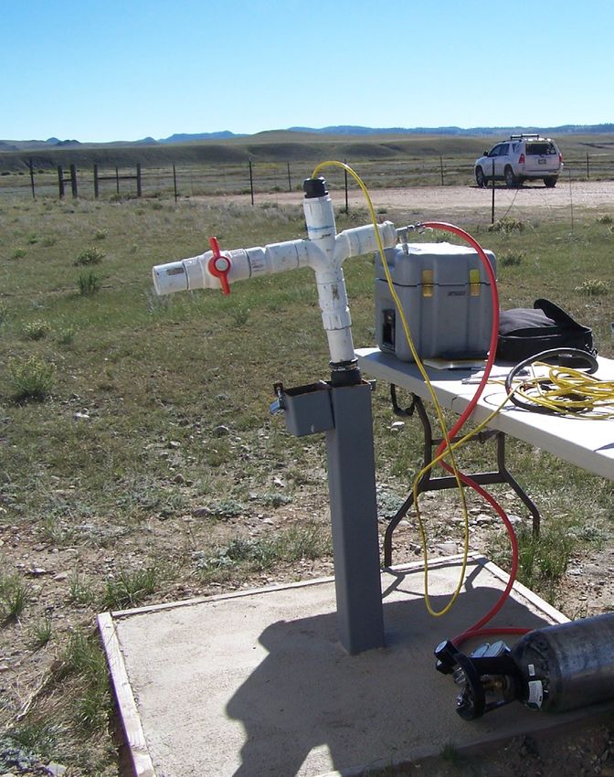
7used for performing air-pressurized slug tests. Pressurization of the well was achieved by using
compressed nitrogen and a well-head apparatus (fig. 2) designed for conducting air-pressurized slug
tests. A pressure regulator and gage (Swagelok unfilled industrial type, range 0–30 psi, accuracy 1.5
percent of full range) connected between the compressed nitrogen tank and well-head apparatus were
used to regulate and monitor the applied air pressure.
8Transducer cable
Well-head apparatus
Pressure regulator and gage
Nitrogen tank
Figure 2. Equipment used for conducting air-pressurized slug tests on monitoring wells installed in South Park,
Colorado, 2013.
9Mechanical Slug Tests
Mechanical slug tests were performed using standardized techniques for conducting slug tests
with a mechanical slug and submersible pressure transducer (Cunningham and Schalk, 2011). For each
falling-head test, the slug was lowered rapidly below the water surface in the well causing a near-
instantaneous rise in the water level, and transducer (hydraulic head) readings were monitored until the
water level returned to near its static position. For each rising-head test, the slug was quickly removed
from the well, causing a near-instantaneous drop in the water level, and transducer (hydraulic head)
readings were monitored until the water level returned to near its static position. Mechanical slugs used
for the tests are made of solid PVC with tapered ends exceeding an 80-degree angle (Midwest
Geosciences Group, Solid H(o) Slug).
Analytical Methods
Slug-Test Solutions
Response data were analyzed using one of two slug-test solutions selected on the basis of well
and aquifer conditions at each site and as implemented by the computer program AQTESOLV
(HydroSOLV, Inc., 2013)—the KGS (Kansas Geological Survey) model or the Peres-Onur-Reynolds
approximate deconvolution method.
KGS Model
The KGS model (Hyder and others, 1994) was used to analyze data collected at wells SPMW2,
SPMW3, and SPMW4. It is a semianalytical solution developed by the Kansas Geological Survey for
analyzing slug-test data from wells screened in confined or unconfined aquifers. The model incorporates
the effects of partial penetration, anisotropy, finite-radius well skins, and upper and lower aquifer
boundaries, and aquifer materials are assumed to be homogeneous. Application of the KGS model
involves plotting normalized water-level displacement (water-level displacement divided by initial
displacement) relative to the logarithm of time and comparing the plot to a set of type curves for
estimation of values for hydraulic conductivity and specific storage.
Peres-Onur-Reynolds Approximate Deconvolution Method
The Peres-Onur-Reynolds approximate deconvolution method (Peres and others, 1989) was used
to analyze data collected at well SPMW1. The method is based on converting slug-test response data
into equivalent hydraulic-head (equivalent drawdown) data that would result from a constant-rate
pumping test at a well having well-bore storage and skin effects. The equivalent drawdown data can
then be analyzed using the Cooper-Jacob semilog straight-line method (Cooper and Jacob, 1946) for
constant-rate pumping tests. The model assumptions are that the aquifer is confined and that aquifer
materials are homogeneous, isotropic, and of uniform thickness. Conversion of slug-test data to
equivalent drawdown by using the method is valid for all well-aquifer geometries (Peres and others,
1989), including partially-penetrating wells. The technique works best when initial displacement is
large, high-accuracy pressure transducers are used, background noise is small, and the test is run to
complete recovery (Butler, 1998). The method can often produce a reasonable estimate of hydraulic
conductivity near fully penetrating wells with skins having a lower hydraulic conductivity than the
surrounding aquifer.
10Data Processing and Analysis
To facilitate analysis, raw data were processed so that data displayed a logarithmic decrease in
sample frequency from one reading every 0.1 second at the start of the test to one reading every 10
seconds for later parts of the test. Early-time (prior to about 2 seconds) noise in data collected during
slug tests performed using mechanical slugs likely is the result of dynamic pressure effects from
introducing or removing the slugs (described by Butler, 1998) and was ignored in the analysis.
Aquifer conditions were considered to be unconfined with the exception of well SPMW1, which
was completed in a sandstone layer of the Pierre Shale below 23 feet of clay within the weathered Pierre
Shale (appendix 1). Because the bottom of the screen interval for wells SPMW2 and SPMW4 are
located below the aquifer base, the screen interval for these wells was taken as the distance between the
top of the screen and the base of the aquifer, rather than the actual screen length. Although the actual
depth is unknown, the aquifer base at well SPMW3 was assumed to be 1 foot below the bottom of well.
For all tests, the borehole radius was used to represent the radius of the screen interval, and the radius of
the transducer cable (0.013 foot) was considered in the computation of an effective casing radius. A
summary of dimensions used for the calculation of each slug test is provided in table 2.
11Table 2. Summary of aquifer material, displacement method, and dimensions used for slug-test analyses conducted on monitoring wells installed in
South Park, 2013.
[All dimensions in feet]
Height of
Number Static Effective
Local well Saturated static water Casing Borehole
Aquifer type Displacement method Test date of depth to screen
name thickness above radius radius
tests water length1
screen
SPMW1 Confined sandstone Air, rising head 09/24/2013 4 4.76 13.0 28.54 9.8 0.086 0.25
SPMW2 Unconfined sand Mechanical, falling head 09/24/2013 4 1.67 5.3 1.93 3.4 0.086 0.33
SPMW3 Unconfined sand, gravel, Mechanical, rising and 09/25/2013 4 2.98 17.0 5.72 9.8 0.086 0.33
and clay falling head
SPMW4 Unconfined sand and clay Air, rising head 09/23/2013 4 3.25 11.8 7.45 4.3 0.086 0.33
1
Effective screen length calculated as actual screen length minus any screen penetration into low-permeability material at the base of the aquifer.
12Because the pressure regulator and gage were not specifically designed for low pressures in the
range used for the slug tests, actual applied pressures were not precisely measured, and expected initial
displacements computed from air-pressure measurements could not be meaningfully compared to actual
initial displacements. Although precise air pressures used for the tests are not known, pressure settings
were consistent among repeat tests, and the relative difference between repeat initial displacements was
less than 4 percent. Expected initial water-level displacements for mechanical slug tests were either 1 or
2 feet based on slug volume and casing size. Expected and actual water-level displacements for each
mechanical slug test are shown in table 3.
13Table 3. Analysis method, displacement method, expected and actual initial displacement, and estimated hydraulic conductivity of aquifer materials in
screen interval of monitoring wells installed in South Park, 2013.
[Displacement in feet; estimated hydraulic conductivity in feet per day; KGS, Kansas Geological Survey]
Expected Actual Estimated Expected Estimated
Displacement Analysis Displacement Actual initial
Test Analysis method initial initial hydraulic initial hydraulic
method method method displacement
displacement1 displacement conductivity displacement1 conductivity
Well SPMW1 Well SPMW2
Peres-Onur-Reynolds
Air, Mechanical,
1 approximate -- 10.53 9 KGS model 2.0 2.32 35
rising head falling head
deconvolution
Peres-Onur-Reynolds
Air, Mechanical,
2 approximate -- 10.76 8 KGS model 2.0 2.22 36
rising head falling head
deconvolution
Peres-Onur-Reynolds
Air, Mechanical,
3 approximate -- 6.96 7 KGS model 1.0 1.22 41
rising head falling head
deconvolution
Peres-Onur-Reynolds
Air, Mechanical,
4 approximate -- 6.91 8 KGS model 1.0 1.22 41
rising head falling head
deconvolution
Average 8 38
Standard deviation 0.8 3.2
Well SPMW3 Well SPMW4
1 KGS model Mechanical, 2.0 1.84 32 KGS model Air, -- 7.28 83
falling head rising head
2 KGS model Mechanical, 2.0 1.96 31 KGS model Air, -- 7.35 78
rising head rising head
3 KGS model Mechanical, 1.0 1.10 35 KGS model Air, -- 5.68 83
falling head rising head
4 KGS model Mechanical, 1.0 1.17 37 KGS model Air, -- 5.48 86
rising head rising head
Average 34 83
Standard deviation 2.8 3.3
1
Expected initial displacement based on volume of mechanical slug. Expected displacements for air-pressurized slug tests are not shown because the pressure
regulator and gage were not specifically designed for low pressures in the range used for the tests and did not provide precise measurements for meaningful
comparison to actual initial displacements.
14Normalized displacement relative to time was plotted on the same graph (fig. 3) for all tests at
each well to evaluate the applicability of conventional slug-test theory for analysis. Early-time noise
was removed from the normalized response data of tests performed using mechanical slugs (wells
SPMW2 and SPMW3) to facilitate comparison of results. If conventional theory is applicable, the
normalized response data should be independent of the size of the initial displacement and the direction
of slug-induced flow (Butler, 1998). Although initial displacements were varied by less than a factor of
two and the direction of slug-induced flow was not compared, normalized displacements for wells
SPMW1, SPMW2, and SPMW4 vary by less than 0.1 among repeat tests at each well, suggesting that
application of conventional slug-test theory likely is appropriate. However, response data for well
SPMW3 indicate dependence on the magnitude of initial displacement and possibly direction of flow,
suggesting that conventional slug-test theory might not be applicable at this site.
151.0 1.0
Test 1—Falling head, initial Test 1—Falling head, initial
displacement 10.53 feet displacement 2.32 feet
0.9 Test 2—Falling head, initial
0.9 Test 2—Falling head, initial
displacement 10.76 feet displacement 2.22 feet
0.8 Test 3—Falling head, initial 0.8 Test 3—Falling head, initial
displacement 6.96 feet displacement 1.22 feet
Test 4—Falling head, initial Test 4—Falling head, initial
0.7 displacement 6.91 feet 0.7 displacement 1.22 feet
0.6 0.6
0.5 0.5
0.4 0.4
0.3 0.3
Normalized displacement, dimensionless
0.2 0.2
0.1 0.1
SPMW1 SPMW2
0.0 0.0
0 1 10 100 1,000 0 1 10 100 1,000
1.0 1.0
Test 1 - Falling head, initial Test 1—Falling head, initial
displacement 1.84 feet displacement 7.28 feet
0.9 Test 2 - Rising head, initial 0.9 Test 2—Falling head, initial
displacement 1.96 feet displacement 7.35 feet
Test 3 - Falling head, initial Test 3—Falling head, initial
0.8 0.8 displacement 5.68 feet
displacement 1.10 feet
Test 4—Falling head, initial
Test 4 - Rising head, initial displacement 5.48 feet
0.7 displacement 1.17 feet 0.7
0.6 0.6
0.5 0.5
0.4 0.4
0.3 0.3
0.2 0.2
0.1 0.1
SPMW3 SPMW4
0.0 0.0
0.1 1 10 100 0.1 1 10 100
Time, in seconds
Figure 3. Normalized displacement relative to time for slug tests conducted at each well (SPMW1–4) installed in
South Park, Colorado, 2013.
16Following the recommendations of Butler (1998) for partially penetrating wells in a confined
formation and wells screened below the water table in an unconfined formation, slug-test data initially
were analyzed using the Cooper-Bredehoeft-Papadopulos method (Cooper and others, 1967) to further
evaluate the applicability of conventional theory. For all tests, results of the initial analysis using the
Cooper-Bredehoeft-Papadopulous method indicated an implausibly low value for aquifer storativity,
which suggests that vertical flow or a well skin having a lower hydraulic conductivity than the
surrounding aquifer might be present and affecting slug-test results. Slug-test data were then analyzed
using the isotropic form of the KGS model (Hyder and others, 1994) to consider the effects of partial
penetration and wellbore skin. With the exception of well SPMW1, a close match could be obtained
between the response data and a type curve of the KGS model for each well by using a plausible value
for specific storage, indicating that the effects of a well skin likely are negligible. Because of the
apparent skin effect on the response data of well SPMW1, final slug-test results were obtained for well
SPMW1 by applying the Peres-Onur-Reynolds approximate deconvolution method (Peres and others,
1989) as recommended by Butler (1998) for a partially penetrating well in a confined formation. To
minimize the influence of wellbore storage and skin effects on slug-test results, only late-time data were
used for the analysis. Straight-line matches to slug-test data by using the Peres-Onur-Reynolds
approximate deconvolution method are shown in figure 4. Although response data indicate that
conventional slug-test theory might not be appropriate for well SPMW3, solutions obtained by using the
KGS model were used to represent the best estimate of hydraulic conductivity for aquifer materials at
wells SPMW2, SPMW3, and SPMW4, which are screened below the water table under unconfined
conditions. Type-curve matches to slug-test data for wells SPMW2, SPMW3, and SPMW4 for the KGS
model are shown in figures 5–7.
17TEST 1 TEST 2
20. 20.
15. 15.
10. 10.
5. 5.
Equivalent drawdown, in seconds
0. 0.
0.1 1. 10. 100. 1000. 0.1 1. 10. 100. 1000.
TEST 3 TEST 4
20. 20.
15. 15.
10. 10.
5. 5.
0. 0.
0.1 1. 10. 100. 1000. 0.1 1. 10. 100. 1000.
Time, in seconds
Figure 4. Equivalent drawdown relative to time and straight-line match using the approximate deconvolution
method of Peres and others (1989) for four slug tests performed at well SPMW1, September 24, 2013.
18TEST 1 TEST 2
1. 1.
0.8 0.8
0.6 0.6
0.4 0.4
Normalized displacement, dimensionless
0.2 0.2
0. 0.
0.1 1. 10. 100. 0.1 1. 10. 100. 1000.
TEST 3 TEST 4
1. 1.
0.8 0.8
0.6 0.6
0.4 0.4
0.2 0.2
0. 0.
0.1 1. 10. 100. 0.1 1. 10. 100.
Time, in seconds
Figure 5. Normalized displacement relative to time and type-curve match using the KGS model (Hyder and
others, 1994) for four slug tests performed at well SPMW2, September 24, 2013. Normalized displacement is
the water-level displacement at time greater than zero divided by the initial water-level displacement.
19TEST 1 TEST 2
1. 1.
0.8 0.8
0.6 0.6
0.4 0.4
Normalized displacement, dimensionless
0.2 0.2
0. 0.
0.1 1. 10. 100. 0.1 1. 10. 100.
TEST 3 TEST 4
1. 1.
0.8 0.8
0.6 0.6
0.4 0.4
0.2 0.2
0. 0.
0.1 1. 10. 100. 0.1 1. 10. 100.
Time, in seconds
Figure 6. Normalized displacement relative to time and type-curve match using the KGS model (Hyder and
others, 1994) for four slug tests performed at well SPMW3, September 25, 2013. Normalized displacement is
the water-level displacement at time greater than zero divided by the initial water-level displacement.
20TEST 1 TEST 2
1. 1.
0.8 0.8
0.6 0.6
0.4 0.4
Normalized displacement, dimensionless
0.2 0.2
0. 0.
0.1 1. 10. 100. 0.1 1. 10. 100.
TEST 3 TEST 4
1. 1.
0.8 0.8
0.6 0.6
0.4 0.4
0.2 0.2
0. 0.
0.1 1. 10. 100. 0.1 1. 10. 100.
Time, in seconds
Figure 7. Normalized displacement relative to time and type-curve match using the KGS model (Hyder and
others, 1994) for four slug tests performed at well SPMW4, September 23, 2013. Normalized displacement is
the water-level displacement at time greater than zero divided by the initial water-level displacement.
21Hydraulic-Conductivity Estimates
Hydraulic conductivity estimated by slug tests performed at each site ranges from 7 to 86 feet
per day (table 3). The average value of hydraulic conductivity determined by slug tests at well SPMW1
for the Pierre Shale sandstone layer is 8 feet per day. Average hydraulic-conductivity values determined
by slug tests performed on wells completed in alluvium (wells SPMW2, SPMW3, and SPMW4) range
from 34 to 83 feet per day, with an overall average of 52 feet per day. Individual test values, average
values, and standard deviations for hydraulic-conductivity estimates at each site are provided in table 3.
Groundwater Quality
Sample Collection and Processing
Groundwater samples were collected from each completed well September 23–25, 2013, for
analysis of major inorganic constituents, nutrients, trace elements, dissolved organic carbon (DOC),
volatile organic compounds (VOCs), ethane, methane, and radon. Samples were collected prior to
conducting slug tests to prevent disturbing groundwater in the well in advance of sampling. Samples for
major inorganic constituents, trace metals, nutrients, and DOC were collected from wells using a
peristaltic pump and disposable silicone tubing. Samples for VOCs, ethane, methane, and radon were
collected by using a Teflon bailer to avoid potential degassing that could occur with the use of a
peristaltic pump. Sample collection and processing followed procedures described by the USGS
National Field Manual for the Collection of Water-Quality Data (U.S. Geological Survey, variously
dated) to obtain representative groundwater samples and minimize the potential for contamination.
A minimum of three casing volumes of water was purged from the wells prior to sample
collection to remove artifacts of well installation and development and ensure groundwater samples
were representative of aquifer conditions. Water samples were collected from the well after readings of
field properties (water temperature, specific conductance, pH, dissolved oxygen, and turbidity) had
stabilized. In cases where dissolved-oxygen readings were at or near 1.0 milligram per liter (mg/L), as
measured with an amperometric dissolved-oxygen probe, the iodometric (Winkler) method (Hach
Chemical Company, 2012) was used to verify results. Alkalinity was measured in the field by
incremental titration using 0.16 normal (N) sulfuric acid. With the exception of ethylene (a VOC),
ethane, and methane, all samples were analyzed by the USGS National Water Quality Laboratory
(NWQL) in Lakewood, Colorado using standard measurement methods for major ions and trace
elements (Fishman, 1993; Fishman and Friedman, 1989; Garbarino, 1999; Garbarino and others, 2006),
nutrients (Fishman, 1993; Patton and Kryskalla, 2003; Patton and Kryskalla, 2011), DOC (Brenton and
Arnett, 1993), VOCs (Connor and others, 1998), and radon (American Society for Testing and
Materials, 1998). Ethylene, ethane, and methane samples were analyzed by RTI Laboratories (a
contractor to NWQL) in Livonia, Michigan using methods described by U.S. Environmental Protection
Agency (1994). Temperature-sensitive samples were stored on ice prior to and during delivery to each
laboratory. All samples were analyzed within recommended holding times. Water samples collected for
the analysis of major inorganic constituents, nutrients, trace elements, DOC, and alkalinity were filtered
in the field by using a 0.45-micron capsule filter. Cation and trace element samples were acidified in the
field with 7.5 N nitric acid. DOC samples were acidified in the field with 4.5 N sulfuric acid. VOC,
ethane, and methane samples were preserved by acidifying with hydrochloric acid to a pH value less
than 2.
22Quality Control
Quality-control samples were collected to evaluate potential contamination, as well as bias and
variability of the data that may have resulted from sample collection, processing, storage, transportation,
and laboratory analysis (appendix 4). A single blank sample was collected at well SPMW1 using
laboratory supplied inorganic-free and nitrogen-purged organic-free water to verify that ambient
conditions and sampling equipment did not introduce contamination to samples. Because fresh tubing
and bailers were used to collect samples at each well, the potential for cross-contamination among sites
caused by sampling equipment was removed. Inorganic and organic blank waters used for the blank
sample were obtained from the USGS NWQL. A replicate sample was collected immediately after the
environmental sample at well SPMW3 to assess sample variability as well as variability resulting from
sample collection and processing.
No constituents were detected above laboratory reporting levels in the blank sample
(appendix 4). Laboratory results for the replicate sample collected at well SPMW3 indicate constituent
concentrations (appendix 4) similar to those of the environmental sample. Relative percent differences
between the environmental sample and the replicate sample ranged from 0 to about 4 percent for
constituents other than trace elements. Because concentrations of trace elements are low, small
differences in reported concentrations between the replicate and environmental samples can result in
large relative percent differences compared to other constituents. Relative percent differences between
replicate and environmental samples for trace elements ranged from 0 to about 33 percent.
Analytical Results
Field Measurements, Major Ions, Nutrients, Trace Elements, and Organic Carbon
Results of field measurements and laboratory analyses for major ions, nutrients, trace elements,
and organic carbon are presented in table 4. Water-quality data for each sample also are available
through NWIS at URL http://nwis.waterdata.usgs.gov/co/nwis/qwdata. All field measurements and
constituent concentrations were less than established maximum contaminant levels (MCL) for national
primary drinking water standards (U.S. Environmental Protection Agency, 2014a), but some constituent
concentrations in wells SPMW1 (bedrock) and SPMW2 (alluvium) were greater than secondary
maximum contaminant levels (SMCL) established for national secondary drinking water standards (U.S.
Environmental Protection Agency, 2014a). National primary drinking water standards are legally
enforceable standards that apply to public water systems. National secondary drinking water standards
are non-enforceable guidelines for constituents that may cause cosmetic effects (such as skin or tooth
discoloration) or aesthetic effects (such as taste, odor, or color) in drinking water. Comparison of
untreated groundwater collected in this study to national standards is for illustrative purposes only and
does not indicate compliance or noncompliance with drinking-water regulations. Groundwater sampled
at wells SPMW1 and SPMW2 had concentrations greater than SMCL values for dissolved solids
(SMCL 500 mg/L), sulfate (SMCL 250 mg/L), iron (SMCL 300 micrograms per liter [μg/L]), and
manganese (SMCL 50 μg/L). At well SPMW1, concentrations of dissolved solids, sulfate, iron, and
manganese were 993 mg/L, 369 mg/L, 898 μg/L, and 52.5 μg/L, respectively. At well SPMW2,
concentrations of dissolved solids, sulfate, iron, and manganese were 1,250 mg/L, 346 mg/L, 1,710
μg/L, and 453 μg/L, respectively.
23Table 4. Field measurements, major-ion, nutrient, trace-element, and organic-carbon data for monitoring wells installed in South Park, 2013. [°C, degrees Celsius; μS/cm at 25 °C, microsiemens per centimeter at 25 degrees Celsius; NTU, nephelometric turbidity units; mg/L, milligrams per liter; CaCO3, calcium carbonate; °C, degrees Celsius; SiO2, silica; N, nitrogen; P, phosphorus; μg/L, micrograms per liter;
A trilinear diagram showing the relative major-ion composition of groundwater samples
 collected from each well is presented in figure 8. Waters with different major-ion composition plot at
 different locations on the diagram, which facilitates comparison of waters by their dominant cationic
 and anionic composition. Groundwater from the bedrock well (SPMW1) and the alluvial well (SPMW2)
 in the southeastern part of the South Park basin generally had similar composition and contained more
 sodium, sulfate, and chloride than groundwater from alluvial wells SPMW3 and SPMW4 in the more
 northern part of the basin. By contrast, wells SPMW3 and SPMW4 contained higher relative
 percentages of calcium and bicarbonate than wells SPMW1 and SPMW2.

                                                                              EXPLANATION
                                                                              ⃝ SPMW1 (bedrock)
                                                                              ⃝ SPMW2 (alluvium)
                                                                              ⃝ SPMW3 (alluvium)
                                                                              ⃝ SPMW4 (alluvium)

Figure 8. Trilinear diagram showing major-ion composition of groundwater samples collected from monitoring
     wells (SPMW1–4) installed in South Park, Colorado, 2013.

                                                      25
Volatile Organic Compounds, Ethane, Methane, and Radon
Results of laboratory analyses for volatile organic compounds, ethane, methane, and radon are
presented in table 5. With the exception of methane in alluvial well SPMW3, concentrations of all
VOCs, ethane, and methane were below the laboratory reporting level for each analyte. The methane
concentration in groundwater at well SPMW3 was 4.1 μg/L. There currently is no national standard for
methane in groundwater. Concentrations of radon-222 for all sampled wells ranged from 238 to 2,530
picocuries per liter (pCi/L). There currently is no national standard for radon in groundwater, but a MCL
of 300 pCi/L is proposed for large (serving 10,000 people or more) community water systems that do
not have a developed multimedia mitigation program to address radon risks from indoor air (U.S.
Environmental Protection Agency, 2014b).
26Table 5. Volatile-organic-compound, ethane, methane, and radon data for monitoring wells installed in South Park, 2013. [All analytes measured in unfiltered samples; μg/L, micrograms per liter; pCi/L, picocuries per liter;
Table 5. Volatile-organic-compound, ethane, methane, and radon data for monitoring wells installed in South Park, 2013.—Continued
[All analytes measured in unfiltered samples; μg/L, micrograms per liter; pCi/L, picocuries per liter;
Summary
         In May 2013, the U.S. Geological Survey, in cooperation with Park County, began a program to
install six groundwater monitoring wells in areas identified as needing new wells to provide adequate
spatial coverage for monitoring water quality in the South Park basin. Five wells were planned for
completion in unconsolidated alluvial deposits, and one well was planned for completion in bedrock
materials. Well drilling during May–June 2013, however, encountered unsaturated (dry) alluvium at two
of the planned alluvial-monitoring-well locations, so that only four wells (three alluvial wells and one
bedrock well) were installed. Completed well depths range from 8.9 to 48.6 feet below land surface, and
depth to water in wells ranged from 2.8 to 7.6 feet below land surface at the time of drilling. Wells were
constructed using 2-inch nominal diameter, Schedule 40, threaded and flush-jointed polyvinyl chloride
(PVC) well casing with 5- or 10-foot-long well screens. Lithologic logs and well-construction reports
were prepared for each well at the time of drilling. A combination of pumping and mechanical surging
was used to develop wells after drilling to remove mud and foreign material from the well and to
establish good hydraulic connection between the well and aquifer.
         Slug tests were performed September 23–25, 2013, to estimate hydraulic-conductivity values for
aquifer materials in the screen intervals of completed wells by using air-pressurized slug tests and
mechanical slugs. For all tests, initial analysis using the Cooper-Bredehoeft-Papadopulous method
indicated an implausibly low value for aquifer storativity, which suggested that vertical flow or a well
skin having a lower hydraulic conductivity than the surrounding aquifer might be present and affecting
slug-test results. Slug-test data were then analyzed using the isotropic form of the Kansas Geological
Survey (KGS) slug-test model for partially penetrating wells. With the exception of the bedrock well, a
close match could be obtained between the response data and a type curve of the KGS model for each
well by using a plausible value for specific storage, indicating that the effects of a well skin likely were
negligible. For the bedrock well with an apparent skin effect, final slug-test results were obtained by
applying the Peres-Onur-Reynolds approximate deconvolution method. Hydraulic conductivity
estimated by slug tests performed at each site ranged from 7 to 86 feet per day. The average value of
hydraulic conductivity determined by slug tests for the well completed in a Pierre Shale sandstone layer
was 8 feet per day. Average hydraulic-conductivity values determined by slug tests performed on wells
completed in alluvium ranged from 34 to 83 feet per day with an overall average of 52 feet per day.
         Groundwater samples were collected from each completed well in September 23–25, 2013, for
analysis of major inorganic constituents, nutrients, trace elements, dissolved organic carbon, volatile
organic compounds, ethane, methane, and radon. All field measurements and constituent concentrations
were less than established maximum contaminant levels for national primary drinking water standards,
but constituent concentrations in two wells were greater than secondary maximum contaminant levels
established for national secondary drinking water standards for dissolved solids, sulfate, iron, and
manganese. At these wells, concentrations of dissolved solids, sulfate, iron, and manganese ranged from
993 to 1,250 mg/L, 346 to 369 mg/L, 898 to 1,710 μg/L, and 52.5 to 453 μg/L, respectively.
Groundwater from the bedrock well and the alluvial well in the southeastern part of the South Park
basin generally had similar composition and contained more sodium, sulfate, and chloride than
groundwater from alluvial wells in the more northern part of the basin. By contrast, the alluvial wells in
the more northern part of the basin contained higher relative percentages of calcium and bicarbonate
than the wells in the southeastern part of the basin. With the exception of methane in one alluvial well,
concentrations of all VOCs, ethane, and methane were below the laboratory reporting level for each
analyte. The methane concentration was 4.1 μg/L in the one alluvial well where it was detected above

                                                     29
the reporting level. Concentrations of radon-222 for all sampled wells ranged from 238 to 2,530 pCi/L.
A proposed national standard for radon-222 in drinking water is 300 pCi/L.
Acknowledgments
Thanks are extended to Jara Johnson of Coalition for the Upper South Platte for obtaining
landowner permissions, assessing site conditions, and filing permits required for drilling. Thanks also
are extended to Rhett Everett of the USGS Colorado Water Science Center for his valuable assistance in
conducting slug tests and collecting water samples for the project.
References Cited
American Society for Testing and Materials, 1998, D5072–98, Standard test method for radon in
drinking water: West Conshohocken, Penn., ASTM International.
Barkmann, P.E., Moore, A., and Johnson, J., 2013, South Park groundwater quality scoping study:
Colorado Geological Survey report prepared for the Coalition for the Upper South Platte, 53 p.
Brenton, R.W., and Arnett, T.L., 1993, Methods of analysis by the U.S. Geological Survey National
Water Quality Laboratory—Determination of dissolved organic carbon by uv-promoted persulfate
oxidation and infrared spectrometry: U.S. Geological Survey Open-File Report 92–480, 12 p.
Butler, J.J., Jr., 1998, The design, performance, and analysis of slug tests: U.S.A., Lewis Publishers,
252 p.
Connor, B.F., Rose, D.L., Noriega, M.C., Murtagh, L.K., and Abney, S.R., 1998, Methods of analysis
by the U.S. Geological Survey National Water Quality Laboratory—Determination of 86 volatile
organic compounds in water by gas chromatography/mass spectrometry, including detections less
than reporting limits: U.S. Geological Survey Open-File Report 97–829, 78 p.
Cooper, H.H., and Jacob, C.E., 1946, A generalized graphical method for evaluating formation
constants and summarizing well field history: Transactions—American Geophysical Union, v. 27,
p. 526–534.
Cooper, H.H., Jr., Bredehoeft, J.D., and Papadopulos, I.S., 1967, Response of a finite-diameter well to
an instantaneous charge of water: Water Resources Research, v. 3, no. 1, p. 263–269.
Cunningham, W.L., and Schalk, C.W., comps., 2011, Groundwater technical procedures of the U.S.
Geological Survey, GWPD 17—Conducting an instantaneous change in head (slug) test with a
mechanical slug and submersible pressure transducer: U.S. Geological Survey Techniques and
Methods book 1, chap. A1, 7 p., available online at http://pubs.usgs.gov/tm/1a1/pdf/GWPD17.pdf
Fishman, M.J., ed., 1993, Methods of analysis by the U.S. Geological Survey National Water Quality
Laboratory—Determination of inorganic and organic constituents in water and fluvial sediments: U.S.
Geological Survey Open-File Report 93–125, 217 p.
Fishman, M.J., and Friedman, L.C., 1989, Methods for determination of inorganic substances in water
and fluvial sediments: U.S. Geological Survey Techniques of Water-Resources Investigations, book 5,
chap. A1, 545 p.
Garbarino, J.R., 1999, Methods of analysis by the U.S. Geological Survey National Water Quality
Laboratory—Determination of dissolved arsenic, boron, lithium, selenium, strontium, thallium, and
vanadium using inductively coupled plasma-mass spectrometry: U.S. Geological Survey Open-File
Report 99−093, 31 p.
Garbarino, J.R., Kanagy, L.K., and Cree, M.E., 2006, Determination of elements in natural-water, biota,
sediment and soil samples using collision/reaction cell inductively coupled plasma-mass
spectrometry: U.S. Geological Survey Techniques and Methods, book 5, sec. B, chap.1, 88 p.
30You can also read


