A machine learning model to classify dynamic processes in liquid water
←
→
Page content transcription
If your browser does not render page correctly, please read the page content below
A machine learning model to classify dynamic processes in liquid water
                                                            Jie Huang,1 Gang Huang*,2 and Shiben Li*1
                                                            1) Jie Huang, Prof. Shiben Li
                                                               Department of Physics, Wenzhou University, Wenzhou, Zhejiang 325035, China; E-mail: shibenli@wzu.edu.cn
                                                            2) Gang Huang
                                                               Institute of Theoretical Physics, Chinese Academy of Sciences, Beijing 100190, China; E-mail: hg08@lzu.edu.cn
                                                            The dynamics of water molecules plays a vital role in understanding water. We combined computer simulation and
                                                            deep learning to study the dynamics of H-bonds between water molecules. Based on ab initio molecular dynamics
                                                            simulations and a newly defined directed Hydrogen (H-) bond population operator, we studied a typical dynamic process
                                                            in bulk water: interchange, in which the H-bond donor reverses roles with the acceptor. By designing a recurrent neural
                                                            network-based model, we have successfully classified the interchange and breakage processes in water. We have found
arXiv:2104.07965v5 [cond-mat.dis-nn] 14 Aug 2021

                                                            that the ratio between them is approximately 1:4, and it hardly depends on temperatures from 280 to 360 K. This work
                                                            implies that deep learning has the great potential to help distinguish complex dynamic processes containing H-bonds in
                                                            other systems.

                                                   I.   INTRODUCTION                                                     in water clusters26,27,34–36 , as far as we know, the question of
                                                                                                                         the ratio of interchange to other dynamic processes related to
                                                      As one of the big questions in the 21st century1 , the             H-bonds in bulk water has not been discussed. To determine
                                                   structure of water is essential for understanding cells, bi-          the proportion of interchange processes, we simulated bulk
                                                   ological processes, and ecosystems2–5 . Water’s surprising            water in a canonical (NVT) ensemble using a specific AIMD
                                                   properties6–8 , such as increased density on melting, high sur-       simulation method: the density functional molecular dynam-
                                                   face tension, maximum density at 4 ◦ C, are closely related           ics (DFTMD) simulation. We observed interchange processes
                                                   to the H-bonds9–11 . Despite the fact that it is tough to cap-        in bulk water by analyzing the dynamic trajectory.
                                                   ture the ultrafast motion of atoms during dynamic processes12 ,
                                                   watching water molecules as they dance is the key to under-
                                                   stand the dynamic properties of water13 from the molecular
                                                   level. Many methods over the past three decades were used                As it’s tough to quantify interchange processes in a large
                                                   to study water molecules’ motion, such as scanning tunneling          number of ultrafast dynamic processes in liquid water, we
                                                   microscopy (STM)14,15 , femtosecond pump-probe16 , infrared           have designed a recurrent neural network (RNN)-based model
                                                   (IR) spectroscopy12,17–19 , X-rays13,20,21 , neutron scattering22 ,   to classify the H-bond dynamic processes. Unlike general
                                                   and computer simulations9,23–25 .                                     classification methods, this model has the capability of classi-
                                                      In this work, we focus on one specific dynamic process             fying the dynamic processes related to H-bonds in bulk water.
                                                   in bulk water: interchange26 , in which the H-bond donor re-          Using this model, we have obtained the relative ratio of in-
                                                   verses roles with the acceptor in the same H-bond. This pro-          terchange and breakage processes in bulk water and explored
                                                   cess was observed in the gas-phase water dimer by Saykally            the effect of temperature on this ratio. Our work presents the
                                                   and coworkers. The interchange process, which involves                great capacity to use the RNN-based deep learning method to
                                                   the quantum tunneling effect15,23,25–27 , is essential for under-     study the dynamic properties of liquid water.
                                                   standing water molecules’ dynamics. Also, since interchange
                                                   processes are closely related to the H-bond network dynamics,
                                                   it is likely to play a critical role in biological processes, like
                                                   proton transfer28–30 . So far, interchange processes have been
                                                   found in water dimer adsorbed on metal surfaces15 . Using                The aims of this work is to provide a machine learning-
                                                   ab initio molecular dynamics (AIMD) simulations31 , Ranea et          based model to classify dynamic processes and to determine
                                                   al.23 found that the interchange process can be used to explain       the proportion of interchange processes in water as one use-
                                                   the rapid diffusion behavior of water dimer on the Pd(111) sur-       age of the model. The organization of the paper is the fol-
                                                   face. Fang et al.25 found that interchange process is a mech-         lowing. We present the results and discussion in Sec. II. At
                                                   anism of the rapid movement of water dimers on metal sur-             first, the dynamic graph representation of H-bond networks is
                                                   faces. As for bulk water, Lagge and Hynes found that the              introduced in II A and the main characteristics of interchange
                                                   redirection of water molecules involves large-angle jumps24 ,         processes are obtained in II B. Then we implement the RNN-
                                                   which involves the redirection of multiple water molecules re-        based classifier for different types of dynamic processes in
                                                   ferred to as H-bond exchange, and it is supported by the sub-         liquid water in II C and explore the temperature dependence
                                                   sequent experiments32,33 .                                            of the relative ratios of interchange and breakage processes
                                                      The interchange process involves the concerted rotation            in II D; The discussion of two factors, the mean number of
                                                   of both water molecules engaged in a H-bonded pair. This              H-bonds and the rate of breakage and formation of H-bonds
                                                   mechanism is important in small clusters where the future             in liquid water, related closely to the temperature dependence
                                                   hydrogen-bond donor OH group is typically initially dangling.         are discussed in II E. Finally, we present the methods details
                                                   There are some simulation studies on the interchange process          and conclusions of our study in Sec. III and IV, respectively.
2
II. RESULTS AND DISCUSSION
A. Dynamic graph representation of H-bond networks
As shown in Fig. 1, a directed dynamic graph is used to
describe the bulk water system of N water molecules. Each
water molecule may form an H-bond with any of the remain-
ing N-1 molecules. For convenience, we call any pair of water
molecules (i, j) a quasi-hydrogen bond (Q-bond), denoted as FIG. 2. Scheme of the geometric coordinates. ROO0 is the O-O
bi j and represented as a dashed line in Fig. 1. distance. Four angles OH1O\ 0 , OH2O
\ 0 , O\ 0 H0 1O, and O\0 H0 2O are
represented as θa , θb , θc , and θd , respectively. If ROO0 < 3.5 Å ,
and any angle θ > 120◦ (θ ∈ {θa ,θb , θc , θd }), then an H-bond exists
in this Q-bond. Here, the oxygen atom O as a donor donates the
hydrogen atom H2 to the acceptor O0 . Since ROO0 < 3.5 Å and θb >
120◦ , we describe this state of bOO0 at this time t by h̃OO0 (t) = 1.
B. Interchange process
The AIMD simulation trajectory allows us to observe the
details of the H-bond dynamics. Figure 3 demonstrates the
dynamics of the distance, angles, and directed H-bond popu-
lation for bOO0 . Intervals I1 , I2 , and I3 correspond to three typ-
ical H-bond dynamic processes. interchange (I1 ): We notice
θb > θcutoff in the first half and θd > θcutoff in the second half.
FIG. 1. Dynamic graph representation of the H-bond network in
Besides, h̃OO0 changes from 1 to −1, indicating that the donor
simulated bulk water. Nodes represent water molecules; solid red
or green arrows represent H-bonds; and dashed grey lines represent and acceptor have exchanged. breakage (I2 ): h̃OO0 = −1 in the
Q-bonds. The colors red, grey, and green indicate h̃i j =1, h̃i j =0, and first half of I2 , and h̃OO0 = 0 for most of the second half. There
h̃i j =−1, respectively. From the time sequence of h̃i j , we know how is no H-bond in the second half because ROO0 > Rcutoff , i.e., the
the H-bond configuration of bi j changes over time. Four typical H- increase of distance ROO0 causes the H-bond to break. bifur-
bond configuration change processes are illustrated for b13 , b15 , b45 , cation rearrangement motion (I3 )26,41 : At first, the hydrogen
and b24 , corresponding to interchange, breakage, formation, and no atom H0 1 is donated to form an H-bond as θc > θcutoff . Then
change, respectively. θc decreases and θd increases until θd > θcutoff , i.e., the other
hydrogen atom H0 2 of the donor is donated to form the H-
bond. Therefore, the hydrogen atom contributed by the donor
Inspired by Luzar and Chandler’s H-bond population is changed. Because of the identity of hydrogen atoms, it is
operator37 , we define a directed H-bond population operator impossible to distinguish the configuration of water molecules
h̃i j for bi j (i < j) at time t as Eq. 1. before and after the process. However, during the interchange
process, the direction of the water molecules’ dipole moment
will change, indicating that the water molecules’ microscopic
configuration will change. So in the rest of the article, we
1 H-bonded, i is the donor
h̃i j (t) = 0 Not H-bonded (1) focus on the interchange process.
−1 H-bonded, j is the donor Figure 4 shows a typical interchange process in water (see
Fig. S4 in SI Sec. 3 and movies in supplementary material for
more H-bond configuration change processes). A dashed line
We know from h̃i j whether an H-bond exists in bi j and represents an H-bond, and its color (red or green) indicates its
the donor-acceptor pair of the formed H-bond. At the bot- direction. Using h̃, we can describe the H-bond configuration
tom of Fig. 1, we demonstrate four typical H-bond configu- change progress without paying attention to the distance and
ration change processes by using the sequences of h̃: inter- angles. Therefore, h̃ dramatically simplifies the description
change, breakage, formation, and no change. Besides, the for the H-bond configuration change process. Nevertheless,
Q-bonds likely to form H-bonds are the most relevant wa- during dynamic processes, the fluctuations of h̃ that can result
ter molecule pairs to the breakage and reforming of H-bond from the vibration of water molecules will bring a huge chal-
networks. The following geometric criteria38–40 of an H- lenge for the classification of H-bond configuration change
bond is used: O-O distance ROO0 < Rcutoff = 3.5 Å and angle processes. In addition, due to a large number of Q-bonds in
O-H · · · O > θcutoff = 120◦ . As shown in Fig. 2, ROO0 , θa , θb , the simulated bulk water, finding a specific H-bond configu-
θc , and θd are monitored for Q-bonds to study the reorienta- ration change process in 60 ps is like finding a needle in a
tion and breakage mechanism of H-bonds. haystack. Therefore, we design an RNN-based model that rec-
3

 distance [Å]   5.5       A            I1                       I2                                           I3
                                                                                                                                               Rcutoff
                3.5                                                                                                                            ROO 0

            1.5
            180           B                                                                                                                     cutoff
angle [°]

                                                                                                                                                a
            120
                                                                                                                                                b
             60                                                                                                                                 c
                                                                                                                                                d
              0
                          C
                                                                                                                                                    0
                                                                                                                                                    1
                 0
                hOO

                                                                                                                                                   -1

                      0       5   10        15   20        25        30        35        40        45        50        55        60
                                                                              t [ps]
  FIG. 3. Interchange (I1 ), breakage (I2 ), and bifurcation rearrangement (I3 ) process for one typical Q-bond in bulk water. When an H-bond
  exists in a Q-bond if θa > θcutoff or θb > θcutoff , then the oxygen atom O is the donor; else, if θc > θcutoff or θd > θcutoff , then the oxygen atom
  O0 is the donor. Three typical processes are interchange, where the water molecule pairs exchange their roles as H-bond donor and acceptor;
  breakage, where the H-bond is breaking as the distance increase of this water molecule pair; and bifurcation rearrangement, where the donated
  hydrogen atom of the H-bond donor exchanged. Through h̃, we can see whether an H-bond exists between a Q-bond, also know the donor and
  acceptor if an H-bond exists. In panel (C), the grey, red, and green lines indicate the h̃OO0 states.

                                                                               bond configuration changes during this period. Although we
                                                                               can see some change patterns in interchange and breakage
                                                                               processes, it is still challenging to distinguish different h̃ se-
                                                                               quences due to the fluctuation. Therefore, we have designed
                                                                               a processing flow to classify the H-bond configuration change
                                                                               process based on RNN, as shown in Fig. 5. In the preproces-
                                                                               sor, we use a low-pass filter to filter out the high-frequency
                                                                               fluctuations of h̃ sequences. As we focus on the configuration
  FIG. 4. A typical interchange process, where two water molecules             change processes of H-bonds, we exclude sequences without
  exchange their roles as H-bond donor and acceptor via water
                                                                               H-bonds at the beginning (T1 ) and the sequences whose H-
  molecules’ reorientation in an concerted manner. The donor oxy-
  gen atom has changed from the original O to O0 (color of dashed line
                                                                               bond configuration are unchanged ( T2 , T3 ) according to the
  changed from red to green). Besides, we have also noticed that the           initial value and the variance of h̃ sequences (see Methods
  H-bond briefly breaks during the interchange process, causing the            section). After preprocessing, the task we need to deal with
  fluctuation of the h̃ sequence.                                              is a time series classification problem: In addition to inter-
                                                                               change and breakage processes, there are also many irregu-
                                                                               lar and complicated processes. We call the sequences of in-
  ognizes the dynamic processes related to H-bonds and uses it                 terchange and breakage positive and all sequences other than
  to determine various processes in water, thereby determining                 these two types negative for convenience. Negative sequences
  the ratio of interchanges.                                                   (T4 ) do not have any particular pattern. We do not expect that
                                                                               general supervised learning can be used to distinguish them.
                                                                               Nevertheless, we can teach a machine to learn to recognize
                                                                               positive sequences. Due to the need to classify time series, we
  C. RNN-based classifier for H-bond configuration change                      use a typical method for modeling ordered data42–44 , recurrent
  process
                                                                               neural network (RNN)45,46 . Specifically, we have designed a
                                                                               bidirectional long short-term memory (BLSTM) autoencoder
     We can see the interchange and breakage processes intu-                   (AE), whose goal is to reconstruct the input sequences as
  itively from h̃. Specifically, in the interchange process, h̃                much as possible. We have trained this AE using positive
  changes from ±1 to ∓1; in the breakage process, h̃ changes                   sequences only and evaluated how well the AE reconstructs
  from ±1 to 0. Therefore, in principle, by observing the se-                  for an input sequence x using reconstruction error L (x) (see
  quence of h̃ within a time window, we can classify the H-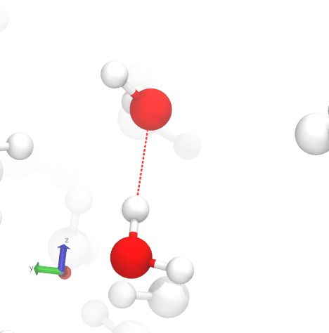
4

  FIG. 5. The processing flow of the H-bond configuration change classifier based on RNN. (i). Different types of h̃ sequences: T1 : Formation
  or no H-bond; T2 , T3 : No change; T4 : Negative sequence; T5 , T6 : Diffusion; T7 , T8 : interchange. We refer to the sequences of breakage
  and interchange as positive sequences. (ii). The preprocessor filters out the high-frequency components of h̃ and excludes T1 , T2 , and T3 .
  (iii). The classifier consists of a BLSTM AE to separate the positive and negative sequences and a final classifier to distinguish breakage and
  interchange sequences.

  Methods Section III C, Eq. 5). After training, the autoencoder                                nally, we use a final classifier to distinguish sequences be-
  can reconstruct positive processes very well. However, when                                   tween interchange and breakage processes from positive se-
  we input negative sequences into the AE, likely, it would not                                 quences. We use the range of a positive sequence x to deter-
  be able to reconstruct them well, leading to the reconstruc-                                  mine whether it is interchange or breakage, which is defined
  tion errors of these negative sequences greater than that of the                              as δ (x) = max x − min x.
  positive sequences. Through the reconstruction error, we can                                     Figure 6 (A) shows the densities of the reconstruction er-
  determine whether a h̃ sequence is positive or negative. Fi-                                  rors for interchange, breakage, and negative sequences. Since
                                                                                                BLSTM AE can reconstruct positive sequences well, the re-
          250 A                                                                  Interchange    construction errors of interchange and breakage sequences are
                                                                                 Breakage       small, most of which are smaller than the reconstruction er-
          200          =                                                         Negative
                            T                                                                   ror threshold LT (LT determination and corresponding accu-
          150
Density

                                                                                                racy analysis are described in SI Sec. 3, Fig. S3). Negative
          100                                                                                   sequences are not used to train the autoencoder, so it is much
                                                                                                more difficult to reconstruct them. Hence, the reconstruction
            50                                                                                  errors are relatively large, most of which are greater than LT .
             0
            0.000   0.025       0.050   0.075   0.100         0.125     0.150   0.175   0.200
                                                                                                As long as we find a suitable reconstruction error threshold,
                                                                                                we can get a classifier for positive and negative sequences.
            20 B                                                                 Interchange    Figure 6 (B) shows the densities for the range of normalized
                                                                                 Breakage       interchange and breakage sequences. The two distributions
            15                                  =   T                                           are significantly different from each other. Therefore, the final
  Density

                                                                                                classifier can distinguish interchange and breakage sequences
            10
                                                                                                very well via δT = 0.66, as shown in the dashed line (see the
            5                                                                                   classification process in SI Sec. 3, Fig. S4-S5 ). Therefore,
                                                                                                we have obtained an H-bond configuration change classifier
            0          0.4              0.6             0.8           1.0        1.2            based on an RNN autoencoder.

  FIG. 6. (A) Densities of reconstruction error L for interchange,                              D.   Proportions of interchange at different temperatures
  breakage, and negative sequences. (i) BLSTM AE can reconstruct
  positive sequences well. Hence, the reconstruction errors for inter-
  change and breakage sequences are relatively small, mainly less than                             To explore the effect of temperature on the H-bond config-
  LT . (ii) Since negative sequences are not used to train BLSTM                                uration change process, we have simulated nine bulk water
  AE, it is much more difficult for the autoencoder to reconstruct                              systems containing N = 64 water molecules. The tempera-
  them. Therefore, the reconstruction errors are relatively large, mainly                       ture ranges from 280 to 360 K every 10 K. Using the RNN-
  greater than LT . (iii) Once LT is determined, we use it as the thresh-                       based model, we classify h̃ sequence, count the number of
  old to distinguish positive and negative sequences. (B) Densities of                          interchange and breakage sequences at each temperature. As
  the range δ for interchange and breakage sequences. The two densi-                            shown in Fig. 7, the number of interchange and breakage pro-
  ties are significantly different from each other.                                             cesses shows a "rising first, then decreasing" trend as the tem-
5

         2000
                      A                                                                                           1635                          Interchange
                                                                                1518            1464                                            Breakage
         1500                                                      1375
                                                                                                                                    1126            1243
Number

         1000               811                            913
                                             771
            500                                                  332          340            313               355                                 273
                          154           206             184                                                                      168
                 0
                      B
                1.0                                                                                                                  87%
                            84%              79%           83%     81%          82%              82%               82%                                 82%
                0.8
   Percentage

                0.6
                0.4
                          16%           21%             17%      19%          18%           18%               18%                                 18%
                0.2                                                                                                             13%
                0.0        280              290           300     310         320         330                    340               350               360
                                                                          Temperature [K]
 FIG. 7. The number (A) and proportion (B) of interchange and breakage processes determined by the RNN-based classifier at different
 temperatures. (i) With the temperature increasing, the number of interchange and breakage processes increases first and then decreases on the
 whole. (ii) The relative ratio of interchange to breakage basically does not depend on temperature.

 perature increases. In other words, there is an overall upward                bond direction is ignored. The factor 2 is derived from the fact
 trend from 280 to 330 K. However, as the temperature contin-                  that one H-bond in water is shared by two water molecules.
 ues to rise, the number of detected interchange and breakage                  For a certain trajectory at one temperature, by counting nHB
 processes tends to decrease. As we use the method of width-                   at each time t, we get the distribution of nHB (one density
 fixed sliding window, the absolute number of interchanges and                 plot in Fig. 8 A). Then we use an L-dimensional vector h̃(t)
 breakages would change along the step size of sliding win-                    to represent the coarse-grained H-bond network configuration
 dow. These numbers would increase as we decrease the step                     for the simulated bulk water system at time t in Eq. 3,
 size. Therefore, we focused on the trend of the detected pro-
 cesses over the temperatures. On the other hand, although the                         h̃(t) = (h̃12 (t), h̃13 (t), · · · , h̃i j (t), · · · , h̃N−1,N (t))   (3)
 number of interchange and breakage processes vary at differ-
 ent temperatures, the relative ratios between the two are al-                 where L = N(N − 1)/2 is the number of Q-bonds in the sys-
 most unchanged, which is still about 1:4 (see SI Sec.4 for the                tem. So in a unit time, we get a set H of h̃(t) in Eq. 4,
 step size effect of the sliding window). This result indicates
 that the relative ratio is almost not dependent on temperature,                           H = {h̃(t) | t = t0 + k∆t, k = 0, 1, · · · , M}                    (4)
 and the interchange process is another important mechanism
                                                                               where t0 represents the start time of the unit time window, ∆t
 in bulk water besides the breakage process. Next, we will ex-
                                                                               is the time interval between two adjacent frames, and M is the
 plain this trend of the number of interchange and breakage
                                                                               length of the unit time window. In a unit time tw = M∆t, the
 processes from the following two aspects: the number of H-
                                                                               number of graph configuration can be expressed as Ω = |H|,
 bond per molecule and the change rate of the coarse-grained
                                                                               where |H| is the size of the set H, i.e., the number of different
 H-bond network configuration.
                                                                               h̃ vectors in this unit time. The number Ω of graph config-
                                                                               uration per unit time characterizes the rate of breakage and
 E.         The trend of interchange and breakage process number               reforming of the H-bonds in bulk water. The theoretical upper
                                                                               bound of Ω in tw is M + 1; in this case, all h̃ vectors are dif-
   To understand the trend in Fig. 7 (A), we first calculate the               ferent. By changing the start point t0 , we get the distribution
 number of H-bonds per molecule (nHB ) in the simulated sys-                   of Ω.
 tem. At time t, nHB can be expressed as Eq. 2,                                   Figure 8 shows the temperature dependence of the distribu-
                                                                               tions of nHB and ln Ω. The width of a density plot indicates the
                                            2 N N                              probability of nHB or ln Ω at the corresponding temperature.
                                nHB (t) =     ∑ ∑ |h̃i j (t)|
                                            N i=1
                                                                        (2)    From the medians (white dots) of violin plots in Fig. 8 (B), we
                                                  j>i
                                                                               see Ω is relatively smaller at lower temperatures, indicating
 where N = 64 is the number of water molecules in bulk water                   fewer changes of H-bond configuration in the unit time. This
 systems, and |h̃i j (t)| is the absolute value of h̃i j (t), i.e., the H-     result explains why the number of interchange and breakage
6

            A                                                           in the future.
      2.0

      1.5                                                               B.    Sequence collection and preprocessing
nHB

      1.0
                                                                             The sequence length of h̃ was 200 corresponding to 8 ps
      0.5                                                               simulation time. Positive sequences in which only one inter-
                                                                        change or breakage process occurred were collected. Nega-
                               Temperature [K]                          tive h̃ sequences used to evaluate the BLSTM AE classifier
      6.0 B                                                             were also collected. BLSTM AE was trained by 6786 positive
      5.8                                                               sequences, of which the interchange and breakage processes
      5.6                                                               each accounted for half (754 positive sequences at each tem-
      5.4
ln

                                                                        perature). There were 18,931 negative sequences for evalu-
      5.2                                                               ating the BLSTM AE classifier. The filtered sequence h̃ f [n]
      5.0                                                               was obtained by second-order Butterworth filter implemented
      4.8                                                               by Scipy55 . In addition, if h̃ f [0] − 0.5 < 0.15, indicating no
           280   290   300   310   320      330   340   350    360      H-bond at the beginning ( T1 ). If the standard deviation σ of
                               Temperature [K]                          h̃ f [n] satisfy σ < 0.1, then we consider the H-bond configura-
                                                                        tion in the Q-bond has not changed ( T2 , T3 ).
FIG. 8. The temperature dependence of (A) The distributions of
the number nHB of H-bonds per molecule. (B) The distributions of
ln Ω characterizing the rate of H-bond breakage and reforming. The
                                                                        C.    Bidirectional LSTM autoencoder classifier
dashed line denotes the upper bound of ln Ω in the unit time of 1 ps.

                                                                           The encoder and the decoder of BLSTM AE can be ex-
processes at lower temperatures in Fig. 7 (A) are smaller. Be-          pressed as two transformations, φ : X → F and ψ : F → X ,
sides, the direct reason for the decrease in the number of inter-       where X and F are the input space and the feature space,
change and breakage processes at higher temperatures is that            respectively. The dimension of F is smaller than that of
thermal motions tend to break H-bonds (thus reducing nHB ).             X , and the feature vector φ (x) is the compressed represen-
Therefore, the number of interchange and breakage processes             tation of input x. The input x of BLSTM AE is the nor-
in Fig. 7 (A) is determined by nHB and Ω together.                      malized and filtered directed H-bond population operator se-
                                                                        quence h̃ f [n]. The reconstruction error of BLSTM AE for a
                                                                        sequence x = h̃ f [n] is defined as
III.        METHODS
                                                                                         Lω,ω 0 (x) = kx − ψω 0 (φω (x))k2           (5)

A.      AIMD simulations                                                where ω, ω 0 represent the parameters of the encoder and de-
                                                                        coder respectively. The purpose of training is to obtain the
   AIMD simulations were carried out for bulk water of 64               optimal ω, ω 0 ,
water molecules within the canonical NVT ensemble us-
ing CP2K/QUICKSTEP (v7.1)47 . The number N of water                                                              1 m
                                                                                         ω ∗ , ω 0∗ = arg min0     ∑ Lω,ω 0 (xi )    (6)
molecules was 64 for all bulk water systems at different tem-                                            ω,ω     m i=1
peratures from 280 to 360 K. The length of the periodic cubic
box was 12.4295 Å. The discretized integration time step ∆t             where xi represents the i-th sequence (SI, Fig. S1-S2).
was set to 0.5 fs. The simulation time was 60 ps. The BLYP
functional, which consists of Becke non-local exchange48 and
Lee-Yang-Parr correlation49 , was used; Interactions between            IV.   SUMMARY
the valence electrons and the ionic cores were described by
GTH pseudopotentials50,51 ; Valence electrons were expanded                In summary, we have designed and trained a deep learning-
in a basis set consisting of double-zeta Gaussian functions52           based model to recognize different types of processes related
and plane waves with a cutoff energy of 280 Ry47 . The Nosé-           to H-bonds. The priority of this model are its remarkable abil-
Hoover chain thermostat53 was used to conserve temperature.             ity to classify different dynamic processes of water molecules
DFT-D3 correction54 for the dispersion interaction was used             and its wide range of applications to different kinds of simula-
to obtain a more accurate description of the vibrational prop-          tion methods. The model can be transfered to other dynamic
erties. It is worth mentioning that the analysis method we pro-         systems containning H-bonds with the form of O-H · · · O. As a
posed can be used on various simulation data, and the AIMD              feasible example, combined with AIMD simulations, we have
simulation used here is one of the options. The graph-based             found that the relative ratio of interchange and breakage pro-
analysis method is independent of simulation data, so this              cesses in bulk water is approximately 1:4, and this ratio hardly
method can be used to analyze more accurate simulation data             depends on temperature.
7
Moreover, the key concepts used in this work are the dy- 17 H. J. Bakker and H.-K. Nienhuys, “Delocalization of protons in liquid wa-
namic graph and the newly defined directed H-bond popu- ter,” Science 297, 587–590 (2002).
18 C. J. Fecko, “Ultrafast hydrogen-bond dynamics in the infrared spec-
lation. This reasonable coarse-grained description of the H-
troscopy of water,” Science 301, 1698–1702 (2003).
bond network simplifies the analysis of H-bond dynamics dra- 19 K. ichi Inoue, M. Ahmed, S. Nihonyanagi, and T. Tahara, “Reorientation-
matically. This work demonstrates that the semi-supervised induced relaxation of free OH at the air/water interface revealed by ultrafast
RNN-based model has an outstanding capability of classify- heterodyne-detected nonlinear spectroscopy,” Nature Communications 11
ing the dynamic processes related to H-bonds in bulk water, (2020), 10.1038/s41467-020-19143-8.
20 T. Iwashita, B. Wu, W.-R. Chen, S. Tsutsui, A. Q. R. Baron, and T. Egami,
which implies the great potential to extend our present scheme “Seeing real-space dynamics of liquid water through inelastic x-ray scatter-
to distinguish more complex dynamic processes in other sys- ing,” Science Advances 3, e1603079 (2017).
tems like the water-vapor interface and electrolyte solutions. 21 Z.-H. Loh, G. Doumy, C. Arnold, L. Kjellsson, S. H. Southworth, A. A.
Haddad, Y. Kumagai, M.-F. Tu, P. J. Ho, A. M. March, R. D. Schaller, M. S.
B. M. Yusof, T. Debnath, M. Simon, R. Welsch, L. Inhester, K. Khalili,
K. Nanda, A. I. Krylov, S. Moeller, G. Coslovich, J. Koralek, M. P. Minitti,
ACKNOWLEDGMENTS
W. F. Schlotter, J.-E. Rubensson, R. Santra, and L. Young, “Observation
of the fastest chemical processes in the radiolysis of water,” Science 367,
This research was supported by the National Natural Sci- 179–182 (2020).
22 T. Head-Gordon and G. Hura, “Water structure from scattering experiments
ence Foundation of China (NSFC) (Grant Nos. 21973070).
and simulation,” Chemical Reviews 102, 2651–2670 (2002).
The simulations were performed on the cluster in the College 23 V. A. Ranea, A. Michaelides, R. Ramírez, P. L. de Andres, J. A. Vergés,
of Mathematics and Physics at Wenzhou University. and D. A. King, “Water dimer diffusion on pd{111} assisted by an h-bond
1 D.
donor-acceptor tunneling exchange,” Physical Review Letters 92 (2004),
Kennedy, “What don’t we know?” Science 309, 75–75 (2005). 10.1103/physrevlett.92.136104.
2 F. Franks, Water: a matrix of life, 2nd ed. (Royal Society of Chemistry, 24 D. Laage and J. T. Hynes, “A Molecular Jump Mechanism of Water Reori-
2000). entation,” Science 311, 832–835 (2006).
3 S. K. Pal and A. H. Zewail, “Dynamics of water in biological recognition,”
25 W. Fang, J. Chen, P. Pedevilla, X.-Z. Li, J. O. Richardson, and
Chemical Reviews 104, 2099–2124 (2004). A. Michaelides, “Origins of fast diffusion of water dimers on surfaces,”
4 M. Chaplin, “Do we underestimate the importance of water in cell biol-
Nature Communications 11 (2020), 10.1038/s41467-020-15377-8.
ogy?” Nature Reviews Molecular Cell Biology 7, 861–866 (2006). 26 F. N. Keutsch and R. J. Saykally, “Water clusters: Untangling the mysteries
5 P. Ball, “Water is an active matrix of life for cell and molecular biol-
of the liquid, one molecule at a time,” Proceedings of the National Academy
ogy,” Proceedings of the National Academy of Sciences 114, 13327–13335 of Sciences 98, 10533–10540 (2001).
(2017). 27 R. S. Fellers, C. Leforestier, L. B. Braly, M. G. Brown, and R. J. Saykally,
6 F. H. Stillinger, “Water revisited,” Science 209, 451–457 (1980).
7 J. R. Errington and P. G. Debenedetti, “Relationship between structural or-
“Spectroscopic determination of the water pair potential,” Science 284,
945–948 (1999).
der and the anomalies of liquid water,” Nature 409, 318–321 (2001). 28 N. Agmon, “The grotthuss mechanism,” Chemical Physics Letters 244,
8 I. Dumé, “Second critical point appears in two models of water,” Physics
456–462 (1995).
World 33, 7i–7i (2020). 29 J. L. Thomaston, R. A. Woldeyes, T. Nakane, A. Yamashita, T. Tanaka,
9 R. Kumar, J. R. Schmidt, and J. L. Skinner, “Hydrogen bonding defini-
K. Koiwai, A. S. Brewster, B. A. Barad, Y. Chen, T. Lemmin, M. Uerviro-
tions and dynamics in liquid water,” The Journal of Chemical Physics 126, jnangkoorn, T. Arima, J. Kobayashi, T. Masuda, M. Suzuki, M. Sugahara,
204107 (2007). N. K. Sauter, R. Tanaka, O. Nureki, K. Tono, Y. Joti, E. Nango, S. Iwata,
10 A. Nilsson and L. G. M. Pettersson, “The structural origin of anoma-
F. Yumoto, J. S. Fraser, and W. F. DeGrado, “XFEL structures of the in-
lous properties of liquid water,” Nature Communications 6 (2015), fluenza m2 proton channel: Room temperature water networks and insights
10.1038/ncomms9998. into proton conduction,” Proceedings of the National Academy of Sciences
11 U. Wilhelmsen and D. Deutsches Elektronen-Synchrotron, The strangest
114, 13357–13362 (2017).
liquid in the world: water amazes scientists time and again, edited by 30 M. D. Gelenter, V. S. Mandala, M. J. M. Niesen, D. A. Sharon, A. J. Dregni,
T. Mundzeck, Vol. 20 (Deutsches Elektronen Synchrotron, DESY, Ham- A. P. Willard, and M. Hong, “Water orientation and dynamics in the closed
burg, 2020) p. 44 pages. and open influenza b virus m2 proton channels,” Communications Biology
12 E. T. Karamatskos, S. Raabe, T. Mullins, A. Trabattoni, P. Stammer,
4, 338 (2021).
G. Goldsztejn, R. R. Johansen, K. Długołecki, H. Stapelfeldt, M. J. J. 31 T. D. Kühne, M. Iannuzzi, M. D. Ben, V. V. Rybkin, P. Seewald, F. Stein,
Vrakking, S. Trippel, A. Rouzée, and J. Küpper, “Molecular movie of ul- T. Laino, R. Z. Khaliullin, O. Schütt, F. Schiffmann, D. Golze, J. Wilhelm,
trafast coherent rotational dynamics of OCS,” Nature Communications 10 S. Chulkov, M. H. Bani-Hashemian, V. Weber, U. Borštnik, M. Taille-
(2019), 10.1038/s41467-019-11122-y. fumier, A. S. Jakobovits, A. Lazzaro, H. Pabst, T. Müller, R. Schade,
13 F. Perakis, G. Camisasca, T. J. Lane, A. Späh, K. T. Wikfeldt, J. A. Sell-
M. Guidon, S. Andermatt, N. Holmberg, G. K. Schenter, A. Hehn,
berg, F. Lehmkühler, H. Pathak, K. H. Kim, K. Amann-Winkel, S. Schreck, A. Bussy, F. Belleflamme, G. Tabacchi, A. Glöß, M. Lass, I. Bethune, C. J.
S. Song, T. Sato, M. Sikorski, A. Eilert, T. McQueen, H. Ogasawara, Mundy, C. Plessl, M. Watkins, J. VandeVondele, M. Krack, and J. Hutter,
D. Nordlund, W. Roseker, J. Koralek, S. Nelson, P. Hart, R. Alonso-Mori, “CP2k: An electronic structure and molecular dynamics software package
Y. Feng, D. Zhu, A. Robert, G. Grübel, L. G. M. Pettersson, and A. Nils- - quickstep: Efficient and accurate electronic structure calculations,” The
son, “Coherent x-rays reveal the influence of cage effects on ultrafast water Journal of Chemical Physics 152, 194103 (2020).
dynamics,” Nature Communications 9 (2018), 10.1038/s41467-018-04330- 32 D. E. Moilanen, D. Wong, D. E. Rosenfeld, E. E. Fenn, and M. D. Fayer,
5. “Ion–water hydrogen-bond switching observed with 2d ir vibrational echo
14 T. Mitsui, “Water diffusion and clustering on pd(111),” Science 297, 1850–
chemical exchange spectroscopy,” Proceedings of the National Academy of
1852 (2002). Sciences 106, 375–380 (2009).
15 T. Kumagai, M. Kaizu, S. Hatta, H. Okuyama, T. Aruga, I. Hamada, and
33 M. Ji, M. Odelius, and K. J. Gaffney, “Large angular jump mechanism ob-
Y. Morikawa, “Direct observation of hydrogen-bond exchange within a served for hydrogen bond exchange in aqueous perchlorate solution,” Sci-
single water dimer,” Physical Review Letters 100 (2008), 10.1103/phys- ence 328, 1003–1005 (2010).
revlett.100.166101. 34 R. Schulz, Y. von Hansen, J. O. Daldrop, J. Kappler, F. Noé, and R. R.
16 S. Woutersen, U. Emmerichs, and H. J. Bakker, “Femtosec- Netz, “Collective hydrogen-bond rearrangement dynamics in liquid water,”
ond mid-ir pump-probe spectroscopy of liquid water: Evidence The Journal of Chemical Physics 149, 244504 (2018).
for a two-component structure,” Science 278, 658–660 (1997), 35 N. R. Samala and N. Agmon, “Thermally induced hydrogen-bond rear-
https://science.sciencemag.org/content/278/5338/658.full.pdf.8 rangements in small water clusters and the persistent water tetramer,” ACS Computation 9, 1735–1780 (1997). Omega 4, 22581–22590 (2019). 47 J. VandeVondele, M. Krack, F. Mohamed, M. Parrinello, T. Chassaing, and 36 E. Méndez and D. Laria, “Nuclear quantum effects on the hydrogen bond J. Hutter, “Quickstep: Fast and accurate density functional calculations us- donor–acceptor exchange in water–water and water–methanol dimers,” The ing a mixed gaussian and plane waves approach,” Comput. Phys. Commun. Journal of Chemical Physics 153, 054302 (2020). 167, 103–128 (2005). 37 A. Luzar and D. Chandler, “Hydrogen-bond kinetics in liquid water,” Na- 48 A. D. Becke, “Density-functional exchange-energy approximation with ture 379, 55–57 (1996). correct asymptotic behavior,” Phys. Rev. A 38, 3098 (1988). 38 F. Sciortino and S. L. Fornili, “Hydrogen bond cooperativity in simulated 49 C. Lee, W. Yang, and R. G. Parr, “Development of the colic-salvetti water: Time dependence analysis of pair interactions,” The Journal of correlation-energy formula into a functional of the electron density,” Phys. Chemical Physics 90, 2786–2792 (1989). Rev. B 37, 785 (1988). 39 S. Balasubramanian, S. Pal, and B. Bagchi, “Hydrogen-bond dynamics 50 C. Hartwigsen, S. Goedecker, and J. Hutter, “Relativistic separable dual- near a micellar surface: Origin of the universal slow relaxation at com- space gaussian pseudopotentials from H to Rn,” Phys. Rev. B 58, 3641– plex aqueous interfaces,” Physical Review Letters 89 (2002), 10.1103/phys- 3662 (1998). revlett.89.115505. 51 J. H. G. Lippert and M. Parrinello, “The gaussian and augmented-plane- 40 N. Michaud-Agrawal, E. J. Denning, T. B. Woolf, and O. Beckstein, “MD- wave density functional method for ab initio molecular dynamics simula- Analysis: A toolkit for the analysis of molecular dynamics simulations,” tions,” Theor. Chem. Acc. 103, 124 (1999). Journal of Computational Chemistry 32, 2319–2327 (2011). 52 J. VandeVondele and J. Hutter, “Gaussian basis sets for accurate calcula- 41 M. G. Brown, F. N. Keutsch, and R. J. Saykally, “The bifurcation rear- tions on molecular systems in gas and condensed phases,” The Journal of rangement in cyclic water clusters: Breaking and making hydrogen bonds,” Chemical Physics 127, 114105 (2007). The Journal of Chemical Physics 109, 9645–9647 (1998). 53 G. J. Martyna, M. L. Klein, and M. Tuckerman, “Nosé-hoover chains: The 42 T. W. Hughes, I. A. D. Williamson, M. Minkov, and S. Fan, “Wave canonical ensemble via continuous dynamics,” J. Chem. Phys. 97, 2635 physics as an analog recurrent neural network,” Science Advances 5 (2019), (1992). 10.1126/sciadv.aay6946. 54 S. Grimme, J. Antony, S. Ehrlich, and H. Krieg, “A Consistent and Accu- 43 N. Rank, B. Pfahringer, J. Kempfert, C. Stamm, T. Kühne, F. Schoenrath, rate Ab Initio Parametrization of Density Functional Dispersion Correction V. Falk, C. Eickhoff, and A. Meyer, “Deep-learning-based real-time pre- (DFT-D) for the 94 Elements H-Pu,” J. Chem. Phys. 132, 154104 (2010). diction of acute kidney injury outperforms human predictive performance,” 55 P. Virtanen, , R. Gommers, T. E. Oliphant, M. Haberland, T. Reddy, npj Digital Medicine 3 (2020), 10.1038/s41746-020-00346-8. D. Cournapeau, E. Burovski, P. Peterson, W. Weckesser, J. Bright, S. J. 44 S.-T. Tsai, E.-J. Kuo, and P. Tiwary, “Learning molecular dynamics with van der Walt, M. Brett, J. Wilson, K. J. Millman, N. Mayorov, A. R. J. simple language model built upon long short-term memory neural net- Nelson, E. Jones, R. Kern, E. Larson, C. J. Carey, İ. Polat, Y. Feng, E. W. work,” Nature Communications 11 (2020), 10.1038/s41467-020-18959-8. Moore, J. VanderPlas, D. Laxalde, J. Perktold, R. Cimrman, I. Henriksen, 45 J. J. Hopfield, “Neural networks and physical systems with emergent col- E. A. Quintero, C. R. Harris, A. M. Archibald, A. H. Ribeiro, F. Pedregosa, lective computational abilities,” Proceedings of the National Academy of and P. van Mulbregt, “SciPy 1.0: fundamental algorithms for scientific com- Sciences 79, 2554–2558 (1982). puting in python,” Nature Methods 17, 261–272 (2020). 46 S. Hochreiter and J. Schmidhuber, “Long short-term memory,” Neural
You can also read