Investigating the Influences of Tree Coverage and Road Density on Property Crime - MDPI
←
→
Page content transcription
If your browser does not render page correctly, please read the page content below
International Journal of
           Geo-Information

Article
Investigating the Influences of Tree Coverage and
Road Density on Property Crime
Chengming Ye 1,2        ID
                             , Yifei Chen 2 and Jonathan Li 2, *   ID

 1    Key Laboratory of Earth Exploration and Information Technology of Ministry of Education,
      Chengdu University of Technology, Chengdu 610059, China; rsgis@sina.com
 2    Mobile Sensing and Geodata Science Lab, Department of Geography and Environmental Management,
      University of Waterloo, 200 University Ave West, Waterloo, ON N2L 3G1, Canada; y378chen@uwaterloo.ca
 *    Correspondence: junli@uwaterloo.ca

 Received: 22 December 2017; Accepted: 12 March 2018; Published: 14 March 2018

 Abstract: With the development of Geographic Information Systems (GIS), crime mapping has
 become an effective approach for investigating the spatial pattern of crime in a defined area.
 Understanding the relationship between crime and its surrounding environment reveals possible
 strategies for reducing crime in a neighborhood. The relationship between vegetation density and
 crime has long been under debate. The convenience of a road network is another important factor
 that can influence a criminal’s selection of locations. This research is conducted to investigate
 the correlations between tree coverage and property crime, and road density and property crime
 in the City of Vancouver. High spatial resolution airborne LiDAR data and road network data
 collected in 2013 were used to extract tree covered areas for cross-sectional analysis. The independent
 variables were inserted into Ordinary Least-Squares (OLS) regression, Spatial Lag regression, and
 Geographically Weighted Regression (GWR) models to examine their relationships to property crime
 rates. The results of the cross-sectional analysis provide statistical evidence that there are negative
 correlations between property crime rates and both tree coverage and road density, with the stronger
 correlations occurring around Downtown Vancouver.

 Keywords: crime mapping; GIS; urban vegetation; road density; spatial lag; geographically
 weighted regression

1. Introduction
      The global trend toward urbanization has driven urban sprawl in most metropolitan areas around
the world. Thus, effective urban design strategies are required to provide citizens a prosperous,
sustainable and safe living environment. To ensure the safety of residents, crime prevention has always
been a crucial part of urban planning. The study and analysis of crime focus mainly on these two
aspects: who are the persons that commit crime, and at what places do crimes occur [1]. Regarding the
first aspect, the great complex and diverse nature of human thinking can be an obstacle to analysis and
control. Thus, to discover crime patterns, geography researchers focus on when and where crimes
occur. As Ferreira et al. [2] summarized, since the 1960s, Geographic Information Systems (GIS) have
been applied to a number of studies; meanwhile, digital crime mapping, developed significantly in the
1980s, has been widely applied to the criminology field. GIS technologies have been used in various
ways including, but not limited to, monitoring alerts reported by citizens, providing visual aids for
identifying crime distribution patterns, and identifying, modeling and predicting crime “hotspots”.
Additionally, web mapping enables researchers, as well as the public, to obtain volunteer provided
information for crime analysis and prevention.
      Since the mid-nineteenth century, crime pattern studies, whether using paper or digital maps, have
revealed, from a place perspective, that criminal activity is highly patterned, and thus, predictable [3]

ISPRS Int. J. Geo-Inf. 2018, 7, 101; doi:10.3390/ijgi7030101                     www.mdpi.com/journal/ijgi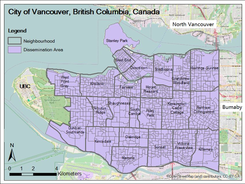
ISPRS Int. J. Geo-Inf. 2018, 7, 101                                                                  2 of 14

In other words, incidents of crime are not randomly spatially distributed; crime “hotspots” do exist [4].
Researchers also found that the “hotspots” are stable year after year [5], thus suggesting that we can
deal with crime problems by concentrating on the identified hotspots, which are within a small number
of places. Based on the fact that the distribution of the incidents of crime follows a pattern, the concept
of Crime Prevention Through Environmental Design (CPTED) has been proposed since the 1970s,
which asserts that “the proper design and effective use of a built environment can lead to a reduction
in the fear and incidence of crime and an improvement in the quality of life” [6]. Discovering the
characteristics of crime-concentrated places supports the planning of CPTED strategies. Empirical
models are developed to summarize characteristics. Accordingly, predictive models are built to predict
high-risk crime areas [7–9].
      Factors that affect crime rates. Various factors, including population density, poverty level, and
the unemployment rate affect crime rates [5]. The important factor most often included in crime
research is population density. Although exhibiting different effects (positive or negative), population
density is highly significant when predicting crime [10–14]. Shaw and McKay [15] introduced a social
disorganization theory that suggests poverty, ethnic heterogeneity, and residential mobility are the three
ecological predictors of crime, which promote crime by increasing social disorganization. Subsequent
research has added several other factors to the list, including lone-parent families, structural density,
urbanization, etc. [16]. According to crime studies, most types of crime are positively related to
the poverty level [1,12]. Troy et al. [11], in their analysis, showed that the relationship between the
percentage of single-parent families and crime is negative; whereas, in other regions, its influence is
still uncertain. Wang and Minor [17] found a strong negative relationship between employment and
crime in Cleveland in 1990, and the effect on economic crimes was greater than the effect on violent
crimes. A study [10] conducted in Vancouver showed similar results. Also, researchers have examined
the influences of educational attainment and a young population. Studies of crime and physical
environment mostly focus on the presence, or absence, of structures, such as commercial buildings,
parking lots, police stations, bus stops, etc. [5,18]. The number of street lights in prosperous regions,
which provide more opportunities for property crime, serve as an indicator of the urbanization level
of an area [9]. The criminology of place study in Seattle [5] revealed a positive relationship between
lighting and crime. Riggs [19] also suggested that street lights make it easier for criminals to see the
contents of parked cars when stealing, or to make sure there is no one around when breaking into a
house. Urban layout has also proved to be related to crime [14]. The above factors have already shown
they have an impact on crime. However, the following are also potential influential factors that can
add to accuracy when predicting crime.
      Relationship between vegetation density and crime. The relationship between vegetation
density and crime has long been under debate. Studies find that criminals usually use dense vegetation
as a shield when committing crimes; therefore, vegetation is positively related to the incidents of
crime [20]. On the other hand, some studies indicate that vegetation is related to a decrease in crime
incidents. One of the possible reasons is that the green spaces attract people to spend time outdoors,
thereby creating a natural surveillance around the area [11,21]. Providing A further reason comes from
the attention restoration theory, which suggests that the mentally restorative effect of the vegetation
may reduce violent crimes by restraining the psychological precursors to criminal acts [12,21,22].
Another possible explanation is related to the broken windows theory, which suggests that the green
spaces in an urban area indicate a well-managed society that creates an atmosphere of order and
lawfulness, thereby preventing crime from occurring [22].
      Convenience of road networks. The convenience of road networks is another important factor
that can influence a criminal’s selection of locations. Highly accessible areas are associated with
higher property crime rates; whereas, complex road networks reduce this type of crime [23]. This
phenomenon can be explained by the routine activities theory that the convenient road network
exposes attractive and unguarded targets to potential criminals. In addition, higher traffic flows create
a natural surveillance that can reduce the crime rate to some extent [23].
ISPRS Int. J. Geo-Inf. 2018, 7, 101 3 of 14
Studies conducted to discover the relationship between vegetation and crime in Canadian cities
are limited. Likewise, few studies concerning the relationship between road networks and crime in
Canada are documented. Urban crime is usually categorized by violent crime, also known as crime
against persons. Non-violent crime is known as crime against property. Based on the available data,
the purpose of our study is to discover the statistical relationships between urban property crime and
high-vegetation coverage and urban property crime and road network density in the city of Vancouver.
Types of non-violent property crimes, including breaking and entering (BNE), theft, and mischief, were
analyzed. The objectives of our study are as follows: (1) to understand the spatial patterns of property
crime; (2) to understand the spatial relationships between tree coverage and property crime, as well as
road density and property crime; (3) to explore the spatial variation of the correlations between the two
factors and property crime; and (4) to support decision making in urban property crime prevention
and reduction strategies.
2. Literature Review
Various studies have been performed to examine the physical and social environment around
crime hotspots. In terms of the surrounding physical environment, the presence of the following
are found to be related to the concentration of crime: parking lots, commercial buildings, facilities
(e.g., bus stops, police stations, street lighting, etc.), urban layout, and graffiti. However, few studies
examined the effect of vegetation. In some of the studies, the presence of vegetation and buildings was
used as an indicator to classify the land use of the study area [18,24,25]. According to Chen et al. [18],
the percentage of non-vegetated areas increases the accuracy of predicting crime hotspots and is
directly related to the occurrence of crime.
Relationship between vegetation and crime in U.S. cities. A few studies, most of which were
conducted in the United States, concentrated on identifying the relationship between vegetation and
crime. To understand the relationships among urban green space, violence, and crime in the U.S., Bogar
and Beyer [26] reviewed ten studies from 2001 to 2013. They found that the study methodology varies,
and so do the results; thus, they suggested standardization in design and measurement. The most
recent related studies are as follows:
Houston, TX and Philadelphia, PA. In their study of eleven community gardens and surrounding
areas in Houston, TX, Gorham et al. [27] compared the number of crime incidents in 2005 in the areas
surrounding the gardens with randomly selected areas in the city. Results showed no significant
difference between the number of property crimes in the areas surrounding the community gardens
and other areas in the city. In other words, the community gardens, studied in Houston, do not have
a strong effect on property crime. Garvin et al. [21] evaluated the influence of green space on crime
by conducting an experiment in Philadelphia, PA. The results of comparing the crime rate before and
after the greening of chosen vacant lots suggested a reduction in crime, but this was not significantly
related to the greening. However, the greening of vacant land does significantly increase the sense of
security of the residents.
Baltimore, MD; Philadelphia, PA; Portland, OR; Minneapolis, MN. Troy et al. [11] conducted a
study in the greater Baltimore region, including Baltimore City and Baltimore County, MD. Their study
took into account the different effects on crime of trees located in public or private land. Their analysis
shows a reverse relationship between crime rate (robbery, burglary and shooting) and vegetation
density. Roughly a twenty percent decrease in crime is expected when there is a ten percent increase in
tree cover. Also, there is evidence that the effect of tree canopies varies between public and private land.
Planting trees on public land results in higher crime-reduction benefits. However, in some areas there
is a direct relationship between trees and crime, probably because the trees are mostly unmanaged,
providing concealment for criminals. In a study performed in Philadelphia, Wolfe and Mennis [12]
conducted a spatial analysis of crime at the census tract level with similar results. The results indicate
that robberies, burglaries and assaults are inversely related to vegetation coverage. Also, Wolfe and
Mennis [12] found that vegetation has a greater negative effect on assault than on other types ofISPRS Int. J. Geo-Inf. 2018, 7, 101 4 of 14
crimes. However, there is no significant association between thefts and vegetation coverage. According
to Donovan and Prestemon [22], in Portland, Oregon, the crown area of street trees demonstrates
a negative effect on crime; whereas, the number of trees on the lot of a house is associated with
an increase in crime. Eckerson [13] found a negative relationship between vegetation and crime in
Minneapolis, MN.
Relationship between vegetation and crime in Canadian cities. There is limited research
examining the influence of vegetation on crime in Canadian cities. The most recent investigation
applies Ordinary Least-Squares (OLS) and Spatial Lag models to different crime types in the
Kitchener-Waterloo region, Ontario, [28]. The results indicate a negative correlation between crime
(both violent and non-violent) and vegetation density. A dissemination area, a standard geographic
unit with census data and small enough to provide a large sample size, was used for the unit of
analysis. Using Geographically Weighted Regression (GWR), Du [28] also examined the spatial
variation of the impacts from the two variables. However, Landsat imagery with a 30-m resolution is
too coarse to capture the detailed spatial variations in vegetation [29]. Moreover, the calculation of the
Normalized Difference Vegetation Index (NDVI) does not separate trees and grass, which may affect
crime differently.
Influence of road network on crime. Road network, which is less influential on crimes against
persons, primarily influences property crime. Road network complexity may reduce property crime
because criminals who are unfamiliar with an area may spend more time finding an escape route;
the convenience of a road network, however, provides criminals opportunities to acquire suitable
targets. Beavon et al. [23], who concluded that the property crime rate is higher in more accessible
and highly used areas, also suggested that traffic barriers and road closures can be used as potential
effective crime prevention techniques by reducing accessibility. Copes [30] performed a statistical
analysis, which demonstrates that road density (calculated by dividing the number of roads passing
through a tract by the area of the tract) directly influences the increase in motor vehicle theft. Copes’
results support the Beavon et al. [23] study that the routine activity of a criminal is associated with the
rate of property crime in an area, and road network is one of the methods to quantify the issue.
The relationship between road network patterns and crime has been analyzed in a few recent
studies. A study, conducted in Tokyo, Japan, by Murakami et al. [31], investigated the pattern of the
road network around five robbed convenience stores. Murakami et al. [31] found similarities in the
road environment of the five crime scenes. However, their result is not convincing because of the small
sample size, and, due to the absence of a control group, they failed to distinguish the characteristics
from other road environments. Foster et al. [32] conducted a survey in Perth, Australia that shows an
inverse relationship between a perceived crime risk and the street connectivity of the area, represented
by the number of three-way intersections. In other words, street connectivity actually increases the
residents’ perception of safety within the area.
The study conducted in the Kitchener-Waterloo region [28] also looked at the relationship between
road network and crime. Du [28] used road density as an explanatory variable in the crime regression
models and concluded there is a positive correlation between crime and road density. Also, the impact
is greater in the urban center of the region.
The number of studies on this topic is limited, and the results are restricted to the studied areas.
To understand the impact of road networks on crime in a particular area, research must be performed
using local data.
In summary, there has been extensive research conducted on crime spatial analysis. However,
there is insufficient insight into how crime and vegetation/road networks are related. Research is
inconsistently designed and focuses on particular cities or regions, thus providing a limited perspective
on the impact that vegetation and road networks have on crime.ISPRS Int. J. Geo-Inf. 2018, 7, 101 5 of 14
3. Methodology
3.1. Study Area
The City of Vancouver is a coastal city located on the southwest corner of British Columbia. Home
to 603,502 residents in 2011, Vancouver is the eighth largest Canadian municipality and the 5most
ISPRS Int. J. Geo-Inf. 2018, 7, x FOR PEER REVIEW of 14
populous city in Western Canada [33]. Although voted the most livable city in the world, Vancouver
has a high crime
Vancouver has arate
highand a high
crime rateCrime
and a Severity
high Crime Index (CSI), both
Severity Indexof(CSI),
whichbothare among
of whichtheare
topamong
ten in the
the
country [34,35]. This has drawn the attention of the public and scientists. To support
top ten in the country [34,35]. This has drawn the attention of the public and scientists. To support crime prevention
planning, various types
crime prevention of research
planning, varioushave beenofconducted.
types Also, to
research have enhance
been community
conducted. Also,awareness
to enhance of
crime, the Vancouver
community awarenessPolice Department
of crime, (VPD) recently
the Vancouver launched a (VPD)
Police Department Web-GIS application
recently launched (GeoDash),
a Web-
which shows the(GeoDash),
GIS application crime incidentswhich in shows
the city.the
Forcrime
Vancouver citizens
incidents to city.
in the viewForthe Vancouver
most up to date crime
citizens to
data, the
view the most
map is upupdated
to date every
crime business
data, the day
map[36].
is updated every business day [36].
Figure 11 shows
Figure shows the the study
study area
area and
and the
the local
local neighborhood
neighborhood boundaries.
boundaries. The The city
city is
is divided
divided into
into
dissemination areas (DA). DA is the smallest standard geographic unit, usually
dissemination areas (DA). DA is the smallest standard geographic unit, usually with a population of with a population of
400 to
400 to 700
700 persons
persons (Canadian
(Canadian Census
Census Program).
Program). As As of
of 2011,
2011, the
the City
City of
of Vancouver
Vancouver has
has 995
995 DAs,
DAs, which
which
give the regression analysis a sample size
give the regression analysis a sample size of N = 995. of N = 995.
Figure 1. Study area divided into dissemination areas: City of Vancouver, British Columbia.
Figure 1. Study area divided into dissemination areas: City of Vancouver, British Columbia.
3.2. Data and Geoprocessing
3.2. Data and Geoprocessing
Vancouver property crime data was obtained from the City of Vancouver Open Data catalogue,
Vancouver property crime data was obtained from the City of Vancouver Open Data catalogue,
which provides free access to the city’s datasets. The original tabular data, dating back to 2003, was
which provides free access to the city’s datasets. The original tabular data, dating back to 2003, was
provided by the VPD. Since the publishing of the GeoDash web application in 2015, the geocoded
provided by the VPD. Since the publishing of the GeoDash web application in 2015, the geocoded ESRI
ESRI point shapefiles are also available to the public from the Vancouver Open Data catalogue. The
point shapefiles are also available to the public from the Vancouver Open Data catalogue. The datasets
datasets provide information including crime type, year, month, neighborhood, and coordinates. In
provide information including crime type, year, month, neighborhood, and coordinates. In our study,
our study, BNE commercial and BNE residential/other are categorized as BNE; thefts from vehicles,
thefts of vehicles, and other thefts are categorized as theft. Property crime includes theft, BNE, and
mischief. For protection of privacy, violent types of crimes, including homicides and other crimes
against persons, have been excluded from the shapefiles. It should be noted that, according to the
VPD, for privacy and investigation purposes, the data does not include all the cases reported to theISPRS Int. J. Geo-Inf. 2018, 7, 101 6 of 14
BNE commercial and BNE residential/other are categorized as BNE; thefts from vehicles, thefts of
vehicles, and other thefts are categorized as theft. Property crime includes theft, BNE, and mischief.
For protection of privacy, violent types of crimes, including homicides and other crimes against
persons, have been excluded from the shapefiles. It should be noted that, according to the VPD, for
privacy and investigation purposes, the data does not include all the cases reported to the police. Also,
for privacy considerations, the coordinates of the crime incidents are offset from the actual crime scenes.
As the VPD states in their legal disclaimer: “for property related offences, the VPD has provided the
location to the hundred block of these incidents within the general area of the block.” [37]. In addition,
because victims may choose not to file a police report, the recorded cases do not necessarily include all
criminal activities. In our study, the 2013 crime rates of theft, BNE, and total property crime are the
three outcome variables defined as the ratio of the volume of crime in an area to the population of that
area, expressed as number of crimes per 1000 population per year.
High resolution tree crowns. High resolution tree crown area data was extracted from airborne
Light Detection and Ranging (LiDAR) data of Vancouver, collected in February 2013. The datasets
are in LAS file format and also openly available from the City of Vancouver Open Data catalogue,
provided by their GIS and CADD services branch. Because of the large size of the LiDAR point cloud,
the dataset was divided into 168 tiles covering the jurisdiction of the city. The density of the LiDAR
data is, on the average, 12 points/m2 , reaching a vertical accuracy of 18 cm and a horizontal accuracy
of 36 cm, both with a 95% confidence level. Selected points, representing tree crowns, were aggregated
into polygons. An assessment of accuracy was conducted for the derived tree covered areas. Vancouver
Orthophoto 2013 was used as the ground truth map. The region of interest (ROI) was selected based
on whether or not the area is covered by tree crowns. More than one million random pixels (7.5 cm
× 7.5 cm) were selected for comparison with the tree canopy polygons extracted from the LiDAR
data. Another one million pixels were selected from the land area that was not covered by tree crowns.
Because the extracted tree cover and ROI files were both polygon shapefiles, areas of the polygons
were calculated and an error matrix built accordingly. This error matrix was used to estimate user and
producer accuracy and overall accuracy of the tree canopy extraction.
Road network data. The 2013 road network data was obtained from Statistic Canada and applied
to the study area. Road density was calculated as the ratio of the sum of the road lengths to the land area.
The analysis also included population density, unemployment rate, percentage of lone-parent families,
percentage of low income families, number of street lights, and number of graffiti as ancillary data.
Census data of 2011 by dissemination area, including DA boundaries, was obtained from Statistics
Canada [33]. Point shapefiles, presenting the most up-to-date locations of every street light and graffiti,
were provided by Vancouver Open Data catalog and downloaded in 2015. The 2011 education and
labour data by DA was missing; the 2006 census data was used instead. Table 1 shows the description
and statistics of the variables.
Table 1. Variables descriptions.
Dependent Variables Description Min. Max. Mean STDV
PropertyCrimeRate Property crime rate per 1000 population by DA 0 1.44 × 10⁵ 4.87 × 10³ 8.33 × 10³
TheftCrimeRate Theft rate per 1000 population by DA 0 1.23 × 10³ 33.61 68.51
BNE BNE rate per 1000 population by DA 0 87.17 7.91 7.65
TreeCoverage Percent tree cover by DA 0.33 65.08 14.97 7.56
RoadDensity Road density (total length per 100 m2 ) by DA 0.14 4.44 2.32 0.51
PopDens Population density per 1000 m2 by DA 0.19 75.29 9.59 9.21
Unemplm06 2006 Unemployment rate (%) by DA 0 20.25 5.84 2.44
LowInc Percent of low income families by DA 0 92.11 19.87 12.43
LoneParent Percent of lone parent families by DA 0 42.86 6.95 8.19
LightDens Number of lights per 10,000 m2 by DA 0 29 6.04 4.54
Graffiti Number of graffiti per 10,000 m2 by DA 0 100.49 3.20 3.23ISPRS Int. J. Geo-Inf. 2018, 7, 101 7 of 14
3.3. Regression Models
According to previous crime studies, crimes usually have positive spatial autocorrelation;
locations with high crime rates are usually clustered. Statistical tests, taking the crime rates of
nearby DAs into account, were required to prove the presence of spatial autocorrelation of the
dependent variables. The global Moran’s I plots were generated using GeoDash; the Moran’s I
statistics of theft rate, BNE rate, and property crime rate were 0.44, 0.36, and 0.46, respectively, all with
a significance level of 0.001. The three positive values indicate the presence of spatial autocorrelation
of the examined variables.
The statistical relationships between crime and tree covered areas was assessed in the GeoDash
software using regression models. The OLS estimation was firstly applied to the examined types of
crimes, with all the dependent variables as covariates. However, as shown in the spatial autocorrelation
test results, the dependent variables are spatially autocorrelated. Using the OLS linear regression
model, which ignores the spatial autocorrelation of crime data, can lead to erroneous results. Therefore,
a spatial lag model was applied. More increase in the log likelihood of spatial regression model than
that of the OLS model suggest an improvement of fit of the data [38].
A spatial lag model, which is a spatial autoregressive model, assumes that the spatial
autoregressive process occurs only in the dependent variable [39] and is expressed in matrix notation
as follows [39,40]:
y = ρWy + Xβ + ε (1)
where, y is the dependent variable, X is a matrix of covariates, ρ and β are vectors of coefficients, ε is
an error term, and W is the spatial weights matrix. Geographically Weighted Regression (GWR) was
also employed in the ArcGIS platform to test for spatial non-stationarity and to investigate the local
regressions for crime in the Vancouver DAs. GWR is expressed as follows [40]:
yi = β0 (ui , vi ) + Σ βk (ui , vi ) xik + εi (2)
where β0 is a constant, (ui , vi ) stands for the coordinates of the ith regression “point”, βk is the kth
coefficient, xik is the kth independent variable for the ith observation, and εi is the ith error term.
GWR was applied to the three models in the ArcGIS platform. The performance of a model was
examined by comparing the AICc(Akaike Information Criterion with a correction for small sample
sizes) statistic with that of the corresponding OLS regression. A lower AICc value indicates a better fit
of the data [41]. GWR creates regressions that vary depending on the locations of the observations;
therefore, each observation has its local coefficient for each covariate [40]. Local coefficient maps,
where the local coefficients of the percentage of tree cover or road density are represented by symbols,
show the spatial distribution of the extent of impact from the two examined explanatory variables on
crime. The relatively insignificant coefficients (calculated as the ratio of the estimated coefficient to its
standard error) were eliminated according to pseudo t-statistics [42]. (T-statistic is a change divided by
the square root of the estimated variance of that change.) A pseudo t value near zero indicates a low
significance of the local coefficient.
4. Results and Discussion
The percent of tree covered area is the investigated explanatory variable in this study. Thus the
accuracy of the tree crown area extracted from the LiDAR datasets directly influences the performances
of the regression models based on that percentage. Therefore, using the 2013 orthophoto, an accuracy
assessment was conducted; the results show that the extracted tree covered area has producer’s and
user’s accuracies of 96.9% and 99.9%, respectively. The overall accuracy of the tree extracted covered
area is 98.4%. In conclusion, the results indicate a high accuracy for the tree covered area extracted
from LiDAR datasets.ISPRS Int. J. Geo-Inf. 2018, 7, 101 8 of 14
OSL regression was first applied to the three models (property crime, theft, and BNE); the results
are shown in Table 1. The percent of tree coverage and road density both demonstrate significant
(with a 0.01 significance level) negative correlations with theft, BNE, and total property crime rates.
However, the results show that the adjusted R2 values of only 0.203, 0.171, and 0.140, for property
crime, theft, and BNE, respectively, are all notably low. Also, the spatial lag regression results are
shown in Table 2 for comparison with the OLS results. The results also indicate a significant inverse
relationship among the three outcome variables and both tree coverage and road density.
Table 2. Coefficients and significance levels of Ordinary Least-Squares (OLS) and Spatial Lag regression
models (Model A: property crime, Model B: theft, Model C: BNE).
Model A Coefficients Model B Coefficients Model C Coefficients
Variable
OLS Spatial Lag OLS Spatial Lag OLS Spatial Lag
Constant 1.28 × 10⁴ *** 8.04 × 10³ *** 98.26 *** 60.32 *** 12.96 *** 8.29 ***
TreeCoverage −151.48 *** −92.64 *** −1.21 *** −0.69 *** −0.08 ** −0.07 **
RoadDensity −2.92 × 10³ *** −1.94 × 10³ *** −23.04 *** −14.76 *** −1.66 *** −1.13 ***
PopDens −84.47 *** −165.47 *** −0.58 ** −1.33 *** −0.14 *** −0.15 ***
LowInc 54.33 *** 28.51 * 0.48 *** 0.29 ** 0.03 0.008
LoneParent −143.89 *** −86.89 *** −1.12 *** −0.68 *** −0.14 *** −0.09 ***
Unemplm06 7.64 6.90 −0.57 −0.23 0.12 0.07
LightDens 142.79 ** 93.59 * 1.17 ** 0.74 * 0.05 0.03
Graffiti 2.91 × 10⁴ *** 9.93 × 10³ *** 214.28 *** 66.38 *** 22.70 *** 12.51 ***
W_CrimeRate 0.64 *** 0.66 *** 0.51 ***
Adjusted R-squared 0.203 0.171 0.140
Pseudo R-squared 0.452 0.436 0.321
Log Likelihood −10,277.4 −10,139 −5520.11 −5378.38 −3357.24 −3269.39
p < 0.1 *, p < 0.05 **, p < 0.01 ***.
The performances of the regression models were estimated through the comparison of the
log-likelihoods. Log-likelihood is used to estimate the fit of the model with a higher value (less negative),
indicating a better fit. As shown in Table 2, for all three models, the spatial lag regression increased
the log-likelihood values from −10,277.4 to −10,139 for total property crime, from −5520.11 to
−5378.38 for theft rate, and from −3357.24 to −3269.39 for BNE rate. The high significance of the
spatially lagged dependent variable, “W_CrimeRate”, and the enhanced log-likelihood value confirm
the better performance of the spatial lag models.
The next step involved applying GWR to the three models. Given the evidence that the independent
variable, unemployment rate, did not show significant influence on crime, it was eliminated when
applying GWR. Compared with the OLS regression results, the GWR results, with lower AICc statistics
and enhanced adjusted R2 s, prove the significance of the spatial non-stationarity of the crime-tree and
crime-road relationships. The GWR increased the adjusted R2 s, from 0.266 to 0.444 for total property
crime, from 0.242 to 0.372 for theft rate, and from 0.148 to 0.346 for the BNE rate. The output DA polygons
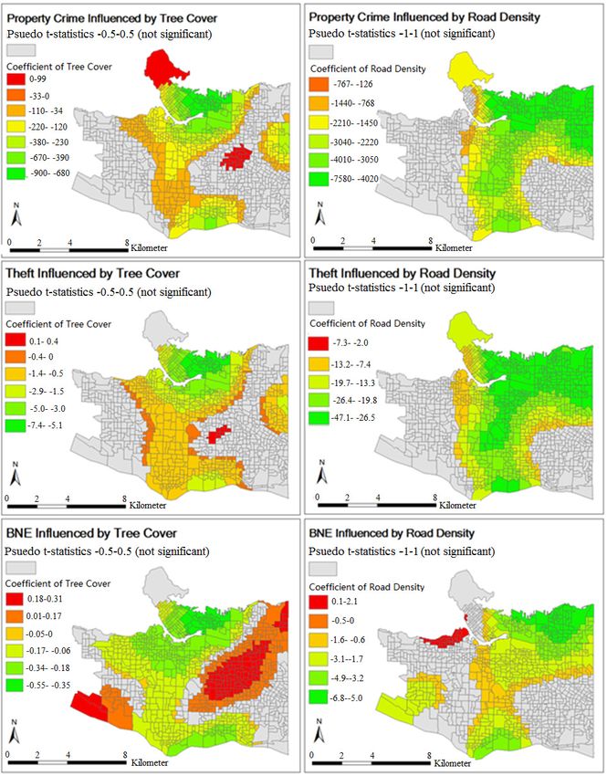
from the GWR tool have their local coefficients for the tested explanatory variables; the variation of the
local coefficients for the percentage of tree covered areas and road density in each model are mapped
(see Figure 2). Pseudo t-statistics were calculated, and the DAs having pseudo t-statistics near zero were
regarded as having non-significant regression results as indicated by the colour grey in the maps.
As shown in the property crime GWR map, the coefficients of percent tree cover become
more negative in the DAs that are closer to the downtown core of Vancouver, thereby expressing
a stronger correlation between property crime rates in the downtown area and the Strathcona
neighborhood. On the other hand, Stanley Park and some residential DAs in the Kensington-Cedar
Cottage neighborhood show a positive, although weaker, correlation between tree coverage and
the property crime rate. The theft GWR maps show similar trends, with relatively smaller actual
values, for the coefficients. The BNE GWR map is different from the maps of property crime and theft.
The negative relationship between percent tree cover and the BNE rate is still greater in downtown
Vancouver and the Southern shoreline, but many more DAs demonstrate positive coefficients that are
significant. Due to the low crime rate of BNE, the magnitude of the coefficients of tree coverage on BNEISPRS Int. J. Geo-Inf. 2018, 7, 101 9 of 14
is much lower than that on theft and total property crime. Road density indicates a greater negative
correlation also in the downtown area and the northeast region to the Hastings-Sunrise neighborhood,
but the
ISPRS variation
Int. is relatively
J. Geo-Inf. 2018, less than
7, x FOR PEER that of the coefficients of the tree coverage.
REVIEW 9 of 14
Figure2.2. Geographically
Figure Geographically Weighted
Weighted Regression
Regression(GWR)
(GWR)maps
mapsshowing
showingspatial
spatialvariation
variationofofthe
thelocal
localtree
coverage coefficients.
tree coverage coefficients.
The regression results provide solid evidence of the inverse relationship between trees and the
property crime rate, and between road density and property crime in Vancouver City. Firstly,
airborne LiDAR data served as a reliable source for deriving tree crown areas and their spatial
distribution in the city, with an overall accuracy of 98.4%. Compared with Landsat imagery, LiDAR
data provides details of tree crowns beside buildings and along city streets. With a set parameter ofISPRS Int. J. Geo-Inf. 2018, 7, 101 10 of 14
The regression results provide solid evidence of the inverse relationship between trees and the
property crime rate, and between road density and property crime in Vancouver City. Firstly, airborne
LiDAR data served as a reliable source for deriving tree crown areas and their spatial distribution in the
city, with an overall accuracy of 98.4%. Compared with Landsat imagery, LiDAR data provides details
of tree crowns beside buildings and along city streets. With a set parameter of 2 m when applying
aggregate points, the extracted tree crown polygons from LiDAR points can be considered to have a
spatial resolution of 2 m × 2 m. In addition to the use of a small unit of analysis, i.e., the dissemination
area, high resolution and accuracy of the extracted tree covered area and calculations led to the precise
estimate of the relationship of the tree covered area with property crime.
Spatial lag regression models prove the qualitative findings with significant negative coefficients
in the regression results. As seen from the spatial lag regression results in Table 2, BNE has a less
negative coefficient in spatial lag, indicating a small magnitude of correlation with trees. Moreover,
the explanatory power of the BNE model, denoted by pseudo R2 , is smaller than that for the other
two models. The first finding could be due to the fact that, compared with theft, BNE has a smaller
incident number. The possible cause of the smaller explanatory power of the BNE model is that the
BNE rate is affected by other factor(s), which may have little influence on other types of property
crime. For example, the BNE rate is more likely related to the distribution of the number and types of
buildings, as well as average family income, security facilities, etc.
Most importantly, GWR, which provides more answers to the research questions, demonstrates
the spatial variation of the correlation between trees and property crime. Significant negative
correlations exist in the central area of the city, and the magnitude of the coefficient becomes greater
in the downtown core of the city. However, unlike other DAs, Stanley Park DA and some of the
Kensington-Cedar Cottage DAs demonstrate a positive correlation between property crime and trees.
According to the geoprocessing results, in 2013 the Kensington-Cedar Cottage neighborhood had
a high tree coverage and a relatively high property crime rate. However, as one of the most ethnically
diverse neighborhoods in east Vancouver, its high crime rate can be a result of a high level of social
disorganization, rather than a high coverage of trees in the neighborhood. Most likely, Stanley Park
had a high property crime rate because it is a tourist attraction, which makes it vulnerable to theft and
mischief. Therefore, the high crime rates are the result of the above factors, rather than merely being the
result of the trees and road network. Also reviewed were the standard residuals of the local regressions
estimated using GWR. The under- and over-estimated results are randomly scattered over the map;
clusters in the map indicate that there are factors that were not taken into account in the model [41].
However, the high regression residuals are concentrated in the northern area of the city, including
Stanley Park and the downtown area. Moreover, as seen from the local R2 values of the GWR results
of the property crime model, local R2 values below 0.2 are clustered in the Renfrew-Collingwood and
Kerrisdale neighborhoods. These are also the results of variations in the social aspect among different
neighborhoods. Important factors, other than the included variables, may be involved.
Counter to the results of the study conducted in the Kitchener-Waterloo region, Ontario, a highly
significant negative correlation was detected between road density and property crime [28]. Because of
the limited number of publications on this topic, we cannot conclude that this disagreement is the result
of variations in the situation of different study areas. In addition, road density is somehow related to
road complexity, with high road density probably suggesting a large number of road segments and a
high level of complexity of the road network. For instance, as denoted by the research conducted in
Tokyo [31], residential areas usually have more roads and greater road densities than commercial areas.
As mentioned, previous research on road networks and crime found that complex road networks
can reduce the number of property crimes. The methodology in our study found only the statistical
relationship between road density and property crime. More study on road characteristics is required
to determine their effects on crime. The findings are the inspiration for planning the urban design
strategies to prevent property crime. The inverse correlation between tree coverage and property
crime suggests it is possible that the Greenest City Action Plan carried out in Vancouver not onlyISPRS Int. J. Geo-Inf. 2018, 7, 101 11 of 14
creates beautiful views and clean air, but also reduces the city property crime rate and provides a safe
living environment for residents. In addition, the downtown core of the city is usually a place with a
high crime rate. According to the GWR maps, because there is a stronger correlation between the tree
coverage and property crime in downtown Vancouver, to reduce the property crime rate, tree planting
projects should be carried out in the downtown core commercial areas. The inverse relationship
between road density and property crime suggests that, to reduce property crime, urban planners
should design complex road networks with more road segments and higher road density within the
urban areas. In regions with lower tree coverage and lower road density, which are regions likely to
have high property crime rates, more police resources should be assigned for crime prevention.
Limitations to this study. First, this study was limited to the city of Vancouver, and some of
the results (e.g., the spatial variation of the influence of trees on crime) are representative only of
areas within the city. A study of the greater Vancouver area could possibly reveal more patterns and
information. Also, similar research should be conducted in other municipalities in Canada to verify
the hypotheses. Besides, this study did not differentiate urban trees along streets and beside buildings
from trees in parks. The extent to which urban property crime can be reduced by planting trees in
these different locations is still uncertain. There must be a detailed analysis of the relation of crime to
urban parks and trees. More importantly, this study performed only a cross-sectional analysis. Further
research is required to determine the causal relationship between the two variables and property crime.
This can be done by performing a temporal crime trend analysis, focusing on areas with significant
changes in vegetation coverage or road density.
Besides, in this study we focused only on property crime and aggregated some of the crime types.
Aggregating different crime types is inappropriate in spatial pattern analysis [43]. For instance, the
spatial patterns of commercial BNE and residential BNE can be very different. Future studies are
required if researchers are to be concerned with spatial patterns for specific crime types, such as thefts
from vehicles, residential BNE, etc. Due to restrictions on the use of violent crime data, this study
did not include an analysis of violent crime data. However, as previously noted, Vancouver also has
a high Crime Severity Index (CSI) that takes into account the seriousness of crime incidents as well,
and violent crime consequences are usually more serious than property crime. Therefore, future work
should investigate the influence of vegetation and road network on violent crime as well. The newly
launched GeoDash web application enables the collection of data regarding incidents of homicides
and crimes against persons.
Furthermore, social and economic developments are changing rapidly and unexpectedly [2].
The use of the 2006 unemployment rate data led to some errors in the regression models. Among
the eight selected independent variables, the unemployment rate, insignificant in all three regression
models, was eliminated in the GWR models. The 2011 census data is the most up to date demographic
data used in this study; however, the actual statistics could have changed in 2013.
In this study, road density was calculated according to the definition provided by the World
Bank. However, this calculation method ignores the other characteristics of a road network such as
width and complexity, which are also correlated to road length. Therefore, the correlation between
road density and property crime is a result of property crime being influenced by other road network
factors. Further studies are needed to take these factors into consideration.
Lastly, the use of the LiDAR dataset in this study was limited to the extraction of classified
tree points. The average height of high vegetation was derived from the dataset and used as
another explanatory variable to investigate if the crime rate is related to tree height. In addition,
such high-spatial resolution LiDAR data, with three-dimensional information, has the potential for the
construction of 3D models for the further development of crime prevention applications.
5. Conclusions
This study contributes to the Canadian literature on Crime Prevention Through Environmental
Design (CPTED) by investigating the relationships between tree coverage and property crime, and roadISPRS Int. J. Geo-Inf. 2018, 7, 101 12 of 14
density and property crime in the city of Vancouver, British Columbia. The key findings of this study are
that, property crime and its two main categories, theft and BNE, have significant inverse relationships
with both the percentage of tree coverage and road density. Moreover, the correlation between trees
and property crime varies spatially, with the greater coefficient concentrated in Downtown Vancouver
and its surrounding neighborhoods. These notable findings provide support for decision making in
urban planning. Planting trees and developing new urban parks can possibly reduce property crime
in Vancouver, especially in the downtown core area. Also, allocating the police force to neighborhoods
with low tree coverage and low road density is an effective way of saving police resources while also
keeping the city safe. Green vegetation provides not only beautiful views, but also clean, fresh air, and
well-developed road networks provide residents with convenience in life. Furthermore, the findings in
this study suggest that a potential benefit of urban trees is a reduction in property crime. In conclusion,
urban planners and city police must cooperate in working toward the simultaneous development of a
sustainable environment and a reduction of crime.
Acknowledgments: This work were supported in part by the National Key Technologies Research and
Development Program of China (2016YFB0502603) and the Key Program of Sichuan science and technology
department. We would like to thank Dongmei Chen at the Department of Geography, Queen’s University, and
Andrea Perrella at the Laurier Institute for the Study of Public Opinion and Policy, Wilfrid Laurier University for
their time and expertise that helped improve this work.
Author Contributions: C.Y. and J.L. conceived and designed the experiments; Y.C. performed the experiments;
C.Y. and Y.C. analyzed the data; J.I., Y.C. and C.Y. wrote and revised the paper.
Conflicts of Interest: The authors declare no conflict of interest.
References
1. Thangavelu, A.; Sathyaraj, S.R.; Balasubramanian, S. Assessment of spatial distribution of rural crime
mapping in India: A GIS perspective. Int. J. Adv. Remote Sens. GIS 2013, 2, 70–85.
2. Ferreira, J.; João, P.; Martins, J. GIS for crime analysis: Geography for predictive models. Electron. J. Inf.
Syst. Eval. 2012, 15, 36–49.
3. Brantingham, P.J.; Brantingham, P.L. (Eds.) Environmental Criminology; Sage Publications: Beverly Hills, CA,
USA, 1981; pp. 27–54.
4. Cozens, P.M.; Saville, G.; Hillier, D. Crime prevention through environmental design (CPTED): A review
and modern bibliography. Prop. Manag. 2005, 23, 328–356. [CrossRef]
5. Weisburd, D.L.; Groff, E.R.; Yang, S.M. The Criminology of Place: Street Segments and Our Understanding of the
Crime Problem; Oxford University Press: Oxford, UK, 2012.
6. Crowe, T.D. Crime Prevention through Environmental Design: Applications of Architectural Design and Space
Management Concepts; Butterworth-Heinemann: Oxford, UK, 2000.
7. Law, J.; Chan, P.W. Bayesian spatial random effect modeling for analyzing burglary risks controlling for
offender, socioeconomic, and unknown risk factors. Appl. Spat. Anal. Policy 2012, 5, 73–96. [CrossRef]
8. Law, J. Health and the environment: A geographical study of drugs at different school neighbourhoods.
In Proceedings of the International Conference on Environmental Science and Development (ICESD 2012),
Hong Kong, China, 5–7 January 2012; pp. 226–232.
9. Fitterer, J.; Nelson, T.A.; Nathoo, F. Predictive crime mapping. Police Pract. Res. 2015, 16, 121–135. [CrossRef]
10. Andresen, M.A. A spatial analysis of crime in Vancouver, British Columbia: A synthesis of social
disorganization and routine activity theory. Can. Geogr. 2006, 50, 487–502. [CrossRef]
11. Troy, A.; Morgan Grove, J.; O’Neil-Dunne, J. The relationship between tree canopy and crime rates across an
urban-rural gradient in the greater Baltimore region. Landsc. Urban Plan. 2012, 106, 262–270. [CrossRef]
12. Wolfe, M.K.; Mennis, J. Does vegetation encourage or suppress urban crime? Evidence from Philadelphia,
PA. Landsc. Urban Plan. 2012, 108, 112–122. [CrossRef]
13. Eckerson, A.W. Understanding the Relationship between Tree Canopy and Crime in Minneapolis, Minnesota Using
Geographically Weighted Regression; Papers in Resource Analysis; Saint Mary’s University of Minnesota Central
Services Press: Winona, MN, USA, 2013; Volume 15, p. 9.ISPRS Int. J. Geo-Inf. 2018, 7, 101 13 of 14
14. Patino, J.E.; Duque, J.C.; Pardo-Pascual, J.E.; Ruiz, L.A. Using remote sensing to assess the relationship
between crime and the urban layout. Appl. Geogr. 2014, 55, 48–60. [CrossRef]
15. Shaw, C.R.; McKay, H.D. Juvenile Delinquency and Urban Areas; University of Chicago Press: Chicago, IL,
USA, 1942.
16. Clear, T.R.; Rose, D.R.; Waring, E.; Scully, K. Coercive mobility and crime: A preliminary examination of
concentrated incarceration and social disorganization. Justice Q. 2003, 20, 33–64. [CrossRef]
17. Wang, F.; Minor, W.W. Where the jobs are: Employment access and crime patterns in Cleveland. Ann. Assoc.
Am. Geogr. 2002, 92, 435–450. [CrossRef]
18. Chen, D.; Weeks, J.V.; Kaiser, J.V., Jr. Remote sensing and spatial statistics as tools in crime analysis. Geogr. Inf.
Syst. Crime Anal. 2004, 270–292. [CrossRef]
19. Riggs, M. Street Lights and Crime: A Seemingly Endless Debate. CityLab. 2014. Available online: http://
www.citylab.com/housing/2014/02/street-lights-and-crime-seemingly-endless-debate/8359/ (accessed on
14 March 2018).
20. Kuo, F.E.; Sullivan, W.C. Environment and Crime in the Inner City. Environ. Behav. 2001, 33, 343–367.
[CrossRef]
21. Garvin, E.C.; Cannuscio, C.C.; Branas, C.C. Greening vacant lots to reduce violent crime: A randomised
controlled trial. Inj. Prev. 2013, 19, 198–203. [CrossRef] [PubMed]
22. Donovan, G.H.; Prestemon, J.P. The effect of trees on crime in Portland, Oregon. Environ. Behav. 2012, 44,
3–30. [CrossRef]
23. Beavon, D.J.; Brantingham, P.L.; Brantingham, P.J. The influence of street networks on the patterning of
property offenses. Crime Prev. Stud. 1994, 2, 115–148.
24. Ye, C.; Cui, P.; Pirasteh, S.; Li, J.; Li, Y. Experimental approach for identifying building surface materials
based on hyperspectral remote sensing imagery. J. Zhejiang Univ. Sci. A 2017, 18, 984–990. [CrossRef]
25. Ye, C.; Wang, M.; Li, J. Derivation of the characteristics of the Surface Urban Heat Island in the Greater
Toronto area using thermal infrared remote sensing. Remote Sens. Lett. 2017, 8, 637–646. [CrossRef]
26. Bogar, S.; Beyer, K.M. Green space, violence, and crime: A systematic review. Trauma Violence Abuse 2015, 17,
160–171. [CrossRef] [PubMed]
27. Gorham, M.R.; Waliczek, T.M.; Snelgrove, A.; Zajicek, J.M. The impact of community gardens on numbers of
property crimes in Urban Houston. HortTechnology 2009, 19, 291–296.
28. Du, Y. How Do Vegetation Density and Transportation Network Density Affect Crime across an Urban
Central-Peripheral Gradient: A Case Study in Kitchener-Waterloo, Ontario. Master’s Thesis, University of
Waterloo, Waterloo, ON, Canada, 2015.
29. Mennis, J. Integrating remote sensing and GIS for environmental justice research. In Urban Remote Sensing:
Monitoring, Synthesis and Modeling in the Urban Environment; Yang, X., Ed.; Wiley-Blackwell: Hoboken, NJ,
USA, 2011; pp. 225–237.
30. Copes, H. Routine activities and motor vehicle theft: A crime specific approach. J. Crime Justice 1999, 22,
125–146. [CrossRef]
31. Murakami, M.; Higuchi, K.; Shibayama, A. Relationship between convenience store robberies and road
environment. In Recent Advances in Design and Decision Support Systems in Architecture and Urban Planning;
Springer: Dordrecht, The Netherlands, 2004; pp. 341–356.
32. Foster, S.; Wood, L.; Christian, H.; Knuiman, M.; Giles-Corti, B. Planning safer suburbs: Do changes in the
built environment influence residents’ perceptions of crime risk? Soc. Sci. Med. 2013, 97, 87–94. [CrossRef]
[PubMed]
33. Statistics Canada. Census Subdivision of Vancouver, CY—British Columbia. 2011 Census Data; 2011.
Available online: https://www12.statcan.gc.ca/census-recensement/2011/as-sa/fogs-spg/Facts-csd-eng.
cfm?LANG=Eng&GK=CSD&GC=5915022 (accessed on 14 March 2018)2011 Census Data.
34. Perreault, S. Police-Reported Crime Statistics in Canada, 2012. Statistics Canada, 2013. Available online:
http://www.statcan.gc.ca/pub/85-002-x/2013001/article/11854-eng.htm (accessed on 14 March 2018).
35. Boyce, J.; Cotter, A.; Perreault, S. Police-Reported Crime Statistics in Canada, 2013. 2014. Available online:
http://www.statcan.gc.ca/pub/85-002-x/2014001/article/14040-eng.htm (accessed on 14 March 2018).
36. Vancouver Police Department (VPD). VPD Launch New GeoDash Crime Map. 2015. Available online: http:
//mediareleases.vpd.ca/2015/12/08/vpd-launch-new-geodash-crime-map/ (accessed on 14 March 2018).ISPRS Int. J. Geo-Inf. 2018, 7, 101 14 of 14
37. Vancouver Police Department (VPD). Data Set Description: Legal Disclaimer from Vancouver Police
Department. 2015. Available online: http://data.vancouver.ca/datacatalogue/crime-data.htm (accessed on
14 March 2018).
38. Anselin, L. Exploring spatial data with GeoDaTM: A workbook. Urbana 2004, 51, 309.
39. Xie, K.; Ozbay, K.; Yang, H. Spatial analysis of highway incident durations in the context of Hurricane Sandy.
Accid. Anal. Prev. 2015, 74, 77–86. [CrossRef] [PubMed]
40. Bidanset, P.E.; Lombard, J.R. Evaluating spatial model accuracy in mass real estate appraisal: A comparison
of geographically weighted regression and the spatial lag model. Cityscape 2014, 16, 169–182.
41. ESRI. Interpreting GWR Results. ArcGIS for Desktop Support. 2016. Available online: http://desktop.
arcgis.com/en/arcmap/latest/tools/spatial-statistics-toolbox/interpreting-gwr-results.htm (accessed on
14 March 2018).
42. Nakaya, T.; Fotheringham, A.S.; Brunsdon, C.; Charlton, M. Geographically weighted Poisson regression for
disease association mapping. Stat. Med. 2005, 24, 2695–2717. [CrossRef] [PubMed]
43. Melo, S.N.; Matias, L.F.; Andresen, M.A. Crime concentrations and similarities in spatial crime patterns in a
Brazilian context. Appl. Geogr. 2015, 62, 314–324. [CrossRef]
© 2018 by the authors. Licensee MDPI, Basel, Switzerland. This article is an open access
article distributed under the terms and conditions of the Creative Commons Attribution
(CC BY) license (http://creativecommons.org/licenses/by/4.0/).You can also read