Unfolding the Earth: Myriahedral Projections
←
→
Page content transcription
If your browser does not render page correctly, please read the page content below
The Cartographic Journal    Vol. 45 No. 1       pp. 32–42      February 2008
# The British Cartographic Society 2008

                                                     REFEREED PAPER

Unfolding the Earth: Myriahedral Projections
Jarke J. van Wijk
Dept. of Mathematics and Computer Science, Technische Universiteit Eindhoven, Eindhoven, The Netherlands
Email: vanwijk@win.tue.nl

   Myriahedral projections are a new class of methods for mapping the earth. The globe is projected on a myriahedron, a
   polyhedron with a very large number of faces. Next, this polyhedron is cut open and unfolded. The resulting maps have a
   large number of interrupts, but are (almost) conformal and conserve areas. A general approach is presented to decide
   where to cut the globe, followed by three different types of solution. These follow from the use of meshes based on the
   standard graticule, the use of recursively subdivided polyhedra and meshes derived from the geography of the earth. A
   number of examples are presented, including maps for tutorial purposes, optimal foldouts of Platonic solids, and a map of
   the coastline of the earth.

INTRODUCTION                                                           are obtained by using different myriahedra and choices for
                                                                       the edges to be cut, which are described in three separate
Mapping the earth is an old and intensively studied
                                                                       sections. The use of graticule-based meshes, recursively
problem. For about two thousand years, the challenge to
                                                                       subdivided polyhedra, and geographically aligned meshes
show the round earth on a flat surface has attracted many
                                                                       lead to different maps, each with their own strengths.
cartographers, mathematicians, and inventors, and hun-
                                                                       Finally, the results are discussed.
dreds of solutions have been developed. There are several
reasons for this high interest. First of all, the geography of
the earth itself is interesting for all its inhabitants. Secondly,
there are no perfect solutions possible such that the surface          BACKGROUND
of the earth is depicted without distortion. Finally, factors          The globe is a useful model for the surface of the earth.
such as the intended use of the map (e.g. navigation,                  Locations on a globe (and the earth) are given by latitude w
visualisation, or presentation), the available technology              and longitude l. The position of a point p(w, l) on a globe
(pen and ruler or computer), and the area or aspect to be              with unit radius is (coslcosw, sinlcosw, sinw). Curves of
depicted lead to different requirements and hence to                   constant w, such as the equator, are parallels; curves of
different optima.                                                      constant l are meridians. A graticule is a set of parallels and
   A layman might wonder why map projection is a problem               meridians at equal spacing in degrees.
at all. A map of a small area, such as a district or city, is             Compared with a map, a globe has some disadvantages,
almost free of distortion. So, to obtain a map of the earth            such as poor portability, and to obtain a more practical
without distortion one just has to stitch together a large             solution, the spherical globe has to be mapped to a flat
number of such small maps. In this article we explore what             surface. This puzzle has intrigued many researchers for two
happens when this naive approach is pursued. We have                   thousand years. John P. Snyder has provided a fascinating
coined the term myriahedral for the resulting class of                 overview of the history of map projection. In the following,
projections. A myriahedron is a polyhedron with a myriad of            references for map projections are only given if not
faces. The Latin word myriad is derived from the Greek                 discussed in his book (Snyder, 1993), to keep the number
word murioi, which means ten thousands or innumerable.                 of references within bounds. Introductions to map pro-
We project the surface of the earth on such a myriahedron,             jection can be found in textbooks on cartography or
we label its edges as folds or cuts, and fold it out to obtain a       geographic visualisation (Robinson et al., 1995; Kraak and
flat map.                                                              Ormeling, 2003; Slocum et al., 2003). Also on the web
   In the next section, some basic notions on map                      much information can be found, for instance in the
projection are presented, and related work is shortly                  extensive website developed by Furuti (2006).
described, followed by a section in which an overview of                  The major problem of map projection is distortion.
the approach employed here is given. Different solutions               Consider a small circle on the globe. After projection on a
DOI: 10.1179/000870408X276594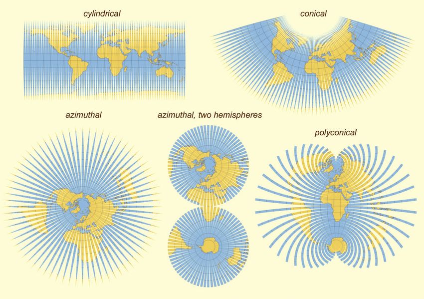
Unfolding the Earth: Myriahedral Projections 33
map, this circle transforms into an ellipse, known as the
Tissot indicatrix, with semi-axes with lengths a and b. If a 5
b for all locations, then angles between lines on the globe
are maintained after projection: The projection is con-
formal. The classic example is the Mercator projection.
Locally, conformality preserves shapes, but for larger areas
distortions occur. For example, in the Mercator projection
shapes near the poles are strongly distorted.
If ab 5 C for all locations on the map, then the
projection has the equal-area property: Areas are preserved
after projection. Examples are the sinusoidal, Lambert’s
cylindrical equal area and the Gall–Peters projection.
The problem is that for a double curved surface no
projection is possible that is both conformal and equal-area.
Along a curve on the surface, such as the equator, both
conditions can be met; however, at increasing distance from
such a curve the distortion accumulates. Therefore,
depending on the purpose of the map, one of these
properties or a compromise between them has to be
chosen. Concerning distortion, uniform distances are
another aspect to be optimised. Unfortunately, no map Figure 1. Distortion in map projection
projections are possible such that distances between any
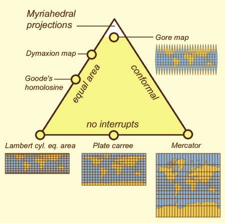
two positions are depicted on a similar scale, but one can cylindrical projections, with linear parallels and meridians.
aim at small variations overall or at proper depiction along Most of the existing solutions, using no interrupts, are
certain lines. located at the bottom of the triangle. In this article, we
Besides these constraints from differential geometry, map explore the top of the triangle, which is still terra incognita,
projection also has to cope with a topological issue. A using geographic terminology. Or, in other words, we
sphere is a surface without a boundary, whereas a finite flat discuss projections that are both (almost) equal area and
area has to be bounded. Hence, a cartographer has to conformal, but do have a very large number of interrupts.
decide where to cut the globe and to which curve this cut Related issues have been studied intensively in the fields
has to be mapped. Many choices are possible. One option, of computer graphics and geometric modelling, for
used for azimuthal projections, is to cut the surface of the applications such as texture mapping, finite-element surface
globe at a single point, and to project this to a circle, meshing, and generation of clothing patterns. The problem
leading to very strong distortions at the boundary. The of earth mapping is a particular case of the general surface
most popular choice is to cut the globular surface along a parameterisation problem. A survey is given by Floater and
meridian, and to project the two edges of this cut to an Hormann (2005). Finding strips on meshes has been
ellipse, a flattened ellipse or a rectangle, where in the last studied in the context of mesh compression and mesh
two cases the point-shaped poles are projected to curves. rendering, for instance by Karni et al. (2002). Bounded-
The use of interrupts reduces distortion. For the distortion flattening of curved surfaces via cuts was studied
production of globes, minimal distortion is vital for by Sorkine et al. (2002). The work presented here has a
production purposes; hence gore maps are used, where different scope and ambition as this related work. The
the world is divided in for instance twelve gores. Goode’s geometry to be handled is just a sphere. The aim is to
homolosine projection (1923) is an equal-area projection, obtain zero distortion, and we accept a large number of
composed from twelve regions to form six interrupted cuts. Finally, we aim at providing an integrated framework,
lobes, with interrupts through the oceans. The projection offering fine control over the results, and explore the effect
of the earth on unfolded polyhedra instead of rectangles or of different choices for the depiction of the surface of the
ellipses is an old idea, going back to Da Vinci and Dürer. All earth.
regular polyhedra have been proposed as suitable candi-
dates. Some examples are Cahill’s Butterfly Map (1909,
octahedron) and the Dymaxion Map of Buckminster Fuller,
METHOD
who used a cuboctahedron (1946) and an icosahedron
(1954). Steve Waterman has developed an appealing We project the globe on a polyhedral mesh, label edges as
polyhedral map, based on sphere packing. cuts or folds, and unfold the mesh. We assume that the
Figure 1 visualises the trade-off to be made when dealing faces of the mesh are small compared with the radius of the
with distortion in map projection. An ideal projection globe, such that area and angular distortion are almost
should be equal-area, conformal, and have no interrupts; negligible. We first discuss the labelling problem. A mesh
however, at most, two of these can be satisfied simulta- can be considered as a (planar) graph G 5 (V, E), consisting
neously. Such projections are shown here at the corners of a of a set of vertices V and undirected edges E that connect
triangle, whereas edges denote solutions where one of the vertices. Consider the dual graph H 5 (V’, E’), where each
requirements is satisfied. Existing solutions can be posi- vertex denotes a face of the mesh, and each edge
tioned in this solution space. Examples are given for some corresponds to an edge of the original graph, but now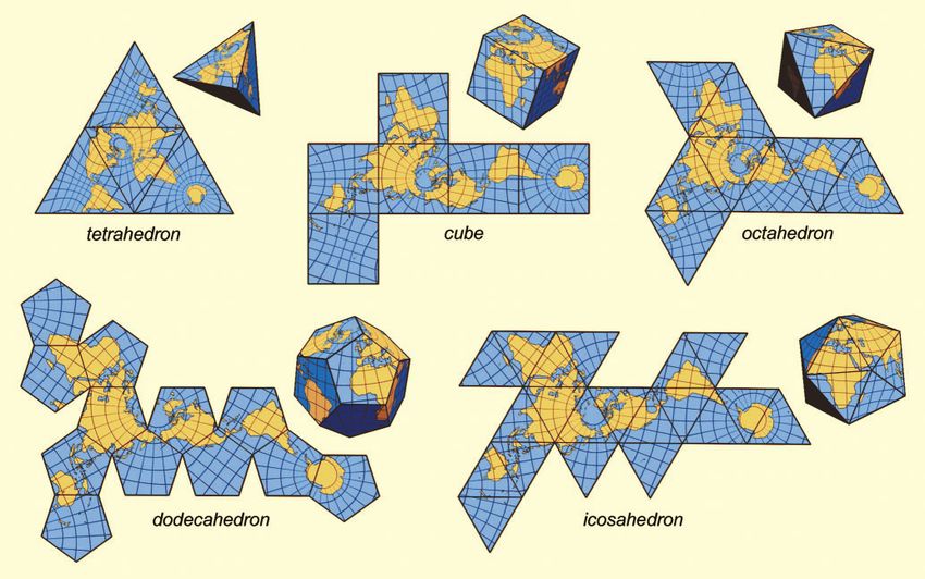
34                                                                                                   The Cartographic Journal

                                                                 the weights its edges is maximal (or minimal). The
                                                                 algorithm to produce a myriahedral projection is now as
                                                                 follows:
                                                                 1.   Generate a mesh;
                                                                 2.   Assign weights to all edges;
                                                                 3.   Calculate a maximal spanning tree Hf;
                                                                 4.   Unfold the mesh;
                                                                 5.   Render the unfolded mesh.
                                                                 In the following sections, we discuss various choices for the
                                                                 first two steps, here we describe the last three steps, which
                                                                 are the same for all results shown.
                                                                    For the calculation of the maximal spanning tree we
                                                                 followed the recommendations given by Moret and
                                                                 Shapiro (1991). We use Prim’s algorithm (Prim, 1957) to
                                                                 find a maximal spanning tree. Starting from a single
                                                                 vertex, iteratively, the neighbouring edge with the
Figure 2. (a) Mesh G; (b) Dual mesh H; (c) Cuts and folds; (d)
Foldout
                                                                 highest weight and the corresponding vertex is added.
                                                                 This gives an optimal solution. The neighbouring edges
                                                                 of the growing tree are stored in a priority queue, for
connecting two faces instead of two vertices (Figure 2).
                                                                 which we use pairing heaps (Fredman, Sedgewick, Sleator
After labelling edges as folds and cuts, we obtain two
                                                                 and Tarjan, 1986). The performance is O(|E | z |V | log
subgraphs Hf and Hc, where all edges of each subgraph are
                                                                 |V |), where |E| and |V | denote the number of edges and
labelled the same. The labelling of edges should be done
                                                                 vertices. In practice, optimal spanning trees are calculated
such that
                                                                 within a second for graphs with ten thousands of edges and
N   the foldout is connected. In other words, in Hf a path       vertices.
                                                                    Unfolding is straightforward. Assume that all faces of the
    should exist from any node (face of the mesh) to any
    other node.                                                  mesh are triangles. Faces with more edges can be handled
N   the foldout can be flattened. Hence, in Hf no cycles         by inserting interior edges with very high weights, such that
                                                                 these faces are never split up. Unfolding is done by first
    should occur, otherwise this condition cannot be met.
                                                                 picking a central face, followed by recursive processing of
Taken together, these constraints imply that Hf should be a      adjacent faces. Consider two neighbouring triangles PQR
spanning tree of H. Also, the subgraph Gc of G with only         and RQS, and assume that the unfolded positions P9, Q9,
edges labelled as cuts should be a spanning tree of G. This      and R9 are known. Next, the angle a between RQS and
can be seen as follows. All vertices should have one or more     the plane of PQR is determined, and S9 is calculated such
cuts in the set of neighbouring edges (otherwise the foldout     that the new angle is a9, |QS | 5 |Q9S9| and |RS | 5 |R9S9|.
can not be flattened), and cycles in the cuts would lead to a    The use of a9 5 0 gives a flat mesh, use of (for instance) a9
split of the foldout. The set of cuts unfolds to a single        5 a(1 z cos(pt/T ))/2 gives a pleasant animation
boundary, with a length of twice the sum of lengths of the       (examples are shown in http://www.win.tue.nl/,
cuts.                                                            vanwijk/myriahedral).
   There is a third constraint to be satisfied: The labelling       The geography of the earth (or whatever image on a
should be such that the foldout does not suffer from fold-       spherical surface has to be displayed) is mapped as a texture
overs. The folded out mesh should not only be planar, it         on the triangles. We use the maps of David Pape for this
should also be single-valued. The use of an arbitrary            (Pape, 2001). When the triangles are large compared with
spanning tree does lead to fold-overs in general. However,       the radius of the globe, like in standard polyhedral
we found empirically that the schemes we use in the              projections, the triangles have to be subdivided further to
following almost never lead to fold-overs, and we do not         control the projection in the interior. We use a simple
explicitly test on this. The problem of fold-overs is complex,   gnomonic projection here.
and we cannot give proofs on this. Nevertheless, it can be          Rendering maps for presentation purposes requires
understood that fold-overs are rare by observing that the        proper anti-aliasing, because regular patterns and very thin
sphere is a very simple, uniform, convex surface; and also,      gaps have to be dealt with. For the images shown, 100-fold
the typical patterns that emerge are strips of triangles,        supersampling per pixel with a jittered grid was used,
connected to and radiating outward from a line or point,         followed by filtering with a Mitchell filter.
which strips rarely overlap.                                        All images were produced with a custom developed,
   The term spanning tree suggests a solution for labelling      integrated tool to define meshes and weights, and to
the edges: Minimal spanning trees of graphs are a well-          calculate and render the results, running under MS
known concept in computer science. Assign a weight w(ei)         Windows. Response times on standard PCs range from
to each of the edges ei, such that a high value indicates a      instantaneous to a few seconds, which enables fast
high strength and that we prefer this edge to be a fold.         exploration of parameter spaces. Rendering of high
Next, calculate a maximal spanning tree Hf (or a minimal         resolution, high quality maps can take somewhat longer,
spanning tree Gc), i.e., a spanning tree such that the sum of    up to a few minutes.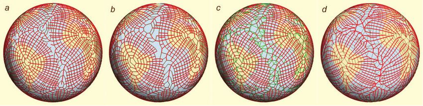
Unfolding the Earth: Myriahedral Projections                                                                                               35

Figure 3. Graticular projections, derived from a 5u graticule. 2592 polygons: a) cylindrical; b) conical; c) azimuthal; d) azimuthal, two hemi-
spheres; e) polyconical

GRATICULES                                                                    The relation between a spatially varying weight w and the
                                                                           decision where to cut and fold can be understood by
The simplest way to define a mesh is to use the graticule
                                                                           considering Prim’s algorithm. Suppose, without loss of
itself, and to cut along parallels or meridians. The results
                                                                           generality, that we start at a maximum of w and proceed to
can be used as an introduction to map projection. A weight
                                                                           attach the edges with the highest weight. At some point,
for edges, using the value of w and l of the midpoint of an                edges at the boundary will have approximately the same
edge, can be defined as                                                    weight and, after a number of additions, a ring of faces is
                                                                           added, with cuts in between neighbouring faces in this ring.
     w(w,l)~{(Ww jw{w0 jzWl min jl{l0 z2pkj),                              Hence, edges aligned with contours of w typically turn into
                                       k
                                                                           folds, whereas edges aligned with gradients of w turn into
where Ww and Wl are overall scaling factors, and w0 and l0                 cuts.
denote where a maximal strength is desired. Different                         Each strip is almost free of angular or area distortion,
values for these lead to a number of familiar looking                      however, a large number of interrupts occur with varying
projections (Figure 3). The use of a high value for Ww                     widths. These gaps visualise, just like the Tissot indicatrix,
gives cuts along meridians. Dependent on the value of                      the distortion that occurs when a non-interrupted map is
w0 a cylindrical projection (0u, equator), an azimuthal                    used, and can be used to explain the basic problem of map
projection (90u, North pole), or a conical projection                      projection. If we want to close these gaps, the strips must
(here 25u) is obtained when the meridian strips are                        be broadened. However, to maintain an equal area, they
unfolded. Use of a negative value for Ww gives two                         have to be shortened, and to maintain the same aspect ratio
hemispheres, each with an azimuthal projection. The                        they have to be lengthened, which is not possible
meridian at which to be centred can be controlled by using                 simultaneously. Also, it is clearly visible that mapping a
a low value for Wl and a suitable value for l0. The use of a               point (such as a pole) to a line leads to a strong distortion.
high value for Wl gives cuts along parallels. Unfolding these                 When the number of strips is increased, the gaps are less
parallels gives a result resembling the polyconic projection               visible, and the distortion is shown via the transparency of
of Hassler (1820).                                                         the map (Figure 4).
36                                                                                                             The Cartographic Journal

                                                                        Figure 6. Close-up of icosahedral projection

                                                                               00          00          00
                                                                             w0 /wc , w1 /w1 ,       wc /(wc zw1 )=2:
Figure 4. Polyconical projection, derived from a 1u graticule,
64 800 polygons                                                         As a result, the weights are highest close to the centre of
                                                                        original edges. Finally, we use wc as the edge weight for the
RECURSIVE SUBDIVISION                                                   edges of the final mesh, plus a graticule weight w with small
For the graticular projections, thin strips of faces are                values for Wl and Ww to select the aspect.
attached to one single strip or face. This is a degenerated                The resulting unfolded maps are, at first sight, somewhat
tree structure. In this section, we consider what results are           surprising (Figure 5). One would expect to see interesting
obtained when a more balanced pattern is used. To this                  fractal shapes, however, at the second level of subdivision
end, we start with Platonic solids for the projection of the            the gaps are already almost invisible (Figure 6). Indeed, the
globe, and recursively subdivide the polygons of these                  structure of the cuts is self-similar, however, for higher
solids. This approach has been used before for encoding                 levels of subdivision and smaller triangles, the surface of the
and handling geospatial data (Dutton, 1996).                            sphere quickly approaches a plane, which has Hausdorff
   At each level i, each edge is split and the new centres,             dimension 2. Only when areas would be removed, such as
halfway on the greater circle connecting the original                   the centre triangles in the Sierpinski triangle, a fractal shape
endpoints, are connected. As a result, for instance each                would be obtained.
triangle is replaced at each level by four smaller triangles.              As a step aside, fractal surfaces and foldouts do not match
Other subdivision schemes can also be used, for instance                well either. Unfolding, for instance, a recursively sub-
triangles can be subdivided into nine smaller ones.                     divided surface with displaced midpoints leads to a large
   The edge weights are set as follows. We associate with               number of fold-overs (Figure 7).
each edge three numbers w0, w1, and wc, where the first two                As another step aside, let us consider optimal mapping on
correspond with the endpoints and the latter with the                   Platonic solids. We consider a map optimal when the cuts
centre position. For new edges, w0 r i, w1 r i, and wc r                do not cross continents. To find such mappings, we assign
iz1. If an edge e is split into two edges e’ and e’’, we use            to each edge a weight proportional to the amount of land
linear interpolation for the new values                                 cut, computed by sampling the edges at a number of
                                                                        positions (here we used 25) and looking up if land or sea is
       0            0           0
     w0 /w0 , w1 /wc ,        wc /(w0 zwc )=2;                          covered in a texture map of the earth. Next, the map is
                                                                        unfolded using the standard method and the sum of
                                                                        weights of cut edges is determined. This procedure is
                                                                        repeated for a large number of orientations of the mesh,
                                                                        searching for a minimal value. We used a sequence of three
                                                                        rotations to vary the orientation of the mesh, and used steps
                                                                        of 1u per rotation. Results are shown in Figure 8.

Figure 5. Recursive subdivision of Platonic solids, using five levels
of subdivision, 4096220 480 polygons                                    Figure 7. Folding out a fractal surface gives a mess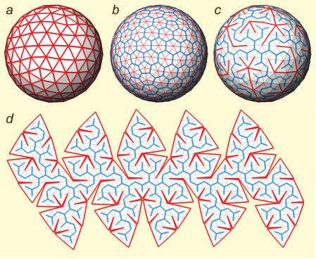
Unfolding the Earth: Myriahedral Projections                                                                                37

Figure 8. Optimal fold-outs of Platonic solids

  For the tetrahedron a perfect, and for the other platonic        where izk is calculated modulo I, L2 5 max(2j,2L), and
solids an almost perfect, mapping is achieved. Except for          Lz 5 min(J212j, L). We typically use I 5 256, J 5 128,
the tetrahedron, the resulting layout of the continents is the     and L 5 32. A large weight mask m is used, because it is not
same as the layout used by Fuller for his Dymaxion map. He         only the edges that have to be blurred, but also areas far
used a slightly modified icosahedron for his best-known            from coastlines must be assigned varying values. The
version, but the version shown here reveals that his               convolution has to be done taking the curvature into
modifications are not necessary per se.                            account; therefore, the width and contents of the mask have
                                                                   to be adapted per scan line. For the width, we use Kjz 5
                                                                   2Kj2 5 qIL/2Jcoswjr. We use a Gaussian filter, taking the
GEOGRAPHY ALIGNED MESHES                                           distance rjkl along a greater circle into account between a
                                                                   centre element R0,j and an element Rk,jzl, as well as the
Taking continents into account when deciding where to cut          area ajl of the latter. Specifically,
is an obvious idea. In this section, we explore this further.
We generate meshes such that continents are cut orthogo-                         Kjz
                                                                                    Lz
                                                                                 X  X
nal to their boundaries. First, we define for each point on             mjkl ~                sjkl ,
the sphere a value f(w, l) that denotes the amount of land in                    k~K {
                                                                                     j l~L{
its neighbourhood. High values are in the centres of
continents, low values in the centres of oceans. This                with
function is used to generate the mesh, and also to control                                           pffiffiffiffiffiffi
                                                                                          2
the strength of edges. We use linear interpolation of a                 sjkl ~ajkl exp ({rjkl =2s2 )= 2ps,
matrix of values Fij, with i 5 0,..., I21 and j 5 0, ..., J21 to
calculate f(w, l). The corresponding values for l and w per             ajl ~2p2 cos wjzl =NM , and
element are li 5 2p(iz0.5)/I and wj 5 p(jz0.5)/J 2 p/                                h                     i
2, respectively. The matrix F is derived from a raster image            rjkl ~ arccos p(wj ,0):p(wjzl ,lk ) :
R of a map with the same dimensions as F via convolution
with a filter m, i.e.,                                             Figure 9 shows an example. As a result, for instance the
                                                                   value for the South Pole is similar to that of the centre of
             Kj
             X
               z
                Lz
                X                                                  South America.
     Fij ~                mjkl Rizk,jzl ,                             To obtain a foldout with cuts perpendicular to contours
             k~K {
                 j l~L{                                            of f, the following steps are performed (Figure 10), inspired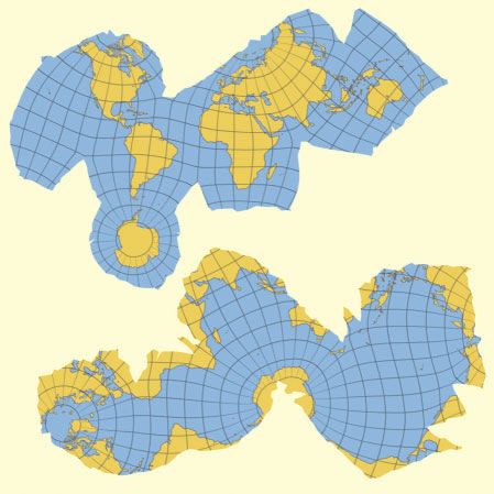
38                                                                                                              The Cartographic Journal

                                                                            is traced; lines perpendicular to contours follow from
                                                                            tracing the vector field
                                                                                                           .qffiffiffiffiffiffiffiffiffiffiffiffiffiffiffiffiffiffiffiffiffiffiffiffiffiffiffi
                                                                               g(w,l)~(fw cos w,fl = cos w)  cos2 wfw2 zfl2 , where

                                                                               fl ~Lf (w,l)=Ll and fw ~Lf (w,l)=Lw:

                                                                         The factors cosw in the definition of c and g follow from the
                                                                         requirements that we want these fields to have a unit
                                                                         magnitude and to be orthogonal after projection on the
                                                                         sphere. Projection implies that components Dl of a vector
                                                                         (Dw, Dl) are scaled with a factor cosw, whereas the Dw
                                                                         components keep their length. For the tracing, we use a
                                                                         fourth order Runge–Kutta method with a fixed time step.
                                                                            In the next step, crossings between these line sets are
                                                                         calculated and the lines are cleaned up. Streamlines without
Figure 9. From R to F via convolution with a Gaussian
                                                                         crossings are removed, neighbouring points of crossings are
by the anisotropic polygonal remeshing method of Alliez                  removed from the streamlines, and heads and tails are
et al. (2003):                                                           removed. Next, the resulting net is scanned and a set of
                                                                         polygons, covering the sphere, is constructed. This gives a
a. Generate mesh lines along and perpendicular to                        regular, rectangular mesh for a large part of the sphere, but
   contours of f with the algorithm of Jobard and Lefer                  also and unfortunately, irregular polygons. This can be
   (Jobard and Lefer, 1997);                                             understood from the topology of vector fields, a well-
b. Calculate intersections of these sets of lines, and derive            known topic in the visualisation community (Helman and
   polygons;                                                             Hesselink, 1991). Critical points are points where the
c. Tesselate polygons with more than four edges; and                     magnitude of the vector field is zero. For the vector fields
   finally                                                               used here, these occur at maxima of f (centres of
d. Use the standard approach to decide on folds and cuts.                continents), minima of f (centres of oceans) and at
                                                                         saddle-points of f (for instance between South America
These steps are discussed in more detail.
                                                                         and Africa). The domain of a flow field can be tessellated
   The algorithm of Jobard and Lefer (Jobard and Lefer,
                                                                         using streamlines between these critical points, the so-called
1997) is an elegant and fast method to produce equally
                                                                         separatrices, which gives a topological decomposition of the
spaced streamlines for a given vector field. Starting from a
                                                                         domain. For the vector fields used here, separatrices
single streamline, new streamlines are repeatedly started                typically run through valleys of f. When f is used to decide
from seedpoints at a distance d from points of existing                  which edges to label as cuts, the surface breaks along those
streamlines, and traced in both directions. If such a                    valleys, which in turn appear as overall boundaries.
streamline is too close to an existing streamline or when a              Downhill gradient lines of f, following g, bend into such
cycle is formed, the tracing is stopped. The time critical step          valleys with a sharp turn or stop because a line at the other
is to determine which points are close. The standard                     side is too close, leading to irregular polygons.
solution is to use a rectangular grid for fast look-up. Here                We use a standard triangulation algorithm to tessellate
streamlines are traced in (w, l) space, and the mapping to               polygons with more than four edges. First, the polygon is
the sphere has to be taken into account. We therefore use                split into convex polygons, next, triangles are split off.
horizontal strips of rectangles, where the number of                     Heuristics used are a preference for short inserted edges and
rectangles per strip is proportional to cosw.                            avoidance of obtuse or very sharp angles. This is not perfect
   To obtain mesh lines along contours, the vector field                 yet and leads to a somewhat fractured and irregular
                       .qffiffiffiffiffiffiffiffiffiffiffiffiffiffiffiffiffiffiffiffiffiffiffiffiffiffiffi                     appearance of the map when unfolded. Improvement turns
     c(w,l)~(fl ,{fw )     cos2 wfw2 zfl2                                out not to be simple. In an image like Figure 10(c) it is easy

Figure 10. Use of contours and gradients to derive a mesh: a) Jobard and Lefer algorithm; b) finding polygons; c) triangulation; d) deciding
on cuts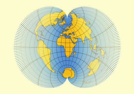
Unfolding the Earth: Myriahedral Projections                                                                                 39

Figure 11. Same as Figure 10, using curvature tensor field

to point at polygons where better choices could have been         DISCUSSION
made, the hard part is to find methods that have no adverse
                                                                  We have presented a new class of map projections, based on
effect at other locations. For instance, introducing extra        projecting the earth on myriahedra, polyhedra with many
points and edges often leads to more irregularities, and          faces, and unfolding these. A general approach is presented
tracing lines between critical points in advance gives wide       to decide on cuts and folds, based on weighting the edges
interrupts instead of multiple smaller ones.                      and calculating a maximal spanning tree. Three different
   We also tried the use of a tensor field based on curvature     choices for types of meshes and weighting schemes are
(Alliez et al., 2003), instead of a vector field (Figure 11).     presented, leading to a variety of different projections of the
Here, at each point, the direction of minimum or maximum          surface of the earth.
curvature is traced. This gives an orthogonal mesh, without          There remains one question to be answered: What is this
singularities along lines and, indeed, the valley in the centre   all good for? Most resulting maps are highly unusual, and
of the Atlantic Ocean is now filled in a more regular way.        do not correspond with what on average is considered to be
However, this does not necessarily lead to a more appealing       a useful map.
tessellation, see for instance the small strip introduced in         Furthermore, the complexity is high. Standard projection
the centre of this valley. Tensor fields have two kinds of        methods require, in the worst case, a few iterations per
singular points: trisectors and wedges. Here, a trisector         point to solve a transcendental equation; the methods
appears in the northern Atlantic Ocean, and a wedge in the        presented here require implementation of a number of non-
Gulf of Guinea. This latter feature leads to irregularities in    trivial algorithms. Hence, forward mapping is not easy, and
the resulting mesh.                                               also inverse mapping, from a location on the map to a point
   Other solutions are to increase the density of the mesh,       on the globe, is much more involved than with standard
and, simply to accept the fractured boundaries. Visually,         maps.
they show that the surface of the globe is torn apart, and           Fortunately, there are also positive aspects that can be
they show that where this is done exactly is somewhat             mentioned. From an academic point of view, a classic topic
arbitrary.                                                        like map projection deserves an exhaustive exploration and
   Figure 12 shows results of this approach. Straightforward      this class of maps has not been addressed yet. What happens
application leads again to the layout of the continents of        when many small maps are glued together is obvious and
Buckminster Fuller. A more familiar layout can be obtained        here an extensive answer is given. Hence, these maps could
by adding a graticular weight, and tuning Wl and Ww. The          be used for textbook purposes. Furthermore, each class has
overall layout resembles a conical projection. The con-           its own interesting aspects. The graticular maps can be used
tinents are shown with few interrupts and with correct            to explain the basics of map projection. Polyhedral maps are
shape and relative position. Instead of f, also |f 2 fc| can be   entertaining, and here we have presented optimal versions.
used as a weight for the edges. As a result, the global              We have investigated what happens when interrupts are
boundary of the map is along contours f 5 fc. This                removed. In Figure 13, two examples are shown, derived
boundary is smooth, and divides the surface here into the         from maps shown in Figure 12. We matched corresponding
main continents, the oceans, and Antarctica. The author           vertices at a distance below a certain threshold, starting at
does not know a similar map.                                      the ends of gaps, followed by a finite element simulation to
   Also, 2f can be used as a weight for the edges. This           redistribute the points of the mesh. In the examples shown,
results in a map where the oceans are central, surrounded         we defined the stiffness matrix such that the equal-area
by the coastline of the world. Ocean centred maps have            property is satisfied. These steps are repeated until no
been made before, such versions are available for Goode’s         corresponding vertices could be found. The maps are not
homolosine map and Fuller’s Dymaxion map. Closest is a            conformal: Parallels and meridians do not cross at right
map presented by Athelstan Spilhaus (Spilhaus, 1983). His         angles. The hard boundaries of the maps without interrupts
map (and also Fuller’s) is centred on Antarctica, showing         are somewhat arbitrary, but do attract attention, in contrast
the oceans as three lobes, and is, hence, somewhat less           to the more fuzzy boundaries of their myriahedral counter-
extreme than the version shown here. A map similar to             parts. Finally, they reveal a quality of all myriahedral maps.
Spilhaus’s map can easily be generated with our method,           The interrupts present in myriahedral maps show the
simply by removing Antarctica from the map R.                     inevitable distortion in a natural, and explicit way, whereas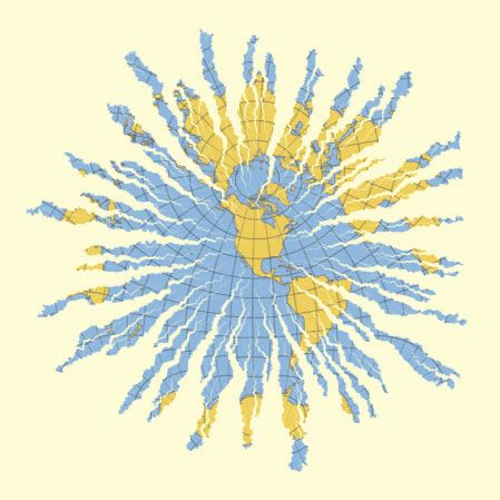
40                                                                                                      The Cartographic Journal

Figure 12. Myriahedral projections with geography aligned meshes, 5500 polygons

in standard maps it is left to the viewer to guess where and          not simple, but when the machinery is set up, a very large
which distortion occurs.                                              variety of maps can be generated just by changing
   Methodologically interesting is that here a computer               parameters, such as Wl, Ww, F, f0, s, and the size of the
science approach is used, whereas map projection is                   faces used. This leaves much room for serendipity, and
traditionally the domain of mathematicians, cartographers,            indeed, some of the maps shown here were discovered by
and mathematical cartographers. Myriahedral projections               accident.
are generated using algorithms, partially originating from               Maps are not only used for navigation or visualisation,
flow visualisation, and not by formulas. Implementation is            but also for decorative, illustrative and even rhetoric
Unfolding the Earth: Myriahedral Projections                                                                                    41

Figure 13. Closed gaps                                           Figure 14. Azimuthal projection, random weights added, 81 920
                                                                 polygons

purposes (Monmonier, 1991), for instance on covers of            angles. Such applications can be produced easily, just by
magazines. The coastline map is an example, which can            varying the map used for mesh alignment.
serve to emphasise the importance of oceans. Another
example is shown in Figure 14. Here, we used a subdivided
icosahedral projection, centred at 40uN, 100uW, and used
                                                                 BIOGRAPHICAL NOTE
an edge weight proportional to the distance from this
point, plus a small random factor.                                                              Jarke J. van Wijk is a full
   As a first step to a user study, the resulting projections                                   professor of Visualisation at
were shown as static images and in animated version to                                          the Technische Universiteit
about 20 people, ranging from laymen via computer                                               Eindhoven. He has a MSc
scientists to cartographers. In general, the reception was                                      in Industrial Design and a
very positive. Most people found the results compelling and                                     PhD in Computer Science,
intriguing. Computer science colleagues liked the general                                       both from the Delft
framework and the algorithms. Nevertheless, taking a                                            University of Technology.
utilitarian point of view, some cartographers argued that                                       His main research interests
cuts are always more disturbing reading a map than having                                       are             Information
distortion, which is the reason that such projections have                                      Visualisation and Flow
been discarded so far and are not useful in practice.                                           Visualisation, with a focus
Concerning usability for tutorial purposes, results were                                        on developing novel and
mixed again. Some cartographers found this a very strong                                        effective visual representa-
feature; others argued that visualising a distorted grid                                        tions. He has been paper
would be more effective. More elaborate usability tests are      co-chair of the IEEE Visualisation and IEEE Information
required to evaluate which approach is most effective here       Visualisation conferences.
and, also, to see what the value is in general. Besides such a
lab test, an interesting test is whether these results are
interesting for, and find their way to, a large audience. So     ACKNOWLEDGEMENTS
far the results were only shown under non-disclosure
conditions, so we cannot report on that yet. It is               The author thanks Michiel Wijers for coining the term
encouraging, however, that many viewers asked when the           ‘myriahedral’, and Jason Dykes and Menno-Jan Kraak for
results would become publicly available and if they could be     their encouragement and advice.
notified on this.
   There is room for more future work. We are considering
                                                                 REFERENCES
alternative methods to produce geography aligned meshes.
An interesting option is to use a physically based model to      Alliez, P., Cohen-Steiner, D., Devillers, O., Levy, B. and
simulate crack formation (Iben and O’Brien, 2006). Also,             Desbrun, M. (2003). ‘Anisotropic polygonal remeshing’, ACM
                                                                     Transactions on Graphics 22(3), 485–493. Proceedings
the methods presented here can be used for a variety of              SIGGRAPH 2003.
other purposes, for instance to show plate tectonics,            Dutton, G. (1996). ‘Encoding and handling geospatial data with
voyages of discovery, or scientific data given for spherical         hierarchical triangular meshes’, in Advances in GIS Research II
42 The Cartographic Journal (Proc. SDH7, Delft, Holland), 505–518, ed. by Kraak, M.-J. and Moorhead, R., Gross, M. and Joy, K.I., IEEE Computer Society Molenaar, M., Taylor & Francis, London. Press. Floater, M. S. and Hormann, K. (2005). ‘Surface parameterisation: a Kraak, M.-J. and Ormeling, F. (2002). Cartography: Visualization of tutorial and survey’, in Advances in multiresolution for geo- Geospatial Data (2nd edition), Prentice Hall, London. metric modelling, 157–186, ed. by Dodgson, N. A., Floater, M. S. Monmonier, M. (1991). How to Lie with Maps, University of and Sabin, M. A. (eds), Springer Verlag. Chicago Press, Chicago. Fredman, M. L., Sedgewick, R., Sleator, D. D. and Tarjan, R. (1986). Moret, B. M. E. and Shapiro, H. D. (1991). ‘An empirical analysis of ‘The pairing heap: A new form of self-adjusting heap’, algorithms for constructing a minimum spanning tree’, Lecture Algorithmica 1(1), 111–129. Notes in Computer Science 555, 192–203, Springer Verlag. Furuti, C. A. (2006). ‘Map Projections’ http://www.progonos.com/ Pape, D. (2001). ‘Earth images’, www.evl.uic.edu/pape/data/Earth. furuti/MapProj. Prim, R. (1957). ‘Shortest connection networks and some general- Helman, J. L. and Hesselink, L. (1991). ‘Visualizing vector field isations’, Bell System Technical Journal 36, 1389–1401. topology in fluid flows’, IEEE Computer Graphics and Robinson, A. H., Morrison, J. L., Muehrcke, P. C. and Kimerling, A. J. Applications 11(3), 36–46. (1995). Elements of Cartography, Wiley. Iben, H. N. and O’Brien, J. F. (2006). ‘Generating surface crack Slocum, T. A., McMaster, R. B., Kessler, F. C. and Howard, H. H. patterns’, in Proceedings of the 2006 ACM SIGGRAPH/ (2003). Thematic Cartography and Geographic Visualization, Eurographics Symposium on Computer Animation, SCA Second Edition, Prentice Hall. 2006, Vienna, Austria, 177–185, ed. by O’Sullivan, C. and Snyder, J. P. (1993). Flattening the Earth: Two Thousand Years of Pighin, F., Eurographics association, Aire-la-Ville, Switzerland. Map Projections, University of Chicago Press. Jobard, B. and Lefer, W. (1997). ‘Creating evenly-spaced stream- Sorkine, O., Cohen-Or, D., Goldenthal, R. and Lischinski, D. (2002). lines of arbitrary density’, in Visualization in Scientific ‘Bounded-distortion piecewise mesh parameterisation’, Proceed- Computing ’97, 43–56, ed. by Lefer, W. and Grave, M., ings of IEEE Visualization 2002, 355–362, ed. by Moorhead, Springer Verlag. R., Gross, M. and Joy, K.I., IEEE Computer Society Press. Karni, Z., Bogomjakov, A. and Gotsman, C. (2002). ‘Efficient Spilhaus, A. (1983). ‘World ocean maps: The proper places to compression and rendering of multi-resolution meshes’, interrupt’, Proceedings of the American Philosophical Society Proceedings of IEEE Visualization 2002, 347–354, ed. by 127(1), 50–60.
You can also read