Resonant subwavelength control of the phase of spin waves reflected from a Gires-Tournois interferometer
←
→
Page content transcription
If your browser does not render page correctly, please read the page content below
www.nature.com/scientificreports
OPEN Resonant subwavelength control
of the phase of spin waves
reflected from a Gires–Tournois
interferometer
Krzysztof Sobucki1*, Wojciech Śmigaj2, Justyna Rychły3, Maciej Krawczyk1 &
Paweł Gruszecki1*
Subwavelength resonant elements are essential building blocks of metamaterials and metasurfaces,
which have revolutionized photonics. Despite similarities between different wave phenomena,
other types of interactions can make subwavelength coupling significantly distinct; its investigation
in their context is therefore of interest both from the physics and applications perspective. In this
work, we demonstrate a fully magnonic Gires–Tournois interferometer based on a subwavelength
resonator made of a narrow ferromagnetic stripe lying above the edge of a ferromagnetic film. The
bilayer formed by the stripe and the film underneath supports two propagative spin-wave modes, one
strongly coupled with spin waves propagating in the rest of the film and another almost completely
reflected at the ends of the bilayer. When the Fabry–Perot resonance conditions for this mode are
satisfied, the weak coupling between both modes is sufficient to achieve high sensitivity of the phase
of waves reflected from the resonator to the stripe width and, more interestingly, also to the stripe-
film separation. Such spin-wave phase manipulation capabilities are a prerequisite for the design
of spin-wave metasurfaces and may stimulate development of magnonic logic devices and sensors
detecting magnetic nanoparticles.
The recent years have been marked by a rapidly growing demand for interconnected mobile devices. This emerg-
ing ecosystem of connected devices, preferably communicating wirelessly, is referred to as the Internet of Things.
There are estimations that within the next few years, the number of WiFi-enabled devices will be at least four
times larger than the total population of the world1. One of the essential components of the Internet of Things
are small and energetically efficient devices processing signals converted from and then back to microwaves,
within the edge computing paradigm. In this field, the application of spin waves (SWs), which are collective
disturbances of magnetization oscillating at the same frequency range as microwaves and thus able to couple to
them, opens up a new opportunity to increase the efficiency and functionality of microwave devices. Compared
to exsisting microwave devices, SW components offer prospects for increased miniaturization (SWs can have
wavelengths 3–5 orders of magnitude shorter than microwaves of the same frequency), easy external control of
SW signals, reprogrammability, and significant decrease of energy demands due to lack of Joule heating related
to SWs p ropagation2–4. In order to use this kind of waves as an information carrier, efficient methods of their
excitation and control over their amplitude and phase must be developed.
In modern photonics, a breakthrough in the control of reflected and transmitted waves at subwavelength
distances has recently been achieved through the use of arrays of nanostructured antennas absorbing and ree-
mitting modified electromagnetic w aves5,6. These arrays, so-called metasurfaces, are used to obtain anomalous
refraction of incident waves or to design flat, ultra-narrow lenses able also to form holograms. Moreover, such
nanostructured antennas can serve as color filters with subwavelenght pixels for printing purposes, as a replace-
ment of chemical dyes7,8.
There are several reports on the SW coupling of an uniform ferromagnetic film with small magnetic ele-
ments. Kruglyak et al. have shown that a narrow ferromagnetic element placed on top of a magnetic waveguide
can be used to emit SWs, to control the phase of SWs passing below the resonator, and under some conditions
even to absorb the energy of propagating SWs9–11. Yu at al. have demonstrated chiral excitation of SWs in a thin
1
Faculty of Physics, Adam Mickiewicz University, Uniwersytetu Poznanskiego 2, 61‑614 Poznan, Poland. 2Met
Office, FitzRoy Rd, Exeter EX1 3PB, UK. 3Institute of Molecular Physics, Polish Academy of Sciences, Mariana
Smoluchowskiego 17, 60‑179 Poznan, Poland. *email: krzsob@amu.edu.pl; gruszecki@amu.edu.pl
Scientific Reports | (2021) 11:4428 | https://doi.org/10.1038/s41598-021-83307-9 1
Vol.:(0123456789)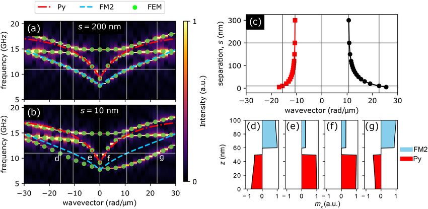
www.nature.com/scientificreports/
Figure 1. Geometry of the system used in simulations. A ferromagnetic stripe of width w and thickness d2 is
separated from a semi-infinite permalloy film of thickness d1 by a distance s. The right edges of both layers are
aligned at x = w . The whole system is placed in an external magnetic field µ0 H0 = 0.1 T parallel to the y axis.
The geometry of the system is independent from y.
film through its dipolar coupling with a single nanowire or a grating of nanowires placed in a spatially uniform
microwave-frequency magnetic fi eld12,13. Subsequently, the existence of Fano resonances and their influence
on the amplitude and phase of transmitted waves in a single-mode waveguide has been studied further by Al
et al.14, and Zhang et al. have demonstrated the application of a single dynamically tunable resonator in zero bias
field placed on top of a waveguide to tune the phase of the transmitted S Ws15. A grating coupler made up of an
array of resonators has been used to excite short-wavelength S Ws16,17, and Graczyk et al.18 have demonstrated
that dynamical coupling of a homogeneous ferromagnetic film with a periodic array of ferromagnetic stripes
placed underneath can lead to the formation of a magnonic band structure in the film. However, the effect of a
resonator on the phase of the reflected wave has not yet been studied in magnonics; moreover, the conditions
for the existence of Fabry–Perot resonances and their effect on both reflected and transmitted SWs, especially
at subwavelength distances, remain almost u nexplored19, while both may be key ingredients in creating a mag-
nonic metasurface.
In this paper, we investigate theoretically the interaction of a narrow, subwavelength-width stripe placed
above the edge of a homogeneously magnetized film with propagating SWs, study its influence on the phase
shift of reflected SWs, and finally demonstrate a magnonic Gires–Tournois interferometer20. Using frequency-
domain finite-element (FD-FEM) calculations and micromagnetic simulations we find that this shift depends
on the width of the stripe in a non-trivial way: an overall slow and steady increase of the phase shift with stripe
width is repeatedly interrupted by sharp phase jumps by 360◦ . Treating the stripe and the underlying film as a
non-reciprocal waveguide supporting two pairs of counter-propagating modes, we formulate a semi-analytical
model that explains this behavior as a consequence of Fabry–Perot resonances produced by one of these mode
pairs. We also show that by varying the film-stripe separation it is possible to switch between resonances of
different order. Our results point to the importance of Fabry–Perot resonances appearing in locally bilayered
ferromagnetic elements, with potential applications for the control of SW propagation in magnonic devices at
subwavelength distances.
Results and discussion
Structure under consideration. We consider a system composed of non-magnetic and ferromagnetic
materials. Its geometry is independent of the y coordinate and piecewise constant along x, as shown schemati-
cally in Fig. 1. The system consists of a semi-infinite permalloy (Py) film of thickness 50 nm and a ferromag-
netic stripe of thickness 40 nm and finite width w. Both elements are separated by a distance s and their right
edges are aligned to x = w . Throughout the paper, we will vary the width w of the stripe and its separation s
from the film. We are interested in manipulating the phase of the reflected SWs using subwavelength elements;
therefore the width of the stripe will be smaller than or comparable to the wavelength of SWs in the Py film at
the frequency of operation. The system is magnetized by a uniform in-plane bias magnetic field of magnitude
µ0 H0 = 0.1 T directed along the y axis. In all calculations we have taken the saturation magnetization of the film
to be MS = 760 kA/m and its exchange constant, Aex = 13 pJ/m. The stripe is made of a material (called FM2
from here on) with MS = 525 kA/m and Aex = 30 pJ/m; lowering its saturation magnetization and increasing
the exchange constant with respect to Py will allow us to exploit interactions of local resonances of the stripe with
propagating waves in Py at frequencies characteristic for the dipolar and dipole-exchange SWs. Such a choice of
the stripe’s material shifts the SW spectrum down and flattens the first band for lower wavevectors with respect
to the Py, as will be discussed in the next section. The gyromagnetic ratio of both ferromagnets is γ = −176 rad
GHz/T.
Scientific Reports | (2021) 11:4428 | https://doi.org/10.1038/s41598-021-83307-9 2
Vol:.(1234567890)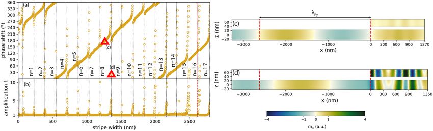
www.nature.com/scientificreports/
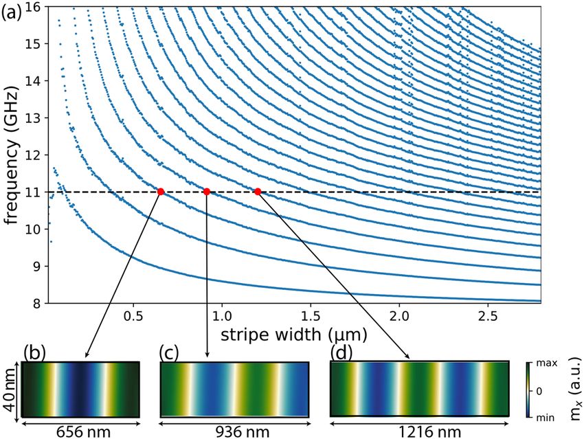
Figure 2. (a,b) Dispersion relations calculated for two infinite films made of Py and FM2 separated by a non-
magnetic spacer of width (a) 200 nm and (b) 10 nm. Colormaps in the background present results obtained by
means of micromagnetic simulations, whereas green points correspond to the results of FD-FEM calculations.
The dashed blue and the dash-dotted red lines are the analytical dispersion relations of SWs supported by
isolated FM2 and Py films, respectively. The horizontal line marks the frequency f = 11 GHz used in further
calculations. (c) Dependence of the wavenumber of the slow modes, marked with d and g in (b), located
predominantly in FM2, on the separation between films at frequency 11 GHz. (d–g) Profiles of the dynamic mx
component of the magnetization (normalized to a maximum of 1) of the (d), (g) slow and (e,f) fast modes of the
Py/FM2 bilayer with spacer width 10 nm at frequency 11 GHz. The positions of these modes on the dispersion
diagram are marked with letters d–g in panel (b).
Dispersion relation of bilayers. Before we study the coupling of a film with a finite-width stripe and SW
reflection, let us first analyze the interaction between modes in infinitely extended films, i.e., in bilayers com-
posed of an infinite Py film separated by a non-magnetic spacer from another infinite film made of FM2. Two
example dispersion relations calculated using micromagnetic simulations and FD-FEM (see the “Methods” sec-
tion for details) for bilayers with separations s = 200 nm and s = 10 nm are presented in Fig. 2a,b, respectively.
It is clear that for a 200 nm-wide separation, the SW modes in Py and FM2 almost do not interact with each
other: the calculated dispersion curve coincides with the analytical dispersion curves of isolated Py and FM2
films calculated using [21, Appendix C.7]:
2
ωM
ω2 = ω0 (ω0 + ωM ) + 1 + e−2kd , (1)
4
where d is the film thickness, ω = 2πf is the angular frequency of SWs (f denotes the frequency), k is the wave-
number, ω0 = |γ |µ0 (H0 + MS l 2 k2 ) [ 22, Chapter 7.1], l = 2Aex /(µ0 MS2 ) is the exchange length, and
ωM = |γ |µ0 MS.
The only visible difference occurs at frequencies above 14 GHz where we can see a hybridization between the
fundamental SW mode and the first mode quantized across the thickness, a so-called perpendicular standing
SW21. This hybridization and perpendicular standing SWs, however, are not considered in the analytical model
and in investigations presented in the following part of the paper.
At frequencies below 14 GHz the modes in the bilayered structure can be classified according to their ori-
gin and group velocity. The fast modes are related to SW dynamics in Py (see Fig. 2e,f) and are characterized
by steeper dispersion (therefore higher group velocity) and longer wavelengths. In contrast, the slow modes
originating in FM2 (see Fig. 2d,g) have lower group velocity and shorter wavelengths. It is worth noting that
the wavelengths of SWs in separated layers do not depend on the direction of propagation, while the dynamic
dipolar coupling between SW modes in both layers combined with the nonreciprocal nature of surface SW modes
introduces asymmetry23–25. For s = 200 nm the coupling is still very weak and at the frequency of 11 GHz, which
is used in further analysis and marked with the white horizontal line in Fig. 2a, the fast and slow modes have
wavelengths of 2660 nm and 590 nm, respectively, for both propagation directions.
Reduction of the non-magnetic spacer width to s = 10 nm causes strong interaction between the modes.
The wavelength of the slow modes decreases significantly and their dispersion relation becomes strongly non-
reciprocal; at 11 GHz, the slow mode propagating leftwards has wavelength 390 nm and the one propagating
rightwards, 270 nm. Fig. 2c shows that the asymmetry of the dispersion relation for slow modes grows as the
films are brought closer to each other.
Scientific Reports | (2021) 11:4428 | https://doi.org/10.1038/s41598-021-83307-9 3
Vol.:(0123456789)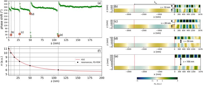
www.nature.com/scientificreports/
Figure 3. (a) Dependence of the frequency of stripe modes on the stripe width. The dashed line marks the
frequency f = 11 GHz. (b–d) Profiles of modes supported by stripes of width 656 nm, 936 nm, and 1216 nm at
frequency 11 GHz.
Eigenmodes of finite‑width stripes. The dependence of the eigenmode spectrum of an isolated finite-
width FM2 stripe on its width is displayed in Fig. 3a. These calculations were made with FD-FEM for the first
thirty modes of stripes with widths up to 2800 nm; note that SW wavelength in uniform Py films at 11 GHz is
2660 nm. As intuitively expected, mode frequency decreases with increasing stripe width. The horizontal dashed
line in Fig. 3 marks f = 11 GHz. It is visible that stripes of multiple widths support modes at this frequency.
Profiles of three successive modes (for stripes of width 656 nm, 936 nm, and 1200 nm) are shown in Fig. 3b–d.
Successive resonances appear for stripes of widths differing by approximately half of the wavelength of the eigen-
mode of a homogeneous FM2 film, i.e., w ≈ 280 nm ≈ 0.5 FM2.
Lateral mode confinement in a reciprocal medium leads to formation of standing waves and quantization
of the wavenumber. The standing waves have the form exp(ikn x) + exp(−ikn x), where n is the mode index,
kn = rn π/w and rn = n + δ ( 0 ≤ δ ≤ 1). For the Dirichlet (magnetic wall) boundary conditions, with the
dynamic magnetization vanishing at the edges, we get rn = n + 1, whereas for “free spins” at the edges, rn = n.
However, due to dipolar interactions, in magnetic stripes neither of these boundary conditions is correct and
the magnetization is partially pinned at the stripe edges, 0 < δ < 126,27. This can also be interpreted as the
effective width of the waveguide being slightly larger than the real one, or in terms of a non-zero phase shift ϕ
being experienced at the stripe edges by the SWs forming the standing wave. Thus, resonances occur when the
following condition is met:
kw + ϕ = πn, n = 1, 2, . . . (2)
According to this equation, successive resonances at frequency 11 GHz should appear for stripes of widths dif-
fering by ca. /2 ≈ 280 nm; this is confirmed by the FD-FEM calculations.
Phase shift of the reflected SWs. Before studying the influence of the stripe’s presence on the SW reflec-
tion, let us first discuss SW reflection from the edge of an isolated truncated film. According to Stigloher et al.28,
dynamic dipolar interactions induce a phase shift between the incident and reflected SWs. This phase shift is a
natural consequence of the previously discussed dipolar pinning occurring at the boundaries of thin ferromag-
netic film26. Interestingly, Verba et al.29 have recently shown that a phase shift may also be introduced by a polari-
zation mismatch between incident and reflected SW modes. Regardless of the physical mechanism responsible
for the phase shift, we can extract its magnitude from the steady-state solutions formed far away from the edge.
The phase shift manifests itself in the resulting interference pattern as a displacement of nodes with respect to
the interface from which the waves are reflected. If the interface is located at x = x0 and the reflection coefficient
is eiϕ , where ϕ is the phase shift, the standing wave pattern sufficiently far from the interface (at x ≪ x0) will be
m(t; x) = Re Ae−i2πft [eik(x−x0 ) + eiϕ e−ik(x−x0 ) ] = a(t) cos[k(x − x0 ) − ϕ/2], (3)
where A and a(t) are scaling coefficients independent of x. The change in the standing wave pattern due to vary-
ing phase shift is illustrated in Fig. 4a,b.
In practice, we calculate ϕ by fitting the expression on the right-hand side of Eq. (3) to a snapshot of mx on
the symmetry axis of the Py film obtained from micromagnetic or FD-FEM simulations. To avoid distortions
caused by evanescent waves excited at the interface, only points lying at least one stripe width from the left of
the interface are taken into account. The phase shift occurring at the edge of a 50-nm-thick Py film at frequency
11 GHz is found numerically to be 230◦. The resulting standing wave pattern is shown in Fig. 4b.
Scientific Reports | (2021) 11:4428 | https://doi.org/10.1038/s41598-021-83307-9 4
Vol:.(1234567890)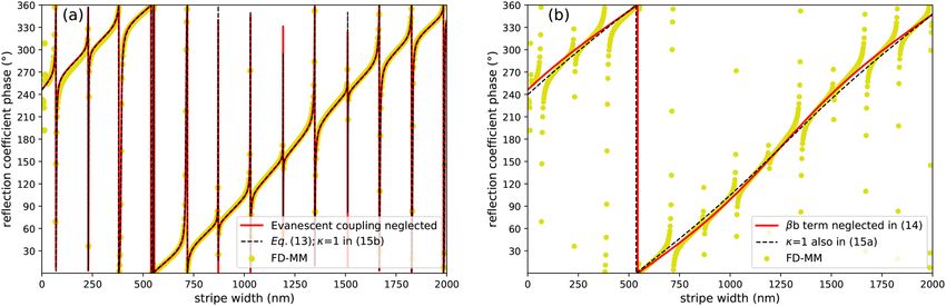
www.nature.com/scientificreports/
Figure 4. (a) Incident and reflected plane waves at an arbitrary time, and resulting interference pattern, in the
zero phase shift case, i.e., ϕ = 0◦. The dotted orange line and the dashed blue line correspond to the incident and
reflected plane waves, respectively. The solid green line corresponds to the interference pattern. (b) The same for
a phase shift of ϕ = 230◦, i.e., the value obtained for SW reflection from the edge of a semi-infinite 50-nm-thick
Py film.
Figure 5. (a) Phase shift of SWs at frequency 11 GHz as a function of the stripe width, calculated by the
FD-FEM. The stripe-film separation is s = 10 nm. Resonances (rapid changes of the phase shift, marked
with vertical dotted lines) appear periodically with a period of ca. 160 nm. (b) SW amplification factor in Py
below the stripe, obtained by dividing the maximum of |mx | in the part of the film lying below the stripe by
the maximum of |mx | in the far field. (c) Snapshot of the dynamic magnetization mx in a plateau region (stripe
width: 1270 nm). (d) Snapshot of the system in resonance at 11 GHz (stripe width: 1350 nm). The distance
between the red dashed lines in (c,d) corresponds to the SW wavelength in a uniform Py film at the same
frequency.
Phase shift dependence on stripe width. The introduction of a stripe over the Py film edge locally
modifies the environment in which SWs propagate due to dynamic dipolar interactions between the film and
the stripe. In consequence, it influences also the phase shift of reflected waves. The variation of this phase shift
with a stripe width at frequency 11 GHz, calculated using FD-FEM, is plotted in Fig. 5a. In general, this phase
shift, defined according to Eq. (3) with the interface located at the left edge of the stripe, at x = 0, grows steadily
with stripe width, however with periodic jumps by 360◦. These jumps occur approximately every 160 nm and are
accompanied by an increase of the amplitude of SWs in the Py film underneath the stripe, as shown in Fig. 5b. In
fact, at these stripe widths SWs are amplified in the whole bilayer, indicating that a resonant mode of the bilayer
is excited. This can be seen by comparing snapshots of mx for stripes of width 1270 nm (slowly changing phase
shift) and 1350 nm (rapidly changing phase shift) presented in Fig. 5c,d, respectively.
In addition to the enhancement of SW amplitude in the bilayer, Fig. 5c shows that the SWs in the stripe
and in the underlying Py layer have approximately opposite phases. In view of the profiles of the fast and slow
modes shown in Fig. 2d–g, we conclude that the slow modes dominate at observed resonances. However, the
magnetization pattern in both layers is more complex than that of a typical standing wave composed of two
counter-propagating waves with the same wavelength. Indeed, as discussed in “Dispersion relation of bilayers”,
the bilayer modes have an asymmetric dispersion r elation30. For such a scenario, we can generalize the resonance
condition Eq. (2) to
(kl + kr )w + ϕl + ϕr = 2πn, n = 1, 2, . . . , (4)
where ku and kd are the wavenumbers of right- and left-propagating modes, and ϕl and ϕr are the phase shifts
occurring at the left and right interfaces of the stripe. For ku = kd = k and ϕr = ϕl this equation reduces to
Eq. (2). Substituting here the wavelengths of the slow modes of a bilayer with s = 10 nm given in “Dispersion
relation of bilayers”, we conclude that successive resonances should occur every 160 nm, which matches very
well with the results of FD-FEM calculations shown in Fig. 5.
We have cross-checked these results against micromagnetic simulations made with a finite damping coefficient
α = 0.0001, see Fig. 6a for phase-width relation and Fig. 6b for amplitude-width relation. Due to computational
demands, these have been performed for a narrower range of stripe widths, 0–490 nm, 1000–1650 nm, and
Scientific Reports | (2021) 11:4428 | https://doi.org/10.1038/s41598-021-83307-9 5
Vol.:(0123456789)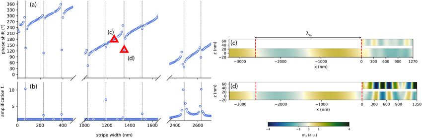
www.nature.com/scientificreports/
Figure 6. (a) Phase shift of SWs at frequency 11 GHz as a function of the stripe width obtained with
micromagnetic simulations. (b) SW amplification factor in Py below the stripe, defined as in Fig. 5b. (c)
Snapshot of the dynamic magnetization mx in a system without a resonance at 11 GHz (stripe width: 1270 nm).
(d) The same in a system possessing a resonance at 11 GHz (stripe width: 1350 nm). The distance between
the red dashed lines in (c,d) corresponds to the SW wavelength in a uniform Py film at the same frequency.
2350–2720 nm, encompassing several resonances. The obtained results are consistent with those of FD-FEM
calculations: the positions of resonances are the same as obtained by FD-FEM and the slope of the curve in
intermediate regions is virtually identical. The almost perfect alignment of those results obtained by two different
numerical methods confirms their correctness.
Snapshots of mx in systems with stripes of width 1270 nm and 1350 nm are displayed in Fig. 6c,d, respectively.
The former does not have a resonance at the chosen frequency, whereas the latter does. The obtained magnetiza-
tion patterns are qualitatively similar to those calculated by FD-FEM [Fig. 5c,d].
Two‑mode model analysis. The results presented above indicate that the bilayered part at the edge of the
semi-infinite ferromagnetic film allows an efficient control of the phase of the reflected SWs. The phase changes
rapidly when the width of the bilayered part fulfils the Fabry–Perot resonant condition, and thus the whole ele-
ment can be treated as a magnonic Gires–Tournois interferometer20. In this section we develop a detailed semi-
analytical model providing a clear justification and explanation of this process.
Wave scattering on the interface x = 0 separating the film and the bilayered part (see Fig. 1) can be described
by a scattering matrix S linking the complex amplitudes of the incoming and outgoing modes on both sides of the
interface. If both parts are sufficiently long for the amplitudes of all incoming evanescent modes to be negligible,
the amplitudes of the outgoing propagative modes are given by
d1 u1 S11 S12 S13 u1
u2 = S d2 ≡ S21 S22 S23 d2 . (5)
u3 d3 S31 S32 S33 d3
Here, u1 and d1 are the amplitudes of the right- and left-propagating modes of the Py film, u2 and d2 are the
amplitudes of the right- and left-propagating slow modes of the bilayer, and u3 and d3 are the amplitudes of
the right- and left-propagating fast modes of the bilayer (see the dispersion relation shown in Fig. 2). All these
amplitudes are measured at the interface between the film and the bilayer. The elements of the scattering matrix S
can be calculated using the finite-element modal method (see “Numerical methods”). At 11 GHz, their numeri-
cal values are
0.100 − 0.011i 0.135 + 0.016i 0.986 + 0.008i
S = −0.104 − 0.168i − 0.290 + 0.929i 0.035 − 0.113i (6)
0.975 − 0.023i 0.119 + 0.143i − 0.118 − 0.0273i
(these values are obtained for modes normalized to carry unit power, with the phase at the interface chosen so
that mx is real and positive on the symmetry axis of the Py layer). It can be seen that the film mode is coupled
primarily with the fast mode of the bilayer. The slow bilayer mode is strongly reflected. There is only weak, though
non-negligible, coupling between the fast and slow bilayer modes.
Likewise, the interface x = w between the bilayer and the vacuum can be described by a scattering matrix S′:
′
′
′
S S′
′
d2 u u2
′ = S′ ′ 2 ≡ ′ 22 ′ 23 . (7)
d3 u3 S 32 S 33 u′ 3
Here, u′ 2 and d ′ 2 are the amplitudes of the right- and left-propagating slow modes of the bilayer, and u′ 3 and d ′ 3
are the amplitudes of the right- and left-propagating fast modes of the bilayer, all measured at the bilayer-vacuum
interface (hence the prime, used to distinguish them from the amplitudes measured at the film-bilayer interface).
The numerical values of these scattering coefficients calculated at 11 GHz are
Scientific Reports | (2021) 11:4428 | https://doi.org/10.1038/s41598-021-83307-9 6
Vol:.(1234567890)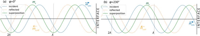
www.nature.com/scientificreports/


                                                                                  −0.043 + 0.975i − 0.103 + 0.190i
                                                                          S′ =                                       .                                         (8)
                                                                                   0.189 + 0.105i − 0.561 − 0.799i

                                  Both modes are strongly reflected and there is only weak cross-coupling.
                                     Mode amplitudes at the two interfaces are linked by
                                                                                   u′ i = exp(ikiu w) ui ≡ �iu ui ,                                           (9a)

                                                                          di = exp(−ikid w) d ′ i ≡ �id d ′ i ,         i = 2, 3,                             (9b)
                                  where kiu and kid are the wave numbers of the right- and left-propagating modes, numerically determined to be
                                 k2u = 16.2, k3u = 2.22, k2d = −23.1 and k3d = −1.90 rad/µm.
                                    Together, Eq. (5), Eq. (7) and Eq. (9) form a system of nine equations for as many unknown mode amplitudes
                                 (the amplitude u1 of the mode incident from the input film is treated as known). To obtain an intelligible expres-
                                 sion for the reflection coefficient r ≡ d1 /u1, it is advantageous to start by eliminating the amplitudes u3, d3, u′ 3
                                 and d ′ 3 of the fast bilayer mode, which is only weakly reflected at the interface with the Py film and hence will
                                 not give rise to strong Fabry–Perot-like resonances. This mimics the approach taken by Lecamp et al.31 in their
                                 model of pillar microcavities. This procedure reduces the second row of Eq. (5) and the first row of Eq. (7) to
                                                                                        u2 = S̃21 u1 + S̃22 d2 ,                                            (10a)

                                                                                  d ′ 2 = S̃′ 22 u′ 2 + S̃′ 23 3u S31 u1 ,                                 (10b)
                                  where
                                                                     1
                                                                                    S21 + κS23 �3d S′ 33 �3u S31 S22 + κS23 �3d S′ 33 �3u S32 ,

                                              S̃21 S̃22 ≡                                                                                                   (11a)
                                                            1 − κS23 �3d S′ 32 �2u

                                                                                     1            ′
                                                                                                  S 22 + κS′ 23 �3u S33 �3d S′ 32 αS′ 23
                                                         ′
                                                         S̃ 22 S̃′ 23 ≡

                                                                                                                                                            (11b)
                                                                          1 − κS′ 23 �3u S32 �2d
                                  and

                                                                                   κ ≡ (1 − S33 �3d S′ 33 �3u )−1 .                                           (12)
                                 The fast bilayer mode is only weakly reflected at the interface with the film: |S33 | ≈ 0.12 ≪ 1. Therefore multiple
                                 reflections of the fast mode at bilayer interfaces do not give rise to strong Fabry–Perot resonances and the coef-
                                 ficient κ remains close to 1 for all bilayer lengths. Together with the fact that the cross-coupling coefficients S23,
                                 S32, S′ 23 and S′ 32 are small, this means we can expect the scattering coefficients with a tilde defined in Eq. (11)
                                 to be well approximated by
                                                                                        S21 + S23 3d S′ 33 3u S31 S22

                                                                        S̃21 S̃22
                                                                                      ≈
                                                                                                  S′ 22             S′ 23
                                                                                                                            .                     (13)
                                                                       S̃′ 22 S̃′ 23
                                  Solving the equations remaining after elimination of the amplitudes of the fast mode for the amplitudes of the
                                  slow mode and substituting the resulting expressions to the formula for d1 in the first row in Eq. (5), we arrive
                                  at the following formula for the reflection coefficient:
                                                                                      r ≡ d1 /u1 = (a + βb),                                                  (14)
                                  where
                                                                                  a ≡ S11 + S13 �3d κS′ 33 �3u S31 ,                                        (15a)

                                          b ≡ S12 �2d (S̃′ 22 �2u S̃21 + S̃′ 23 �3u S31 )
                                                                                                                                                             (15b)
                                             + S13 �3d κ S′ 33 �3u S32 �2d (S̃′ 22 �2u S̃21 + S̃′ 23 �3u S31 ) + S′ 32 �2u (S̃21 + S̃22 �2d S̃′ 23 �3u S31 )


                                  and β represents the effect of multiple reflections of the slow mode:

                                                                                   β ≡ (1 − S22 �2d S′ 22 �2u )−1 .                                           (16)
                                  To facilitate the interpretation of Eqs. (14)–(16), the scattering coefficients with magnitude much smaller than 1
                                  have been underlined.
                                      It can be seen that the reflection coefficient r is made up of two terms. The first, a, is dominated by the phase
                                  shift acquired by the fast mode of the bilayer during a single round-trip across it. This term produces the slow
                                  but steady increase of the phase shift visible in Fig. 5a (also in Fig. 7). The second term, βb, is proportional to
                                  b, which is a superposition of six small terms, each containing a product of two scattering coefficients of small
                                  magnitude. Therefore βb has an appreciable effect on the reflection coefficient b only when the factor β , repre-
                                  senting the combined effect of multiple reflections of the slow mode on both ends of the bilayer, is much greater
                                  than 1. This happens at stripe widths w corresponding to Fabry–Perot resonances of the slow mode, where

Scientific Reports |   (2021) 11:4428 |                  https://doi.org/10.1038/s41598-021-83307-9                                                              7

                                                                                                                                                           Vol.:(0123456789)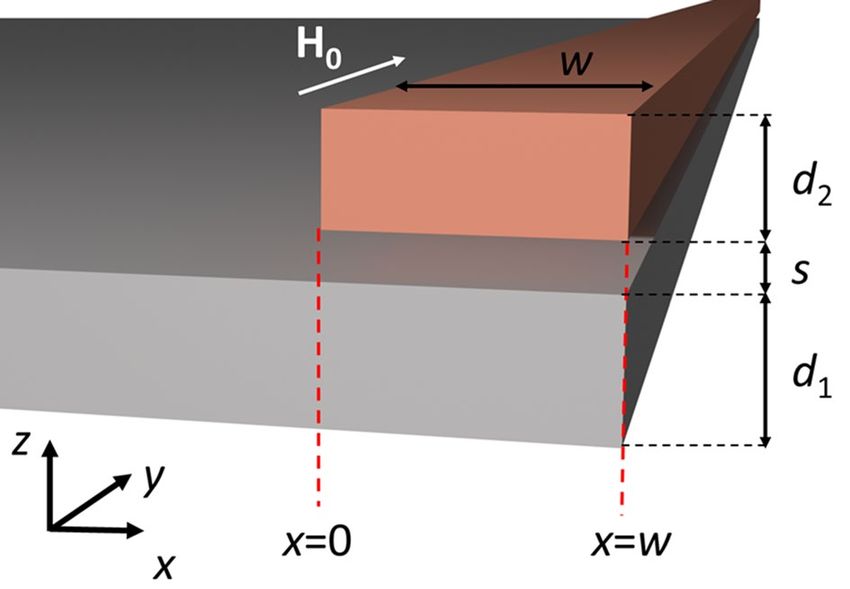
www.nature.com/scientificreports/

                                            Figure 7.  Comparison of the reflection coefficient phase calculated numerically using the finite-element modal
                                            method FD-MM (points) with the semi-analytical model from Eq. (14) at varying degrees of approximation
                                            (lines). Details in the plot legends and in the text.

                                            Figure 8.  (a) Phase shift dependence on the separation between the FM2 stripe and Py film, calculated
                                            by the FD-FEM. (b–e) Snapshots of the dynamic magnetization mx at separations 10, 28, 50 and 106 nm,
                                            corresponding to the resonances marked in plot (a). The dashed red lines mark the SW wavelength in the Py
                                            film. (f) Red line: dependence of the resonance index n calculated from Eq. (4) on the separation s, with ϕl + ϕr
                                            set to the fitted value 0.12. Resonances are predicted to occur at integer values of n. Black circles: positions of
                                            resonances found in FD-FEM calculations.

                                           [arg S22 + arg S′ 22 + (k2u + k2d )w] is a multiple of 2π , justifying the postulated resonance condition Eq. (4).
                                           Since b is a combination of multiple terms of similar magnitude, its dependence on the stripe width is rather
                                           complicated. This explains the variability of the shapes of individual resonances in Fig. 5a (also in Fig. 7a).
                                               To confirm this interpretation of the role of the various terms in Eq. (14), let us visualize and compare
                                           the effects of applying successively stronger approximations to it. In Fig. 7a,b, the golden symbols show the
                                           variation of the phase of the reflection coefficient obtained directly from numerical calculations made with the
                                           finite-element modal method (in close agreement with the FD-FEM results from Fig. 5a). The red solid curve
                                           in Fig. 7a shows the phase of the reflection coefficient calculated from Eq. (14). The only approximation made
                                           in its derivation was to neglect evanescent coupling between the left and right end of the bilayer; clearly, this
                                           approximation is very well satisfied everywhere except for stripes narrower than 250 nm. The black dashed curve
                                           in Fig. 7a shows the effect of applying the approximation Eq. (13) and setting κ to 1 in the formula Eq. (15b)
                                           for b (but not in the formula Eq. (15a) for a). This corresponds to neglecting terms proportional to products of
                                           more than two small scattering coefficients; the resulting curve is almost indistinguishable from the previous
                                           one. Neglecting the second term βb in Eq. (14) produces the red solid curve in Fig. 7b. The resonances are gone,
                                           but the long-term increase in phase shift with stripe width is still reproduced faithfully. Finally, the black dashed
                                           curve in Fig. 7b shows the result of approximating κ by 1 also in the formula Eq. (15a) for a. Its small deviation
                                           from the red curve confirms the minor role played by multiple reflections of the fast mode.

          Scientific Reports |   (2021) 11:4428 |                https://doi.org/10.1038/s41598-021-83307-9                                                       8

Vol:.(1234567890)
www.nature.com/scientificreports/
Phase shift dependence on the layer separation. In “Dispersion relation of bilayers” we observed
that the separation influences the strength of the dynamical dipolar coupling between the infinitely wide stripe
and Py film. It affects the SW dispersion relation, especially the wavelengths of the slow modes propagating
leftwards and rightwards. Therefore, according to Eq. (4), by varying the separation s, and hence ku and kd , while
keeping the stripe width w constant, it should be possible to sweep over resonances of different orders n. Indeed,
we have found multiple resonances in dependence of the phase shift on the separation s, for a stripe of width
w = 1676 nm, as shown in Fig. 8a.
Resonances do not appear periodically; the spacing between subsequent Fabry–Perot resonances increases
with the altitude of the stripe, and for the chosen stripe width the last resonance occurs at the separation
s = 106 nm. This is because with increasing s the coupling between the Py film and the stripe weakens and the
wavenumbers ku and kd approach their asymptotic limits. Snapshots of the magnetization at the resonances found
at separations 10, 28, 50 and 106 nm are shown in Fig. 8b–e. These figures demonstrate a clear enhancement of
the SW amplitude below the stripe and a decrease in the number of nodal point with increasing separation, in
line with the shift of the dispersion relation of the slow mode towards smaller wavenumbers shown in Fig. 2c.
Combining the Fabry–Perot resonance condition, Eq. (4), with the numerically calculated dispersion rela-
tions and setting ϕl + ϕr to the fitted value of 0.12, we calculate the dependence of n on the separation between
the stripe and the Py film, plotted with the red line in Fig. 8f. In the range from 106 down to 5 nm, we find six
integer values of n, corresponding to successive resonances. These values agree well with the results of FD-FEM
calculations, where six resonances, marked with black points in Fig. 8f, are detected in that range of separation.
Conclusions
We have studied theoretically the influence of a narrow ferromagnetic stripe of subwavelength width placed at
the edge of a ferromagnetic film on the phase of reflected SWs. At the considered frequency (11 GHz) the bilayer
formed by the film and the stripe supports two pairs of slow (short wavelength) and fast (long wavelength) guided
SW modes propagating in opposite directions; these modes couple with the SW mode of the Py film. This allowed
us to interpret the numerical results by modelling the system as a series of waveguides linked by junctions at
which waveguide modes are scattered into each other.
We have found a strong nonlinear dependence of the phase shift on the stripe width. In particular, we
have shown that the reflection coefficient, from which the phase shift can be derived, consists of two terms,
each having a different origin. One produces a slow but steady increase of the phase shift with increasing bilayer
width and is dominated by the phase accumulated by the fast mode during a single round-trip across the bilayer.
The other term has an appreciable effect on the reflection coefficient only when multiple reflections of the slow
mode on both edges of the bilayer interfere constructively, which corresponds to Fabry–Perot resonances of
this mode. Interestingly, the incoming wave from the Py film couples strongly only to the fast mode, but at
Fabry–Perot resonances, the phase of the reflected SW is controlled by the slow mode only weakly coupled to
the propagating wave and to the fast mode of the bilayer. Essentially, this system is a realization of a Gires–Tour-
nois interferometer20 operating on SWs. However, in our design, its width is smaller than the wavelength of the
incident wave and the interferometer utilizes two nonreciprocal SW modes present in the bilayer, thus offering
further prospects for the design of subwavelength resonant elements with nonreciprocal properties for SW phase
control and development of magnon logic.
We have also found that the phase shift of the reflected SW passes through a series of resonances as the sepa-
ration between the stripe and the Py film is increased. This unexpected effect originates from the dependence of
the wavelength of the slow SW in the bilayer on the strength of the dipolar coupling between the two layers. As
a result, the bilayer width at which the Fabry–Perot condition is satisfied changes with the coupling strength as
well, giving rise to the separation-dependent resonances. Increasing the stripe-film separation by 1 nm produces
a 360-degree shift of the phase of the reflected wave; this high sensitivity is favorable for sensing applications.
Overall, this research shows that SW Gires–Tournois interferometer can be used to modify the phase of
reflected SWs in a wide range by tiny changes of the bilayer part width or stripe-film distance. This is significant
for the further development of magnonic devices where SW phase control is of key importance, in particular
in integrated systems with components smaller than the SW wavelength. This may include the use of arrays of
resonators in tunable SW optical elements, such as lenses, magnonic metasurfaces and phase shifters, as well
as the sensing applications of magnonics, for example the development of magnonic counterparts of sensors
utilizing surface plasmon resonances.
Methods
Governing equations. The magnetization dynamics is described by the Landau-Lifshitz equation:
|γ |µ0 α
∂t M = − M × H eff + M × (M × H eff ,
) (17)
1 + α2 MS
where M is the magnetization vector, µ0 is the permeability of vacuum, α is a dimensionless damping parameter,
and Heff = H0 + HM + Hex is the effective magnetic field. The latter is the sum of the external magnetic field
H0, the magnetostatic field HM, and the isotropic Heisenberg exchange field Hex = ∇ · (l 2 ∇M).
The magnetostatic field fulfils the magnetostatic Maxwell’s equations
∇ · (M + HM ) = 0, (18a)
∇ × HM = 0; (18b)
Scientific Reports | (2021) 11:4428 | https://doi.org/10.1038/s41598-021-83307-9 9
Vol.:(0123456789)www.nature.com/scientificreports/
the latter makes it possible to write it as HM = −∇ϕ , where ϕ is the magnetic scalar potential.
Assuming a harmonic time dependence [exp(−iωt )], zero damping ( α = 0) and alignment of the external
magnetic field H0 with the y axis, splitting the magnetization M and magnetostatic field HM into static ( MS ŷ, H0 ŷ )
and dynamic (radio-frequency) components (m = [mx , 0, mz ], hM = [−∂x ϕ, 0, −∂z ϕ]), linearizing the Landau-
Lifshitz equation (17) (applicable only in the ferromagnetic layers) and coupling it with the Gauss law for
magnetism, Eq. (18a) (applicable everywhere), we arrive at the following system of equations for the magnetic
potential ϕ and the dynamic magnetization component m:
∂x (mx − ∂x ϕ) + ∂z (mz − ∂z ϕ) = 0, (19a)
H0 iω
∂x ϕ − ∇ · (l 2 ∇mx ) + mx − mz = 0, (19b)
MS |γ |µ0 MS
H0 iω
∂z ϕ − ∇ · (l 2 ∇mz ) + mz + mx = 0. (19c)
MS |γ |µ0 MS
Numerical methods. We have used three complementary numerical methods to study SW dynamics.
First, we use micromagnetic simulations performed in the open-source mumax3 e nvironment32, which solves
the full Landau-Lifshitz equation [Eq. (17)] with the finite-difference time-domain (FDTD) method. We use this
method to calculate the dispersion relations of SWs and steady states obtainable after long continuous excitation
of SWs by a specified source. Micromagnetic simulations were performed for magnetic parameters and geom-
etry described in “Structure under consideration” and damping α = 0.0001. The simulated structure was discre-
tized with a mesh consisting of regular 5 × 100 × 5 nm3 (along the x, y, z axis) unit cells. In order to model a film
infinitely extended along the y axis, we imposed periodic boundary conditions along the y axis with assumed
1024 repetitions of the system along this axis. After stabilizing the system with a magnetic field of value 0.1 T
applied along the y axis, SWs were excited in the film by a local source of microwave-frequency magnetic field of
frequency 11 GHz and amplitude 0.1 mT placed at 3.6 µm from the right edge. To prevent wave reflections from
the left edge of the film, an absorbing zone with gradually increasing damping was defined on the left side of
the system. A continuous harmonic SW excitation was maintained for 162.6 ns in order to reach a fully evolved
(steady-state) interference pattern of the incident and reflected waves. The main disadvantage of this method is
its high computational cost. Resonant systems can take a long time to reach steady state, and the cost of a single
time step is pushed up by the need to discretize the whole system on a uniform grid whose resolution is dictated
by the size of the smallest geometric features.
In order to avoid these limitations, we rely primarily on calculations using the frequency-domain finite ele-
ment method (FD-FEM). Its major advantage is the possibility of refining the mesh locally, e.g. only around small
geometric features, rather than globally. In addition, it allows direct and fast calculation of the eigenfrequencies
and eigenmodes (mode profiles) of the system, which can be identified with its steady states. To perform the
calculations, we have used the COMSOL Multiphysics s oftware33 to solve the linearized Landau-Lifshitz equa-
tion coupled with the Gauss law, Eqs. (19), as described in Refs.34,35. At the edges of the computational domain
(far from the ferromagnetic materials) the Dirichlet boundary conditions, forcing the magnetic potential to
vanish, are imposed.
In “Two-mode model analysis” we have formulated a semi-analytical model dependent on the numerical
values of scattering matrices associated with interfaces separating parts of the system with different cross-sections.
Calculation of these matrices with the methods mentioned above is cumbersome and produces results of rela-
tively low accuracy. The scattering matrices must be obtained by fitting superpositions of complex exponentials
to calculated field distributions; the results are affected by the presence of evanescent fields near material discon-
tinuities and by spurious reflections from boundaries of the computational domain. Therefore we calculate the
scattering matrices using a finite-element modal method; this technique, inspired by similar approaches used
in photonics36 will be described in detail in a forthcoming paper37. In essence, we proceed in two steps. First,
Eq. (19) describing each x-invariant part of the system (a SW waveguide with a fixed cross-section) is trans-
formed into an eigenproblem whose solutions are the wavenumbers and profiles of propagative and evanescent
modes of that waveguide. This problem is then discretized by expanding the magnetic potential and dynamic
magnetization profile in a finite-element basis and solved numerically. Second, fields in each x-invariant section
are represented as a superposition of the eigenmodes calculated in the previous step. Imposition of the standard
continuity conditions on the interface separating a pair of adjacent sections leads to a linear system whose solu-
tion yields the scattering matrix linking the complex amplitudes of modes impinging onto the interface with the
amplitudes of outgoing modes. The scattering matrices of individual interfaces and finite-length sections can then
be concatenated together using standard a lgorithms38 to produce the scattering matrix of the complete system.
In contrast to the previous two methods, the modal method produces results unaffected by spurious reflections
from boundaries truncating the computational domain along x, since the radiation conditions at x − → ±∞ are
fulfilled analytically. In addition, no fitting is required to obtain the scattering coefficients.
Received: 3 December 2020; Accepted: 25 January 2021
References
1. Ng, I. C. & Wakenshaw, S. Y. The internet-of-things: Review and research directions. Int. J. Res. Mark. 34, 3–21 (2017).
Scientific Reports | (2021) 11:4428 | https://doi.org/10.1038/s41598-021-83307-9 10
Vol:.(1234567890)www.nature.com/scientificreports/
2. Krawczyk, M. & Grundler, D. Review and prospects of magnonic crystals and devices with reprogrammable band structure. J.
Phys. Condens. Matter 26, 123202 (2014).
3. Chumak, A., Vasyuchka, V., Serga, A. & Hillebrands, B. Magnon spintronics. Nat. Phys. 11, 453–461 (2015).
4. Chumak, A. V. Fundamentals of magnon-based computing. arXiv preprint arXiv:1901.08934 (2019).
5. Yu, N. & Capasso, F. Flat optics with designer metasurfaces. Nat. Mater. 13, 139–150 (2014).
6. Yu, N. et al. Light propagation with phase discontinuities: Generalized laws of reflection and refraction. Science 334, 333–337
(2011).
7. Kumar, K. et al. Printing colour at the optical diffraction limit. Nat. Nanotechnol. 7, 557 (2012).
8. Vashistha, V., Vaidya, G., Gruszecki, P., Serebryannikov, A. E. & Krawczyk, M. Polarization tunable all-dielectric color filters based
on cross-shaped Si nanoantennas. Sci. Rep. 7, 8092 (2017).
9. Kruglyak, V. et al. Graded magnonic index and spin wave Fano resonances in magnetic structures: Excite, direct, capture. in Spin
Wave Confinement - Propagating Waves, 2nd edn (eds Demokritov, S. O.) (Jenny Stanford Publishing, Boca Raton, 2017).
10. Au, Y., Dvornik, M., Dmytriiev, O. & Kruglyak, V. Nanoscale spin wave valve and phase shifter. Appl. Phys. Lett. 100, 172408 (2012).
11. Au, Y. et al. Resonant microwave-to-spin-wave transducer. Appl. Phys. Lett. 100, 182404 (2012).
12. Yu, T., Blanter, Y. M. & Bauer, G. E. Chiral pumping of spin waves. Phys. Rev. Lett. 123, 247202 (2019).
13. Yu, T., Liu, C., Yu, H., Blanter, Y. M. & Bauer, G. E. Chiral excitation of spin waves in ferromagnetic films by magnetic nanowire
gratings. Phys. Rev. B 99, 134424 (2019).
14. Al-Wahsh, H. et al. Evidence of Fano-like resonances in mono-mode magnetic circuits. Phys. Rev. B 78, 075401 (2008).
15. Zhang, Z. et al. Bias-free reconfigurable magnonic phase shifter based on a spin-current controlled ferromagnetic resonator. J.
Phys. D 53, 105002 (2020).
16. Yu, H. et al. Omnidirectional spin-wave nanograting coupler. Nat. Commun. 4, 2702 (2013).
17. Yu, H. et al. Approaching soft x-ray wavelengths in nanomagnet-based microwave technology. Nat. Commun. 7, 11255 (2016).
18. Graczyk, P. et al. Magnonic band gap and mode hybridization in continuous permalloy films induced by vertical dynamic coupling
with an array of permalloy ellipses. Phys. Rev. B 98, 174420 (2018).
19. Mieszczak, S. et al. Anomalous refraction of spin waves as a way to guide signals in curved magnonic multimode waveguides.
Phys. Rev. Appl. 13, 054038 (2020).
20. Gires, F. & Tournois, P. Interferometre utilisable pour la compression d’impulsions lumineuses modulées en frequence. C. R. Acad.
Sci. Paris. 258, 6112–6115 (1964).
21. Stancil, D. D. & Prabhakar, A. Spin waves: Theory and applications (Springer, Berlin, 2009).
22. Gurevich, A. G. & Melkov, G. A. Magnetization Oscillations and Waves (CRC Press, Boca Raton, 1996).
23. Mruczkiewicz, M. & Krawczyk, M. Nonreciprocal dispersion of spin waves in ferromagnetic thin films covered with a finite-
conductivity metal. J. Appl. Phys. 115, 113909 (2014).
24. Gallardo, R. et al. Reconfigurable spin-wave nonreciprocity induced by dipolar interaction in a coupled ferromagnetic bilayer.
Phys. Rev. Appl. 12, 034012 (2019).
25. An, K., Bhat, V., Mruczkiewicz, M., Dubs, C. & Grundler, D. Optimization of spin-wave propagation with enhanced group veloci-
ties by exchange-coupled ferrimagnet-ferromagnet bilayers. Phys. Rev. Appl. 11, 034065 (2019).
26. Guslienko, K. Y., Demokritov, S. O., Hillebrands, B. & Slavin, A. N. Effective dipolar boundary conditions for dynamic magnetiza-
tion in thin magnetic stripes. Phys. Rev. B 66, 132402 (2002).
27. Centała, G. et al. Influence of nonmagnetic dielectric spacers on the spin-wave response of one-dimensional planar magnonic
crystals. Phys. Rev. B 100, 224428 (2019).
28. Stigloher, J. et al. Observation of a Goos-Hänchen-like phase shift for magnetostatic spin waves. Phys. Rev. Lett. 121, 137201 (2018).
29. Verba, R., Tiberkevich, V. & Slavin, A. Spin-wave transmission through an internal boundary: Beyond the scalar approximation.
Phys. Rev. B 101, 144430 (2020).
30. Zingsem, B. W., Farle, M., Stamps, R. L. & Camley, R. E. Unusual nature of confined modes in a chiral system: Directional transport
in standing waves. Phys. Rev. B 99, 214429 (2019).
31. Lecamp, G., Lalanne, P., Hugonin, J. P. & Gerard, J.-M. Energy transfer through laterally confined Bragg mirrors and its impact
on pillar microcavities. IEEE J. Quant. Electron. 41, 1323–1329 (2005).
32. Vansteenkiste, A. et al. The design and verification of mumax3. AIP Adv. 4, 107133 (2014).
33. COMSOL Multiphysics 5.1a, www.comsol.com, COMSOL AB, Stockholm, Sweden.
34. Rychły, J. & Kłos, J. W. Spin wave surface states in 1D planar magnonic crystals. J. Phys. D: Appl. Phys. 50, 164004 (2017).
35. Graczyk, P., Zelent, M. & Krawczyk, M. Co-and contra-directional vertical coupling between ferromagnetic layers with grating
for short-wavelength spin wave generation. New J. Phys. 20, 053021 (2018).
36. Liu, Q.-H. & Chew, W. C. Numerical mode-matching method for the multiregion vertically stratified media. IEEE Trans. Antennas
Propag. 38, 498–506 (1990).
37. Śmigaj, W., Sobucki, K., Gruszecki, P. & Krawczyk, M. In preparation.
38. Li, L. Formulation and comparison of two recursive matrix algorithms for modeling layered diffraction gratings. J. Opt. Soc. Am.
A 13, 1024–1035 (1996).
Acknowledgements
The research leading to these results has received funding from the Polish National Science Centre projects No.
UMO-2015/17/B/ST3/00118, UMO-2019/33/B/ST5/02013, and UMO-2019/35/D/ST3/03729. J.R. acknowledges
the financial support of the National Science Centre Poland under the decision DEC-2018/30/E/ST3/00267. The
simulations were partially performed at the Poznan Supercomputing and Networking Center (Grant No. 398).
Author contributions
K.S. performed frequency-domain finite-element and finite-difference time-domain simulations of the reflection
of spin waves and processed the data. W.Ś. formulated the two-mode model and performed calculations with
the finite-element modal method. J.R. and P.G. computed dispersion relations. K.S. and P.G. prepared figures.
P.G. and M.K. supervised the study. All authors analysed the results and contributed to writing the manuscript.
Competing interests
The authors declare no competing interests.
Additional information
Correspondence and requests for materials should be addressed to K.S. or P.G.
Reprints and permissions information is available at www.nature.com/reprints.
Scientific Reports | (2021) 11:4428 | https://doi.org/10.1038/s41598-021-83307-9 11
Vol.:(0123456789)www.nature.com/scientificreports/
Publisher’s note Springer Nature remains neutral with regard to jurisdictional claims in published maps and
institutional affiliations.
Open Access This article is licensed under a Creative Commons Attribution 4.0 International
License, which permits use, sharing, adaptation, distribution and reproduction in any medium or
format, as long as you give appropriate credit to the original author(s) and the source, provide a link to the
Creative Commons licence, and indicate if changes were made. The images or other third party material in this
article are included in the article’s Creative Commons licence, unless indicated otherwise in a credit line to the
material. If material is not included in the article’s Creative Commons licence and your intended use is not
permitted by statutory regulation or exceeds the permitted use, you will need to obtain permission directly from
the copyright holder. To view a copy of this licence, visit http://creativecommons.org/licenses/by/4.0/.
© The Author(s) 2021
Scientific Reports | (2021) 11:4428 | https://doi.org/10.1038/s41598-021-83307-9 12
Vol:.(1234567890)You can also read