Modeling the annual cycle of daily Antarctic sea ice extent
←
→
Page content transcription
If your browser does not render page correctly, please read the page content below
The Cryosphere, 14, 2159–2172, 2020
https://doi.org/10.5194/tc-14-2159-2020
© Author(s) 2020. This work is distributed under
the Creative Commons Attribution 4.0 License.

Modeling the annual cycle of daily Antarctic sea ice extent
Mark S. Handcock1 and Marilyn N. Raphael2
1 Department   of Statistics, University of California, Los Angeles, USA
2 Department   of Geography, University of California, Los Angeles, USA

Correspondence: Mark S. Handcock (handcock@stat.ucla.edu)

Received: 29 August 2019 – Discussion started: 29 October 2019
Revised: 8 April 2020 – Accepted: 6 May 2020 – Published: 2 July 2020

Abstract. The total Antarctic sea ice extent (SIE) experi-        1   Introduction
ences a distinct annual cycle, peaking in September and
reaching its minimum in February. In this paper we propose        Much of the research on Antarctic sea ice variability focuses
a mathematical and statistical decomposition of this temporal     on the monthly, seasonal and interannual timescales (Parkin-
variation in SIE. Each component is interpretable and, when       son and Cavalieri, 2012; Simpkins et al., 2012; Holland,
combined, gives a complete picture of the variation in the sea    2014; Turner et al., 2015b; Hobbs et al., 2015; Holland et al.,
ice. We consider timescales varying from the instantaneous        2017). This is useful and necessary, especially if links to the
and not previously defined to the multi-decadal curvilinear       larger-scale (and remote) atmospheric and oceanic forcings
trend, the longest. Because our representation is daily, these    are to be made. However, significant aspects of the timing of
timescales of variability give precise information about the      the ice cycle, for example when ice advance or ice retreat be-
timing and rates of advance and retreat of the ice and may        gins, occur at sub-monthly scales (Stammerjohn et al., 2008;
be used to diagnose physical contributors to variability in the   Stuecker et al., 2017; Turner et al., 2017; Schlosser et al.,
sea ice. We define a number of annual cycles each captur-         2018; Meehl et al., 2019). Using daily data facilitates analy-
ing different components of variation, especially the yearly      sis of the daily variation in sea ice and is the springboard of
amplitude and phase that are major contributors to SIE vari-      this research.
ation. Using daily sea ice concentration data, we show that          The dominant or primary characteristic of Antarctic sea ice
our proposed invariant annual cycle explains 29 % more of         variability is its annual cycle. Satellite-observed total Antarc-
the variation in daily SIE than the traditional method. The       tic sea ice extent (SIE) experiences a distinct annual cycle,
proposed annual cycle that incorporates amplitude and phase       peaking in September (19 million km2 ) and reaching its min-
variation explains 77 % more variation than the traditional       imum in February (3 million km2 ) on average. In Julian days,
method. The variation in phase explains more of the variabil-     the median minimum day is 50 and the median maximum
ity in SIE than the amplitude. Using our methodology, we          day is 255. The growth from minimum (trough) to maximum
show that the anomalous decay of sea ice in 2016 was asso-        (peak) is slower than the retreat from maximum to minimum.
ciated largely with a change of phase rather than amplitude.      This is arguably the strongest seasonal cycle on the planet.
We show that the long term trend in Antarctic sea ice extent      The characteristics of the annual cycle that are of major inter-
is strongly curvilinear and the reported positive linear trend    est are its amplitude and its phase. The amplitude is consid-
is small and dependent strongly on a positive trend that began    ered to be the difference between SIE at maximum and SIE
around 2011 and continued until 2016.                             at minimum. The phase is the timing of advance and retreat
                                                                  of the ice with respect to the typical annual cycle. In recent
                                                                  years the sensitivity of the amplitude and phase to climate
                                                                  change has been the subject of much study (e.g., Stammer-
                                                                  john et al., 2008; Turner et al., 2017; Turner et al., 2015a;
                                                                  Parkinson, 2019).

Published by Copernicus Publications on behalf of the European Geosciences Union.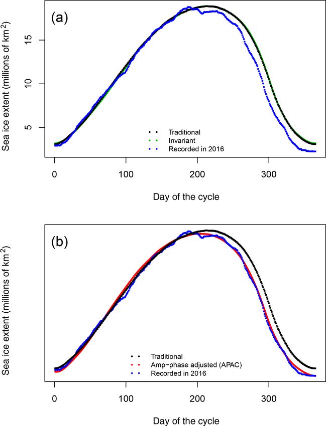
2160 M. S. Handcock and M. N. Raphael: Modeling the annual cycle
The daily, annual cycle of SIE is traditionally calculated a pattern that allows both temporal dilation and contraction
by simply taking the average (or the median value) for each as well as amplitude modulation.
day of the year. However, satellite-observed SIE can vary To show the utility of the model, we develop several dif-
widely from day to day. Some of this variation is due to the ferent annual cycles, including one that is invariant, one that
ice growth, melting, and divergence of the ice at the ice edge is adjusted for phase only and one that is adjusted for am-
and land spillover (coastal effect of mixed land/water grid plitude only. From the modeled annual cycles we define and
cells), while some is due, for example, to transient effects extract the variability at the timescales mentioned. We con-
of cloud and melt on the ice surface (e.g., Comiso and Stef- clude with a decomposition of the variability of SIE during
fen, 2001). A simple daily average or median includes all 2016, the year of anomalous decay of SIE. The data are de-
of these sources of variability, perhaps leading to overesti- scribed in Sect. 2, and the model is defined and developed in
mation or underestimation of the SIE. Therefore, a standard Sect. 3. The results are presented and discussed in Sect. 3,
deviation (or a percentile) is often included to give some idea while conclusions are made in Sect. 4.
of the variability of the individual days around the mean for
that day. While simple and transparent, this method of cal-
culating the annual cycle produces a value that is subject to 2 Data
substantial variation since it is based on as few as 40 numbers
We used the Bootstrap Version 3 concentration fields
(the length of the satellite-observed data time series), one for
(Comiso, 2017) from the NOAA/NSIDC Climate Data
each year of recorded data, and does not include the effect of
Record of Passive Microwave Sea Ice Concentration, Ver-
the day preceding or the day following the averaged day. It
sion 3 (Peng et al., 2013; Meier et al., 2017). These data
is also influenced by the pattern of missing values. Finally,
were generated using the Advanced Microwave Scanning
it also disguises the fact that the daily annual cycle might be
Radiometer – Earth Observing System (AMSR-E) Bootstrap
slowly changing phase and that the amplitude and shape of
Algorithm with daily varying tie points. They span the pe-
the daily annual cycle of SIE might vary. This can make it
riod 26 October 1978 to 31 December 2018 and are daily
difficult to make statistically sound conclusions about vari-
except prior to July 1987 when they are given every other
ability in the data.
day. Data are gridded on the SSM/I polar stereographic grid
Our overarching aim in this research is not only to redefine
(25 km× 25 km). In addition to the alternate day observations
the annual cycle but also to make a meaningful decomposi-
from 1978 to 1987, there are a number of days and segments
tion of the variation in the annual cycle of Antarctic SIE. We
of days with no observations. In particular, there are no data
do so on the time dimension in such a way that each com-
between early December 1987 and mid-January 1988. Our
ponent can be interpreted individually, and when taken to-
methods do not require a complete temporal data record and
gether all of the components give a complete picture of the
naturally deal with missing data. As such we do not impute
variation in the sea ice. We consider the variation from the
the missing days. The SIE used in our analysis was calcu-
shortest timescale (instantaneous variation) and increasing
lated using the conventional limit of the 15 % SIC isoline.
the timescale sequentially we move through the day-to-day
Every grid poleward of the 15 % isoline is considered to be
variation, the year-to-year (interannual) variation, and finally
completely covered with ice.
the longest timescale, the curvilinear trends of the multi-
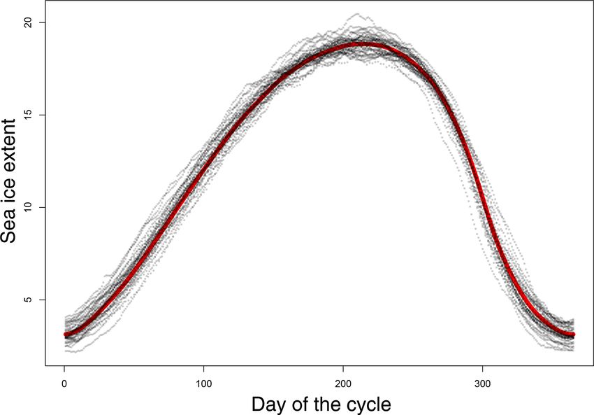
Figure 1 shows the recorded total SIE (in grey dots) for
decadal variation. In the process, we make a number of tech-
each year from 1979 to 2017 and a smoothed representation
nical contributions, most importantly to define complemen-
of the traditional daily annual cycle (red). In this figure, day 0
tary types of annual cycles that are meaningful in terms of
on the horizontal axis represents the typical lowest SIE for
this decomposition and also to the representation of volatil-
the year, Julian day 50. We employ this convention for all
ity. We have deliberately chosen (time) dimensions based on
of the time series figures used in this paper. The plot nicely
their interpretability rather than solely statistical efficiency
illustrates the variation in the SIE from day-to-day and year
concerns. For example, the amplitude and phase components
to year.
of the decomposition are much more interpretable than sim-
ple spectral components.
We begin by presenting a stochastic model for the sea ice 3 Methods and results: a statistical decomposition of
extent that allows the annual cycle to be defined in flexible sea ice extent
ways. This model can represent the real variability in SIE
and reduces the contribution from the ephemeral effects de- 3.1 Annual cycle definition
scribed above. The model can account for the fact that the
ice maximum is not achieved on the same day of the ice cy- In this section we give five ways to define an annual cycle
cle each year. It also recognizes that the length of the ice in the sea ice extent. We start with the traditional definition
cycle will vary and that the timing of advance and retreat of of the annual cycle and progressively define annual cycles
the ice varies from year to year. This means that the annual that are more sophisticated and that can represent more of
cycle is not constrained to a fixed cyclical pattern, rather it is the variation in the SIE over time. The second is an invariant
The Cryosphere, 14, 2159–2172, 2020 https://doi.org/10.5194/tc-14-2159-2020
M. S. Handcock and M. N. Raphael: Modeling the annual cycle                                                                        2161

Figure 1. Recorded sea ice extent (SIE) (grey) for each year compared to a smooth annual cycle (red) over a 365 d period. The horizontal
axis is the day of the cycle and the vertical axis is sea ice extent in millions of square kilometers.

annual cycle that retains the 365 d period of the traditional            Within this representation, the annual cycle is traditionally
but incorporates the smooth functional form we might ex-              estimated by aT [s]:
pect. The third adds amplitude variation to the invariant an-
                                                                                      1           X
nual cycle so that the cycle itself varies from year to year          aT [s] = P                          extent(t),
with the amplitude of the year. The fourth adds phase varia-                      t:doy(t)=s 1 t:doy(t)=s
tion to the invariant annual cycle, allowing it to capture the        where t = T0 , . . ., T ,                                       (2)
timing of the ice advance and retreat over each year. Finally,                P
the fifth adds both amplitude and phase variation to the in-          where t:doy(t)=s 1 = 40 is the number of years of data.
variant annual cycle, allowing it to represent variation over            This traditional estimate (aT [s],) has a number of statis-
time in both the amplitude and phase of the SIE.                      tical issues that reduce its utility for examining the sea ice
                                                                      variability. Firstly, it is typically based on data for a subset of
Traditional annual cycle                                              the satellite era (e.g., from 1979 onward). Currently, this is
                                                                      about 40 years of data, inducing intrinsic statistical variabil-
Our decomposition of the sea ice extent starts with the tradi-        ity into aT [s] as an estimate of a[s]. This could be reduced
tional representation based on the annual cycle is as follows:        by increasing the temporal range backward, by, for example,
                                                                      including data from the earlier satellite record (NIMBUS-5).
extent(t) = a[doy(t)] + α(t) where t = T0 , . . ., T ,        (1)     Another option is to include information from proxy sources.
                                                                      However, this requires a large and sophisticated model-based
where extent(t) is the extent on day t expressed as a decimal
                                                                      reconstruction and we do not consider such methods fur-
year (e.g., 1 February 2010 as 2010.08767) and doy(t) is the
                                                                      ther in this paper. Secondly, aT [s] is computed separately for
day of the year for t (e.g., 32). Most importantly, a is an
                                                                      each day, ignoring the surrounding days. There is informa-
annual cycle shape function with a(s) giving the annual cycle
                                                                      tion in the temporally close days in the intuitive sense that
shape value for day of the year s. In this context, α(t) is the
                                                                      days close to s, e.g., s − 1 and s + 1, will have similar, albeit
anomaly of the extent from the annual cycle on day t, T0 is
                                                                      not exactly the same, values. This information is ignored by
the first observed time and T is the last observed time. For
                                                                      aT [s]. Thirdly, we expect a[s] to be smooth as a function of
the data in this paper, T0 = 1978.833 and T = 2019.000.
                                                                      s so that changes in aT [s] with s will be similar for days that
                                                                      are close. Fourthly, we expect that aT [s] will “over fit” to
                                                                      the record, making the estimated anomalies from it smaller
                                                                      than the true anomaly, α(t), and that the annual cycle esti-

https://doi.org/10.5194/tc-14-2159-2020                                                      The Cryosphere, 14, 2159–2172, 2020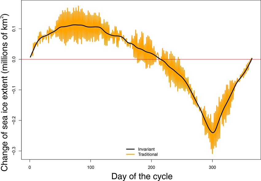
2162 M. S. Handcock and M. N. Raphael: Modeling the annual cycle
mates will be more variable than the true annual cycle. This Amplitude-adjusted annual cycle
last issue is induced by the finite record and the estimates
of the anomaly α̂(t) = extent(t) − aT [doy(t)] will be statisti- The invariant annual cycle has the same motivation as the tra-
cally different than those of α(t). In summary, the traditional ditional annual cycle while being a clear statistical and con-
estimate, aT [s], uses limited information, ignores other days, ceptual improvement over the traditional cycle. However, we
is not as smooth as we expect due to day-to-day variation, argue that since it is also fixed by day of year, it may be
and over fits to the record. too restrictive since it, like the traditional cycle, disguises the
contributions of both amplitude and phase to the annual cy-
Invariant annual cycle cle. To address this we define a complementary annual cycle
that is deformed each year in two ways. The first is amplitude
It is possible that smoothing the data could be a solution to in the sense that the yearly maximum and minimum extents
the statistical issues that arise from the way in which the tra- may vary, but the shape of the daily extent may be invari-
ditional annual cycle is calculated. To address this we de- ant. We enable the annual cycle to vary from year-to-year as
fine an invariant annual cycle, aI [s], which models a[s] as a parameterized function of the annual cycle shape function.
a cyclic cubic spline function (Wegman and Wright, 1983) Specifically, we define the amplitude-adjusted annual cycle,
of s. Specifically, a[s] is modeled as a piecewise cubic poly- aA [s, y], to satisfy the following expression:
nomial that has a continuous second derivative, is continu-
ous, has continuous first and second derivatives at T , and extent(t) = aA [doy(t), min · extent(year(t)),
best fits the recorded (satellite-observed) extents while being max · extent(year(t))] + α(t), (4)
smooth. The specific criterion for the last feature is to choose
aI [s] to minimize the penalized-square error (PSE): where
T
X aA [s, min, max] = uA [s](max − min) + min, (5)
PSEλ (a) = {extent(t) − a[doy(t)]}2
t=T0 and year(t) is the year for t (e.g., 2010), max · extent(y) is
Z365 the scale parameter giving the maximum extent for year y
+ λ a 00 [s]2 ds λ > 0, (3) and min · extent(y)) is the scale parameter giving the min-
imum extent for year y. Here uA [s] is an invariant annual
0
cycle for the standardized extent. It is defined in an analo-
where a 00 [s] is the second derivative of a[s] and λ is gous way to the invariant annual cycle as a smooth function.
a smoothing parameter, chosen to balance the closeness of Specifically, uA [s] as a cyclic cubic spline function of s is
fit to the recorded values (the first term) with the smoothness chosen to minimize the penalized-square error:
of a[s] (the second term). Hence, choosing the function a[s]
that minimizes PSEλ (a) provides a balanced representation PSEλA (u) =
of the annual cycle. It prioritizes smoothness of a[s] over the 2
closeness of fit of a[s] to the recorded extents. Note that the T
X extent(t) − min · extent(year(t))
traditional estimator, aT [s], is the minimizer with λ = 0, i.e., − u[s]
t=T0
max · extent(year(t))
with no penalty for lack of smoothness. The choice of λ is
−min · extent(year(t))
subjective. In this work we choose to maximize the ability
to predict unrecorded extents. Specifically, we use general- Z365
ized cross-validation (GCV) (Craven and Wahba, 1978) to + λA u00 [s]2 ds λA > 0, (6)
choose and the R package mgcv of Simon Wood for anal- 0
ysis (Wood, 2004, 2017). The annual cycle obtained in this
way is the optimal smoothest annual cycle chosen to mini- where λA is a smoothing parameter with the same role as λI .
mize the mean-squared error (MSE) of SIE. Any trends are This annual cycle gives a different decomposition of the
removed, and there is no adjustment for phase or amplitude. extent to the invariant annual cycle as it captures variation
Figure 2a compares the traditional annual cycle (plotted from due to amplitude variation. Specifically, adjusting for ampli-
Julian day 50 in 2016 to day Julian day 49 in 2017) with the tude results in a 55.2 % improvement in the MSE compared
recorded SIE and the invariant annual cycle. The visual im- to the traditional cycle (see Table 1). Note that this allocates
provement is modest but, as shown in Table 1, the invariant that component of the variation in extent due to amplitude
annual cycle represents a 28.7 % improvement in the MSE variation to the annual cycle rather than the residual term,
compared to the traditional cycle. Note that both annual cy- α(t) (see Eq. 4). The magnitude of the change clearly under-
cles overestimate the SIE in the retreat phase of the ice for scores the importance of amplitude variations in the defini-
2016, which is known to be an anomalous year. tion of the annual cycle.
The Cryosphere, 14, 2159–2172, 2020 https://doi.org/10.5194/tc-14-2159-2020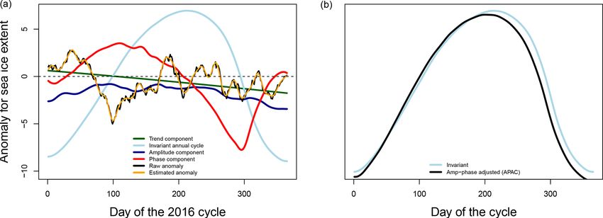
M. S. Handcock and M. N. Raphael: Modeling the annual cycle                                                                            2163

Figure 2. Comparison of annual cycle estimates: (a) a traditional and invariant cycle and (b) a traditional and amplitude- and phase-adjusted
cycle. The horizontal axis is the day of the cycle and the vertical axis is sea ice extent in millions of square kilometers.

Phase-adjusted annual cycle

Another component of the annual cycle that is important is               extent(t) = aP [phase(t)] + α(t),                               (7)
the phase. This is the timing of the maximum and minimum
extents. It is important because it determines the length of the         where phase(t) is the phase-adjusted day of the year for t
annual cycle and influences its shape. We enable the annual              (e.g., 164). It is a smooth function of time that tells us what
cycle to vary from year-to-year as a parameterized function              day of an invariant 365 d cycle the date t is. The function
of the phase of the annual cycle shape function, defining the            phase(t) is modeled here as follows:
phase-adjusted annual cycle, aP [s], as follows:

https://doi.org/10.5194/tc-14-2159-2020                                                         The Cryosphere, 14, 2159–2172, 2020
2164 M. S. Handcock and M. N. Raphael: Modeling the annual cycle
(APAC), aAP [s], as follows:
phase(t) = 365 extent(t) = aA [phase(t), min · extent(year(t)),
max · extent(year(t))] + α(t), (11)
t − min · extent · day(year(t))
× Beta
max · extent · day(year(t) + 1) ; β(year(t))
where aA and phase(t) are defined as in Eqs. (5) and (9). Note
that they will be different functions as they are now jointly
−min · extent · day(year(t))
specified. As before, aA [s] is modeled as a cyclic cubic spline
(8)
function of s chosen to minimize the penalized-square error:
min · extent · day(year(t)) ≤ t ≤ max · extent · day(year(t)),
(9) PSEλAPAC ,β (u) =
T
where max · extent · day(y) is the day of the year giving X extent(t) − min · extent(year(t))
the maximum extent for year y and min · extent · day(y)) is max · extent(year(t)) − min · extent(year(t))
t=T0
the day of the year giving the maximum extent for year y. 2
Here Beta(p; β), 0 ≤ p ≤ 1, is the cumulative distribution
− u[phase(t; β(year(t))]
function of a Beta(β) random variable parameterized by
β = (β1 > 0, β2 > 0) and β(y) is the parameter value spe- Z365
cific to year y.
+ λA u00 [s]2 ds λAPAC > 0, (12)
Here aP [s] is an invariant annual cycle for the extent (typ-
ically differing from aI [s]). It is defined in an analogous way 0
to the other invariant annual cycles as a cyclic cubic spline where λAPAC is a smoothing parameter. The minimization is
function of s chosen to minimize the penalized-square error: also over the parameters {β1 (y) > 0, β2 (y) > 0}2018
y=1978 . As
2 for the other annual cycles (invariant, amplitude-adjusted,
T
PSEλP ,β (u) =
X
extent(t) − u[phase(t; β(year(t))] phase-adjusted), λAPAC is chosen by generalized cross-
t=T0
validation.
Figure 2b compares the traditional annual cycle with the
Z365
recorded SIE for 2016 and the APAC produced by this model
+ λP u00 [s]2 ds (10) for the same time period. The APAC is a much better fit to the
0 recorded data and represents a large and significant improve-
λP > 0, β(year(t)) > 0, ment of 77.3 % in MSE (Table 1). Table 1 clearly demon-
strates the value of having multiple successive definitions of
where λP is a smoothing parameter, chosen to balance the the annual cycle when decomposing the variation in the daily
closeness of fit to the recorded values (the first term) with the annual cycle of SIE.
smoothness of u[s] (the second term). The minimization is The discussion above describes several different ways of
also over the parameters {β1 (y) > 0, β2 (y) > 0}2018y=1978 . defining the annual cycle of SIE. While an annual cycle ad-
The phase-adjusted annual cycle gives a different decom- justed for phase or amplitude only would not be the best esti-
position of the extent to the invariant annual cycle as it cap- mate for the data, differences between them and the optimal
tures variation due to phase variation. It allocates the compo- estimated annual cycle (i.e., APAC) could reveal sources of
nent of the variation in extent due to phase variation to the variability in the daily SIE.
annual cycle rather than the residual term, α(t).
Surprisingly, the adjustment for phase shows even more 3.2 Analyzing variation: volatility, daily rate of change,
improvement (63.9 %) in the MSE than that for the anomalies and trend
amplitude-adjusted annual cycle, indicating that the phase
contributes more to the variability of the annual cycle of SIE Estimating the annual cycle using our model allows us to
than the amplitude. Most studies of Antarctic sea ice vari- calculate statistics that reveal the underlying variability in
ability focus on the amplitude at maximum and minimum the daily SIE. Below we decompose the sea ice variation
extents, but this analysis indicates that the phase (the timing on the time dimension, moving up the temporal scale from
of these extrema) is at least as important a contributor to the the very short term (the instantaneous variation) to the day-
variability. to-day variation, followed by the interannual variation and
finally the multi-decadal variation, i.e., the trend.
Amplitude- and phase-adjusted annual cycle The recorded sea ice extent will deviate from the true sea
ice extent. This may be due to some combination of weather,
Finally, we can combine the amplitude and phase adjustment artifacts of the satellite algorithm used for retrieval, and the
ideas to define an annual cycle that jointly adjusts for both. electromagnetic spectrum across which the device or satellite
We define the amplitude- and phase-adjusted annual cycle is measuring, among other things. To represent this, we write
The Cryosphere, 14, 2159–2172, 2020 https://doi.org/10.5194/tc-14-2159-2020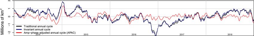
M. S. Handcock and M. N. Raphael: Modeling the annual cycle                                                                          2165

Table 1. Comparison of the various proposed annual cycles in terms of how well they explain the variation in daily SIE. Values are given as
percentages of mean-squared error and the root-mean-squared error (RMSE).

                                                                          Unexplained           Improvement
                                                                           variation in   in MSE compared to
                                Model                                     SIE (RMSE)           the Traditional
                                Overall mean (total variation)                    5.627                     –
                                Traditional annual cycle                          0.576                   0%
                                Invariant annual cycle                            0.482                28.7 %
                                Amplitude-adjusted                                0.382                55.2 %
                                Phase-adjusted                                    0.343                63.9 %
                                Amplitude- and phase-variation-adjusted           0.272                77.3 %

the recorded SIE, SIE(t), as follows:                                     on past volatilities is to better represent periods of high or
                                                                          low volatility. We also specify an autoregressive moving av-
SIE(t) = extent(t) + (t)                                                 erage (ARMA) model for α(t) (Box and Jenkins, 1976; Hipel
        = aA [phase(t), min · extent(year(t)),                            and McLeod, 1994) with (t) as the (time-dependent) error
              max · extent(year(t))] + α(t) + (t).              (13)     term. The model parameters were fit using maximum like-
                                                                          lihood. The Bayesian information criterion (BIC) was used
The recorded SIE on any given day is then the sum of a num-               to select the model order (Ghalanos, 2019). The model or-
ber of components of variation – the annual cycle for that                ders were p = 2 and q = 2 (i.e., GARCH(2,2)) and auto-
day, the yearly variation (anomaly) from the annual cycle and             regressive moving average, ARMA(1,1), for the anomaly
a residual term (*(t)). These are now discussed.                         model. All models were fit using the R package rugarch
                                                                          (Ghalanos, 2019).
3.2.1   Volatility of the recorded sea ice extent
                                                                             Figure 3 plots the average volatility in SIE, separating it
Here we introduce the term volatility to describe the instan-             into the two periods of time when different sensors were re-
taneous variation (or precision) in the recorded SIE as an                trieving the data. There is some indication that the volatil-
approximation for the extent. Such variation may be due to                ity is larger in the data recorded by the NIMBUS-7 Scan-
ephemeral effects like those mentioned above.                             ning Multi-channel Microwave Radiometer (SMMR) sen-
   Normally the standard deviation of the residual, (t) in               sor (orange) than by the Defense Meteorological Satellite
Eq. (13), is represented as a constant over time. Here, how-              Program (DMSP) (black), especially at times of maximum
ever, we allow it to vary, explicitly representing it as a time-          SIE. This could be an effect of the sensor resolution (sen-
varying term or component. The volatility is therefore de-                sor footprint), which is actually smaller (higher resolution) in
fined as the time series formed by the standard deviation of              NIMBUS-7. These estimates adjust for the every-other-day
(t), t = T0 , . . ., T . It is a quantification of ephemeral effects.    sampling of the NIMBUS-7 sensor. Were this not adjusted
Effectively it shows the size and timing of the variability               for, the NIMBUS-7 values would be substantially higher than
associated with factors like instrument error or noise in the             the DMSP. That said, there are some important similarities.
recorded SIE.                                                             Volatility is least at SIE minimum, larger at SIE maximum
   To model the volatility, we specify a generalized au-                  and largest late in the cycle when the ice is experiencing its
toregressive conditional heteroskedasticity (GARCH) model                 largest rate of retreat. This latter characteristic is discussed
(Bollerslev, 1986) for the residual (t). The residual is split           below. The values from the DMSP era show that the volatil-
into a time-dependent standard deviation σ (t) representing               ity ranges approximately from 40 to 50 K km2 . These are rel-
the volatility and a series z(t) ∼ N (0, 1):                              atively small values compared to the total SIE but are quite
                                                                          large compared to the typical grid cell size. The fact that the
(t) = σ (t)z(t).                                                         volatility is not constant over the cycle may be exploited to
                                                                          get a better understanding of contributors to overall variabil-
Explicitly, the (squared) volatility is modeled as a weighted
                                                                          ity in SIE.
average of the past anomalies and (squared) volatilities:
                p
                X                     q
                                      X                                   3.2.2   Daily rate of change
σ 2 (t) = ω +         ηi (t − i) +         ψi σ 2 (t − i),
                i=1                   i=1
                                                                          It is useful to know the daily rate of change of SIE because
where the parameters ηi and φi represent dependency on the                it gives insight into the daily timing of growth (advance) and
past residuals and volatilities, while the parameter ω repre-             melt (retreat) of the sea ice. It is also an expression of the
sents a trend in volatility. The purpose of the dependency                phase of the annual cycle. Contemporary trends in Antarc-

https://doi.org/10.5194/tc-14-2159-2020                                                        The Cryosphere, 14, 2159–2172, 2020
2166 M. S. Handcock and M. N. Raphael: Modeling the annual cycle Figure 3. Volatility of the recorded SIE for the NIMBUS-7 era (26 October 1978 to 20 August 1987) and the DMSP era (21 August 1987 to 2018). It is averaged over each day of the cycle in these eras. The units are given in millions of square kilometers. The purple curve is the day-to-day change in SIE from Fig. 4 tic sea ice are shown to be linked to the changes in the tim- The SIE minimum (day 0, Julian day 46) is coincident ing (phase) of advance and retreat (e.g., Stammerjohn et al., with the minimum growth rate. The ice advances, reaching 2008). Note that the annual cycles have been defined as con- the maximum growth rate by day 81 and maintaining this tinuous in day. Hence, we can quantify the rate of change of maximum growth rate for approximately 40 d before slow- total Antarctic SIE by the derivative of an annual cycle shape ing to a minimum growth rate by day 225 (late September) function, a[s]. The precise definition of the rate of change of the cycle. Sea ice retreat begins at approximately day 225 differs in the choice of annual cycle that is used. As an exam- and occurs quite rapidly compared to the advance, reaching ple, the rate of change for both the traditional and invariant a maximum rate at day 308 (late December) before slow- annual cycles is plotted in Fig. 4, which shows the day-to- ing to a stop at day 365 (Julian day 46 or mid-February). day changes in the SIE over the 365 d cycle. As might be The rates of advance and retreat of the ice are not constant expected, the overall pattern of the traditional (orange line) over the annual cycle. The maximum rate of retreat of the and invariant annual cycles (black line) are quite similar to ice is more than twice the maximum rate of advance. Fig- each other. Both cycles show that the rates of growth and ure 4 illustrates and more precisely defines a key characteris- melt are variable over the cycle. However, compared to that tic of the Antarctic annual cycle, i.e., its asymmetry. The ice of the invariant cycle, the day-to-day change in the traditional grows (advances) steadily over a much longer period than it annual cycle is quite variable, making it difficult, if not im- decays (retreats). It has been suggested that this asymmetry possible, to make precise statements about the timing of ice in the annual cycle is a result of the influence of the semi- growth and decay. For example, around day 200 of the cycle, annual oscillation (SAO) of the Antarctic circumpolar trough there is a reduction in the variability of the traditional annual (Enomoto and Ohmura, 1990; Watkins and Simmonds, 1999) cycle. This pause might be due to some idiosyncrasy in the and an open-water (ice)–albedo feedback, with the latter be- data or it might be related to the relative stability of the ice ing the main driver for the rapid retreat of sea ice (Ohshima extent in the region of the SIE maximum. The smooth mono- and Nihashi, 2005). Ice budget analysis studies (Holland and tonic day-to-day change of the invariant annual cycle shows Kwok, 2012; Holland, 2014; Holland and Kimura, 2016) in- that the day-to-day change is very close to zero, indicating dicate that surface winds are also important in the advance that the latter reason is more likely. Therefore, the following and retreat of the ice as they drive advection of ice and diver- comments are based on the day-to-day change in the invari- gence within the pack. Recent modeling studies (Kusahara ant annual cycle. et al., 2019) suggest that ice advance is due chiefly to thermo- The Cryosphere, 14, 2159–2172, 2020 https://doi.org/10.5194/tc-14-2159-2020
M. S. Handcock and M. N. Raphael: Modeling the annual cycle                                                                       2167

dynamic processes (except in the Ross Sea) while ice retreat           We estimate the true anomaly by using Eq. (13), rewriting
is largely wind driven (or dynamic). Our study provides more        it as follows:
precise information on the timing of advance and retreat and
                                                                                            ˆ
                                                                    α̂(t) = SIE(t) − âA [phase(t), min · extent(year(t)),
on the length of the two major stages of the ice cycle (ice
growth: 225 d; ice retreat: 140 d) than can be obtained from                                   max · extent(year(t))] − ˆ (t).   (14)
monthly averaged data. This is significant because much of
                                                                    We use the estimate of the APAC and compute ˆ (t) from the
the variation in contemporary Antarctic SIE has been occur-
                                                                    GARCH model for the residual (t) from Sect. 3.2.1. The
ring at sub-monthly scales.
                                                                    estimated anomaly is quite close to the recorded anomaly as
   Taken together, the daily rate of change and the volatil-
                                                                    ˆ (t) is small in magnitude (see Figs. 3 and 7).
ity (Figs. 3 and 4) show, (1) The timing of lowest volatility
                                                                        Figure 5 plots three types of anomalies: the raw anomaly
may be related to the fact that there is relatively little ice at
                                                                    from the traditional annual cycle and the estimated anomalies
minimum; (2) During the period when ice is advancing most
                                                                    from the invariant and APAC. These show the last 5 years
swiftly, the volatility is low, responding to constant large-
                                                                    of the 42 years of satellite-observed data, 2014–2018. The
scale forcing; (3) During the period of slowing growth and
                                                                    anomalies of the three annual cycles are similar in sign; how-
maximum extent, volatility is high, perhaps due to the more
                                                                    ever, those for the APAC tend to be smaller. The similar-
frequent occurrence of storms during winter (Simmonds and
                                                                    ity in sign is expected, and the smaller size of the APAC
Keay, 2000) causing fluctuations at the sea ice edge rather
                                                                    anomalies arises because the APAC is a much better fit to the
than within the pack where the sea ice concentration is at or
                                                                    recorded data. The anomalies for the traditional and invariant
close to 100 %. This effect of the storms may be magnified
                                                                    annual cycles are not significantly different from each other
because at the ice maximum, the perimeter of the ice cover
                                                                    in size. This is expected given the small difference between
is also at or near its maximum, potentially allowing more ice
                                                                    the two shown in Fig. 2. We can clearly see the large negative
area to be affected; (4) Volatility begins to decrease as the
                                                                    anomaly in SIE at the end of 2016. The negative anomaly
sea ice retreats; but (5) increases to its maximum value when
                                                                    is larger in the traditional and invariant annual cycles than
the rate of retreat is largest. The late peak in volatility may
                                                                    in the APAC, demonstrating that the APAC is a better fit to
be due to the dynamic nature of the retreat. Anecdotally, the
                                                                    the recorded SIE; therefore, the anomaly is expected to be
sea ice extent anomalies of note tend to occur during the sea
                                                                    smaller.
ice maximum and the period immediately following (Turner
et al., 2017; Schlosser et al., 2018). The statistics examined      3.2.4     Trend
here are suggesting that these anomalies are probably asso-
ciated more strongly with dynamic forcing than thermody-            The trends in SIE for both the Arctic and Antarctic have been
namic.                                                              the subject of much study. Most studies assume a linear trend
                                                                    and employ a linear model of the monthly data to estimate
3.2.3   Anomalies                                                   those trends (e.g., Parkinson and Cavalieri, 2012). Instead,
                                                                    we remove this assumption of linearity and model the trend
The detection and analysis of anomalies (deviations from the
                                                                    in the daily data as a thin plate regression spline function of
annual cycle) is essential to the understanding of contribu-
                                                                    time (Wood, 2003). We added a term to our model for the
tors to variability. Here we discuss three different but related
                                                                    SIE representing this curvilinear trend and jointly estimate it
types of anomalies. First there is the true anomaly, repre-
                                                                    by minimizing the PSE (penalized-square error):
sented by α(t) in Eqs. (1), (11) and (13). This is the differ-
ence between the true SIE and the annual cycle, however it          PSEλI ,λtrend (a, trend) =
is defined. The true anomaly is the preferred anomaly but
                                                                    T                                               Z365
is unobtainable because of imprecision in measuring and re-         X
                                                                                                                   2
trieving the sea ice data. Second there is the raw anomaly,                {extent(t) − trend(t) − a[doy(t))]} + λI     a 00 [s]2 ds
                                                                    t=T0
i.e., the difference between the observed (recorded) SIE and                                                              0
the annual cycle. Here we focus on a statistical estimate of                   ZT
the true anomaly, α(t), which we denote as α̂(t). The esti-         + λtrend        trend00 (t)2 dt                               (15)
mate is preferable to the raw anomaly as it adjusts for the
                                                                               T0
volatility and should be closer to the true anomaly than the
raw anomaly.                                                        λI > 0, λtrend > 0,
                                                                    where trend00 (t) is the second derivative of trend(t) at time
                                                                    t and λtrend is a smoothing parameter specific to the trend
                                                                    and is chosen to balance the closeness of fit to the recorded
                                                                    values using generalized cross-validation (Wood, 2004). The
                                                                    last term also captures the beginning and end time smooth-
                                                                    ing.

https://doi.org/10.5194/tc-14-2159-2020                                                        The Cryosphere, 14, 2159–2172, 2020
2168 M. S. Handcock and M. N. Raphael: Modeling the annual cycle
Figure 4. Day-to-day change in the annual cycle of sea ice extent for the traditional (orange) and invariant (black) annual cycles. The
horizontal axis is the day of the cycle, and the vertical axis is change in sea ice extent in millions of square kilometers.
Figure 5. Comparison of anomalies from three annual cycle estimates for 2014–2018: the raw anomaly from the traditional annual cycle
(black), the estimated anomaly from the invariant annual cycle (blue), and the estimated anomalies from the amplitude- and phase-adjusted
annual cycle (red). The vertical axis is the anomaly in millions of square kilometers.
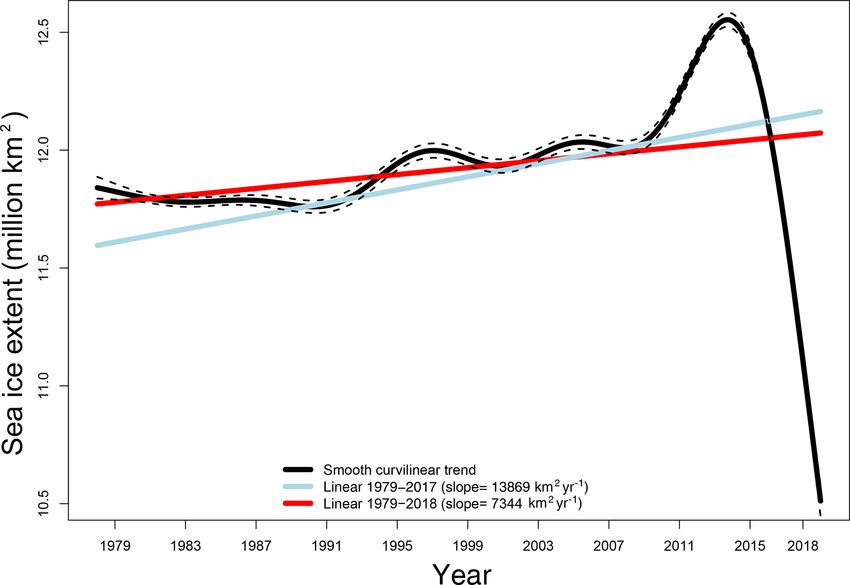
The curvilinear trend in SIE for 1979–2015 and 1979– nonlinearity of the daily SIE trend in this analysis is consis-
2018 derived using this method is illustrated in Fig. 6 along tent with that discussed by Simpkins et al. (2013) in their
with the linear estimates of the trend. The latter assumes the analysis of changes in the magnitudes of the sea ice trends
same model as Eq. (15) except it constrains trend(t) to be lin- in the Ross and Bellingshausen Seas. We note also that use
ear. While there is a small positive linear trend, as has been of the daily data adjusted for amplitude and phase potentially
reported in the literature (e.g., Parkinson and Cavalieri, 2012; allows a better estimate of the trend than monthly averaged
Turner et al., 2015a), Fig. 6 shows that there is strong non- values.
linearity in the trend. There are strong decadal differences. Even within the context of nonlinearity, the anomalously
For example, in the 1980s the trend was largely negative, low SIE represents a dramatic negative adjustment to Antarc-
while from 1990 to the mid-2000s there were a number of tic SIE (Schlosser et al., 2018; Parkinson, 2019), prompting
short-term fluctuations with opposing signs. It seems clear questions about whether or not this represents a change in
from Fig. 6 that the reported positive trend in total Antarc- state instead of a fluctuation due to natural variability. The
tic SIE is due largely to the positive trend that began at the current length of record does not allow much more than spec-
end of the first decade of the 21st century and continued un- ulation. However, we can decompose the annual cycle of
til 2016. The anomalously low SIE experienced since 2016 2016 into the various components of variation that we have
had the effect of reducing the slope of the linear trend by al- identified in this paper. This is illustrated in Fig. 7. The daily
most 50 % from 13 860 to 6068 km2 yr−1 . If the trends were values of the components are plotted against the anomaly in
linear they would be statistically significantly positive. The SIE, showing how much they contributed to the SIE anomaly.
The Cryosphere, 14, 2159–2172, 2020 https://doi.org/10.5194/tc-14-2159-2020M. S. Handcock and M. N. Raphael: Modeling the annual cycle 2169 Figure 6. Three estimates of the trend in the recorded SIE represented in terms of the amount of SIE associated with the change. The blue line is the linear trend estimated for data from 1 January 1979 to 31 December 2017. The red line is the linear trend estimated for data from 1 January 1979 to 31 December 2018. The black line is the curvilinear trend estimated for data from 26 October 1978 to 31 December 2019. The dashed lines are the 95 % pointwise confidence bands for the smooth curvilinear trend. Figure 7. (a) Decomposition of the sea ice extent during 2016 into various components of its variation, including separate amplitude and phase components. (b) The invariant and amplitude-adjusted annual cycles for 2016. Day of cycle is on the horizontal axis: day 0 is Julian day 52. Anomalous SIE in millions of kilometers squared is on the vertical axis. The decomposition is sequential with the amplitude compo- the difference between the recorded SIE and the APAC (the nent extracted before the phase component. anomaly that includes the volatility) and its smoothed ver- The decomposition shows that the curvilinear trend sion, the estimated anomaly (orange), is small and did not (green) for 2016 is small and positive early in the cycle and make a consistent contribution to the anomaly in SIE over the becomes strongly negative later in the year, making a large year. Smoothing removed the “noise”, which might be due to contribution to the negative anomaly during this time of rapid instrumentation and leaving behind a truer variation between change, as identified in Fig. 6. The raw anomaly (black), the recorded SIE and the expected SIE (i.e the APAC). The https://doi.org/10.5194/tc-14-2159-2020 The Cryosphere, 14, 2159–2172, 2020
2170                                                          M. S. Handcock and M. N. Raphael: Modeling the annual cycle

amplitude (blue) made a small but consistently negative con-        portant given that much of the contemporary variability in
tribution to the anomalously low SIE in 2016. Interestingly,        Antarctic sea ice occurs at sub-monthly scales. Combination
the main contributor to the anomalous SIE was the phase.            of the information given by the volatility and daily rate of
That is, the phase contributed to a small positive anomaly          change suggests that the volatility is lowest when the sea ice
during the growth stage of the cycle (the growth was slightly       is at its minimum and highest during the time of the max-
ahead of phase) and a strongly negative anomaly during re-          imum rate of retreat. Given that the rapid rate of retreat of
treat, indicating that the timing of retreat of the ice was ear-    the ice has been associated with dynamic processes, this sug-
lier than normal and the ice retreated faster than normal. The      gests that the peak in volatility at the end of the cycle is due
sum of these components (including the invariant annual cy-         to ephemeral effects associated with dynamic forcing.
cle (pale blue) is the recorded SIE for 2016. The decomposi-           To look at the interannual timescale, we defined and es-
tion shows that the difference between the recorded SIE and         timated several different but related anomalies, i.e., mea-
the traditional and invariant cycles seen in Fig. 2a is mostly      sures of deviation from the annual cycle, that may be used
due to phase, as is also seen in Fig. 7b.                           to evaluate the contributions to Antarctic sea ice variabil-
                                                                    ity from sources (local, oceanic and atmospheric) other than
                                                                    the large-scale sources that control cyclical, amplitude and
4   Conclusions                                                     phase changes. These show that our proposed annual cycle,
                                                                    the APAC, is a better fit to the recorded SIE.
Variability in the annual cycle of Antarctic sea ice extent is         We established that the trend in daily total Antarctic SIE
dominated by the amplitude and phase of the cycle. In this          over time is strongly nonlinear and that the linear estimates
study, we examined the variability in the annual cycle of to-       are weak and dependent on a positive trend that began in
tal Antarctic sea ice extent (SIE) in detail at timescales rang-    2011 and ended in 2016. Interestingly, our decomposition of
ing from instantaneous to day-to-day, interannual, and multi-       the annual cycle of 2016 into the components of variation
decadal trends, thus offering a complete picture of the tem-        defined in this paper shows that the main contributor to the
poral variation in the sea ice. To facilitate this analysis, we     anomalous SIE was the phase. That is, the anomalously low
developed first a statistical and mathematical model of the         SIE was due mainly to the fact that the retreat began earlier
annual cycle in which the amplitude and phase, the two ma-          than normal and was faster than normal. The amplitude made
jor contributors to its variability, are allowed to vary. This is   a much smaller negative contribution that did not vary much
contrary to traditional methods that restrict the variation in      over the year.
amplitude and phase, thus limiting their contribution to the           We used the daily total Antarctic SIE in this analysis.
variability. We define a number of complementary annual cy-         However, sea ice variability around Antarctica is strongly re-
cles – the invariant, which is an optimally smoothed annual         gional, and the annual cycles of these regions are markedly
cycle with no adjustments for phase or amplitude, an annual         different from each other and are also changing. The model-
cycle that adjusted for phase only, another adjusted for am-        estimated annual cycles and the timescale decomposition
plitude only, and one that is adjusted for phase and amplitude      presented here will facilitate examination of the regional
(APAC). Each of these annual cycles represent clear concep-         variability of Antarctic sea ice. Finally, although our method
tual and statistical improvements over the traditional method       was developed on Antarctic SIE, this decomposition method-
of calculating the annual cycle, with the APAC showing the          ology is applicable to a wide range of climatic variables (e.g.,
most improvement. We propose the APAC as a substitute for           temperature, Arctic sea ice extent) that experience an annual
the traditional method. However, the differences between the        cycle.
other annual cycles and the APAC reveal sources of variabil-
ity in the daily SIE. For example, comparing the annual cy-
cles adjusted for phase only and amplitude only revealed that       Code and data availability. The data used to generate the sea ice
the phase contributes more to the variability in the annual         extent are freely available from the National Snow and Ice Data
cycle than the amplitude.                                           Center (NSIDC) (Peng et al., 2013; Meier et al., 2017). The R lan-
   The timescales into which the variability of SIE was de-         guage (R Core Team, 2019) software used to produce the analysis
                                                                    in this paper is available on an open-source repository on GitHub
composed allow useful interpretations of the factors that give
                                                                    (Handcock et al., 2020). All figures and numbers in this paper can
rise to the variability. Using the volatility defined and de-       be reproduced.
scribed here for the first time, we show how much of the
total SIE is due to transient effects (such as satellite effects
and algorithmic artifacts). We also show how those effects          Author contributions. MNR conceived the idea for this study.
vary over the annual cycle, and in the process we note that         MNR and MSH developed the statistical methodology and analyzed
there are differences in the volatility (and hence uncertainty)     the data equally. MSH wrote the software and process of the data.
that arise because of sensor type. The daily rate of change         Both authors assisted in writing and editing the manuscript.
in SIE allows a precise definition of the timing and rate of
advance and retreat of the sea ice, a quality that is very im-

The Cryosphere, 14, 2159–2172, 2020                                                     https://doi.org/10.5194/tc-14-2159-2020
M. S. Handcock and M. N. Raphael: Modeling the annual cycle 2171
Competing interests. The authors declare that they have no conflict Holland, P. and Kwok, R.: Wind-driven trends in
of interest. Antarctic sea-ice drift, Nat. Geosci., 5, 872–875,
https://doi.org/10.1038/ngeo1627, 2012.
Holland, P. R.: The seasonality of Antarctic sea
Acknowledgements. The authors wish to thank Will Hobbs and ice trends, Geophys. Res. Lett., 41, 4230–4237,
Laura Landrum for their insight. https://doi.org/10.1002/2014GL060172, 2014.
Holland, P. R. and Kimura, N.: Observed Concentration Budgets
of Arctic and Antarctic Sea Ice, J. Climate, 29, 5241–5249,
Financial support. This research has been supported by the Na- https://doi.org/10.1175/JCLI-D-16-0121.1, 2016.
tional Science Foundation, Office of Polar Programs (grant no. Kusahara, K., Williams, G., Massom, R., Reid, P., and Ha-
NSF-OPP-1745089). sumi, H.: Spatiotemporal dependence of Antarctic sea ice vari-
ability to dynamic and thermodynamic forcing: A coupled
ocean–sea ice model study, Clim. Dynam., 52, 3791–3807,
https://doi.org/10.1007/s00382-018-4348-3, 2019.
Review statement. This paper was edited by Ted Maksym and re-
Meehl, G. A., Arblaster, J. M., Chung, C. T. Y., Holland, M. M., Du-
viewed by Walter Meier and one anonymous referee.
Vivier, A., Thompson, L., Yang, D., and Bitz, C. M.: Sustained
ocean changes contributed to sudden Antarctic sea ice retreat in
late 2016, Nat Commun., 10, 14, https://doi.org/10.1038/s41467-
018-07865-9, 2019.
Meier, W. N., Fetterer, F., Savoie, M., Mallory, S., Duerr, R.,
References and Stroeve, J.: NOAA/NSIDC climate data record of pas-
sive microwave sea ice concentration, Version 3, NSIDC: Na-
Bollerslev, T.: Generalized autoregressive conditional tional Snow and Ice Data Center, Boulder, Colorado USA,
heteroskedasticity, J. Econometrics, 31, 307–327, https://doi.org/10.7265/N59P2ZTG, 2017.
https://doi.org/10.1016/0304-4076(86)90063-1, 1986. Ohshima, K. I. and Nihashi, S.: A simplified ice-ocean coupled
Box, G. E. P. and Jenkins, G. M.: Time Series Analysis : Forecasting model for the Antarctic ice melt season, J. Phys. Oceanogr., 35,
and Control, Holden-Day, San Francisco, rev. ed. edn., 1976. 188–201, https://doi.org/10.1175/JPO-2675.1, 2005.
Comiso, J.: Bootstrap sea ice concentrations from NIMBUS- Parkinson, C. L.: A 40-y record reveals gradual Antarctic sea ice
7 SMMR and DMSP SSM/I-SSMIS, Version 3, increases followed by decreases at rates far exceeding the rates
https://doi.org/10.5067/7Q8HCCWS4I0R, 2017. seen in the Arctic, P. Natl. Acad. Sci. USA, 116, 14414–14423,
Comiso, J. C. and Steffen, K.: Studies of Antarctic sea ice con- https://doi.org/10.1073/pnas.1906556116, 2019.
centrations from satellite data and their applications, J. Geophys. Parkinson, C. L. and Cavalieri, D. J.: Antarctic sea ice vari-
Res.-Oceans, 106, 31361–31285, 2001. ability and trends, 1979–2010, The Cryosphere, 6, 871–880,
Craven, P. and Wahba, G.: Smoothing noisy data with spline func- https://doi.org/10.5194/tc-6-871-2012, 2012.
tions: Estimating the correct degree of smoothing by the method Peng, G., Meier, W. N., Scott, D. J., and Savoie, M. H.: A long-term
of Generalized Cross-validation, Numer. Math., 31, 377–403, and reproducible passive microwave sea ice concentration data
https://doi.org/10.1007/BF01404567, 1978. record for climate studies and monitoring, Earth Syst. Sci. Data,
Enomoto, H. and Ohmura, A.: The influences of atmo- 5, 311–318, https://doi.org/10.5194/essd-5-311-2013, 2013.
spheric half-yearly cycle on the sea ice extent in the R Core Team: R: A language and environment for statistical
Antarctic, J. Geophys. Res.-Oceans, 95, 9497–9511, computing, R Foundation for Statistical Computing, Vienna,
https://doi.org/10.1029/JC095iC06p09497, 1990. Austria, available at: https://www.R-project.org/, last access:
Ghalanos, A.: rugarch: Univariate garch models, r package Ver- 12 June 2019.
sion 1.4-1., available at: https://CRAN.R-project.org/package= Schlosser, E., Haumann, F. A., and Raphael, M. N.: Atmospheric
rugarch, last access: 12 June 2019. influences on the anomalous 2016 Antarctic sea ice decay, The
Handcock, M. S., Raphael, M. N., and Fogt, R.: Tools for un- Cryosphere, 12, 1103–1119, https://doi.org/10.5194/tc-12-1103-
derstanding the variability of climatic variables that experi- 2018, 2018.
ence an annual cycle, GitHub, Los Angeles, CA, available Simmonds, I. and Keay, K.: Mean southern hemisphere extra-
at: https://github.com/RaphaelLab/SeaIceVariation, last access: tropical cyclone behavior in the 40-year NCEP-NCAR re-
21 June 2020. analysis, J. Climate, 13, 873–885, https://doi.org/10.1175/1520-
Hipel, K. W. and McLeod, A. I.: Time Series Modelling of Wa- 0442(2000)0132.0.CO;2, 2000.
ter Resources and Environmental Systems, Elsevier, Amsterdam, Simpkins, G. R., Ciasto, L. M., Thompson, D. W. J., and England,
New York, 1994. M. H.: Seasonal relationships between large-scale climate vari-
Hobbs, W. R., Bindoff, N. L., and Raphael, M. N.: New perspec- ability and Antarctic sea ice concentration, J. Climate, 25, 5451–
tives on observed and simulated Antarctic sea ice extent trends 5469, https://doi.org/10.1175/JCLI-D-11-00367.1, 2012.
using optimal fingerprinting techniques, J. Climate, 28, 1543– Simpkins, G. R., Ciasto, L. M., and England, M. H.: Ob-
1560, https://doi.org/10.1175/JCLI-D-14-00367.1, 2015. served variations in multidecadal Antarctic sea ice trends
Holland, M. M., Landrum, L., Raphael, M., and Stammer- during 1979–2012, Geophys. Res. Lett., 40, 3643–3648,
john, S.: Springtime winds drive Ross sea ice variability https://doi.org/10.1002/grl.50715, 2013.
and change in the following autumn, Nat Commun., 8, 731,
https://doi.org/10.1038/s41467-017-00820-0, 2017.
https://doi.org/10.5194/tc-14-2159-2020 The Cryosphere, 14, 2159–2172, 20202172 M. S. Handcock and M. N. Raphael: Modeling the annual cycle Stammerjohn, S. E., Martinson, D. G., Smith, R. C., Yuan, X., and Turner, J., Phillips, T., Marshall, G. J., Hosking, J. S., Pope, J. O., Rind, D.: Trends in Antarctic annual sea ice retreat and advance Bracegirdle, T. J., and Deb, P.: Unprecedented springtime retreat and their relation to El Niño–Southern Oscillation and South- of Antarctic sea ice in 2016, Geophys. Res. Lett., 44, 6868–6875, ern Annular Mode variability, J. Geophys. Res.-Oceans, 113, https://doi.org/10.1002/2017GL073656, 2017. C03S90, https://doi.org/10.1029/2007JC004269, 2008. Watkins, A. B. and Simmonds, I.: A late spring surge in the open Stuecker, M. F., Bitz, C. M., and Armour, K. C.: Conditions lead- water of the Antarctic sea ice pack, Geophys. Res. Lett., 26, ing to the unprecedented low Antarctic sea ice extent during the 1481–1484, https://doi.org/10.1029/1999GL900292, 1999. 2016 austral spring season, Geophys. Res. Lett., 44, 9008–9019, Wegman, E. J. and Wright, I. W.: J. Am. Stat. Assoc., 78, 351–365, https://doi.org/10.1002/2017GL074691, 2017. 1983. Turner, J., Hosking, J. S., Bracegirdle, T. J., Marshall, Wood, S. N.: Thin plate regression splines, J. R. Stat. Soc., 1, 95– G. J., and Phillips, T.: Recent changes in Antarctic sea 114, 2003. ice, Philos. T. R. Soc. Lond., 373, 20140163–20140163, Wood, S. N.: Stable and efficient multiple smoothing parameter es- https://doi.org/10.1098/rsta.2014.0163, 2015a. timation for generalized additive models, J. Am. Stat. Assoc., 99, Turner, J., Hosking, S., Bracegirdle, T., Marshall, G., and Phillips, 673–686, 2004. T.: Recent changes in Antarctic sea ice, Philos. T. R. Soc. A, 373, Wood, S. N.: Generalized Additive Models: An Introduction with R, 20140163, https://doi.org/10.1098/rsta.2014.0163, 2015b. 2nd edn., Chapman & Hall/CRC, Boca Raton, 2017. The Cryosphere, 14, 2159–2172, 2020 https://doi.org/10.5194/tc-14-2159-2020
You can also read