Measurements of the water balance components of a large green roof in the greater Paris area
←
→
Page content transcription
If your browser does not render page correctly, please read the page content below
Earth Syst. Sci. Data, 12, 1025–1035, 2020
https://doi.org/10.5194/essd-12-1025-2020
© Author(s) 2020. This work is distributed under
the Creative Commons Attribution 4.0 License.

            Measurements of the water balance components of a
                 large green roof in the greater Paris area
        Pierre-Antoine Versini1 , Filip Stanic1,2 , Auguste Gires1 , Daniel Schertzer1 , and Ioulia Tchiguirinskaia1
                            1 HM&Co,      École des Ponts ParisTech, Champs-sur-Marne, 77455, France
                             2 Navier,   École des Ponts ParisTech, Champs-sur-Marne, 77455, France
                          Correspondence: Pierre-Antoine Versini (pierre-antoine.versini@enpc.fr)

                                  Received: 3 October 2019 – Discussion started: 19 November 2019
                            Revised: 28 February 2020 – Accepted: 24 March 2020 – Published: 6 May 2020

       Abstract. The Blue Green Wave of Champs-sur-Marne (France) represents the largest green roof (1 ha) of the
       greater Paris area. The Hydrology, Meteorology and Complexity lab of École des Ponts ParisTech has chosen
       to convert this architectural building into a full-scale monitoring site devoted to studying the performance of
       green infrastructures in storm-water management. For this purpose, the relevant components of the water bal-
       ance during a rainfall event have been monitored: rainfall, water content in the substrate, and the discharge
       flowing out of the infrastructure. Data provided by adapted measurement sensors were collected during 78 d
       between February and May 2018. The related raw data and a Python program transforming them into hy-
       drological quantities and providing some preliminary elements of analysis have been made available. These
       measurements are useful to better understand the hydrological processes (infiltration and retention) conducting
       green roof performance and their spatial variability due to substrate heterogeneity. The data set is available here:
       https://doi.org/10.5281/zenodo.3687775 (Versini et al., 2019b).

1   Introduction                                                       By increasing the storage of water, green roofs contribute
                                                                    to reducing the rainwater reaching the storm-water manage-
                                                                    ment network. It is particularly relevant to comply with regu-
Considered to be part of Blue Green Solutions (BGS), green          lation rules that are generally adopted by local authorities in
roofs are recognized as multifunctional assets able to pro-         charge of storm-water management, usually divided in two
vide several ecosystem services (Francis and Jensen, 2017;          categories: flow-rate-based regulation and volume-based reg-
Oberndorfer et al., 2007) to face climate change and un-            ulations (Petrucci et al., 2013). As green roofs perform both
sustainable urbanization consequences (such as biodiversity         retention (ability to permanently hold back water by storing
conservation or thermal insulation). They appear to be par-         the water for subsequent removal by evapotranspiration) and
ticularly relevant in storm-water management as they have           detention (ability to temporarily hold back the water) (Jo-
the ability to store a more or less significant portion of pre-     hannessen et al., 2018), they can be used as relevant tools to
cipitation (Stovin et al., 2012; Versini et al., 2016). Indeed,     ensure both kinds of regulation.
at the building scale, green roofs contribute to (i) reducing          Indeed, for a green roof located in the greater Paris area
runoff volume at the annual scale and (ii) attenuating and de-      (characterized by a temperate climate), the water balance
laying the peak at the rainfall event scale. This performance       during a rainfall event can be reduced to three components
depends on the green roof properties (substrate depth, poros-       (see Eq. 1) as evapotranspiration can be neglected:
ity, or vegetation type), rainfall intensity, and antecedent soil
moisture conditions (Berndtsson, 2010). Considered to be            P = Q + 1S,                                                (1)
storm-water source control facilities, they can act to man-
age rainwater at a small scale (about 102 –103 m2 ) to solve or     where P is the precipitation, Q the discharge flowing out
prevent intermediate-scale (104 – 106 m2 ) storm-water issues.      of the structure, and 1S the variation in water stored in the

Published by Copernicus Publications.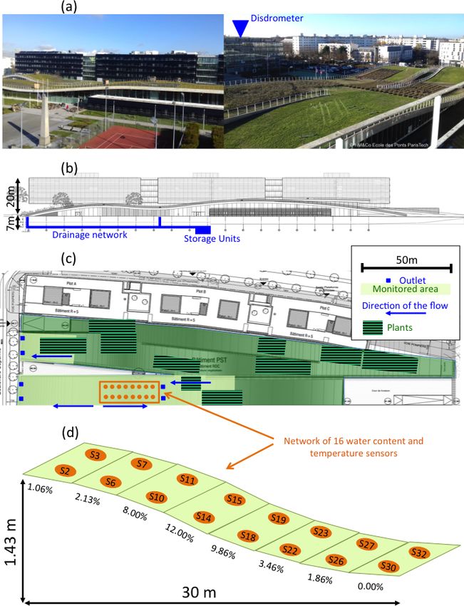
1026                                                                                    P.-A. Versini et al.: BGW water balance

substrate conducting both retention and detention properties.       consisting of a runoff chamber with an outlet weir and an
All quantities are expressed in cubic metres.                       ultrasonic sensor (to detect water level). The site was also
   Many experimental set-ups were implemented to moni-              equipped with a weather station measuring several meteoro-
tor, assess, and understand the hydrological behaviour of           logical variables (rainfall, wind speed, wind direction, rela-
green roofs (see Berndtsson, 2010, for a review). Most of           tive humidity, atmospheric temperature, etc.).
them were conducted on small green roof modules or plots               Although these works were focused on the hydrological
(Berretta et al., 2014; Getter et al., 2007; Li and Babcock,        behaviour of green roofs, few of them have actually mon-
2015; Locatelli et al., 2014; Loiola et al., 2019; Poë et al.,      itored the three components of the water balance. Rainfall
2015; Stovin et al., 2015; Wong and Jim, 2015; Zhang et             and discharge were generally considered to be sufficient to
al., 2015) characterized by an area ranging from 0.5 to 3 m2 .      assess its performance. Some additional studies can also be
These modular structures make possible the modification of          mentioned, but as they were focused on other topics (evap-
green roof configuration and study of the effects of substrate      otranspiration processes, Feng et al., 2018; or water quality,
(depth and nature), vegetation type, slope, or climate condi-       Buffam et al., 2016), only one component on the water bal-
tions on its performance. Some of them were also monitored          ance was assessed.
in controlled conditions (Ouldboukhitine et al., 2011; Poë et          The full-scale monitoring experiments mentioned above
al., 2015) to assess the respective impacts of temperature, ir-     also suffered from two limitations. First, they were still ded-
rigation, and light on green roof behaviour for instance.           icated to rather small green roof areas. As the hydrologi-
   In addition, few studies were conducted at full-scale green      cal performance of a green roof is influenced by the size
roofs. Indeed, such large structures were usually not planned       of the plot (water detention depends on water routing in the
for monitored during their construction and became hard to          structure for instance), larger infrastructure should be stud-
be monitored after. For instance, once built, electric connec-      ied. Second, very few measurements are performed (usually
tion is rarely compatible with the conservation of the roof         only one!) to assess water content on the whole vegetated
sealing. To the knowledge of the authors, only the following        surface. Indeed, green roof substrates – which are usually
works can be mentioned.                                             largely composed of mineral components – are very hetero-
   Palla et al. (2009a) studied an instrumented portion             geneous, causing variability in their infiltration and retention
(170 m2 ) of a green roof in Genoa (Italy) under the Mediter-       capacities. Therefore, large-scale monitoring set-ups able to
ranean climate. This pilot site was equipped to monitor the         capture this heterogeneity are required to better understand
different components of the water balance with a meteoro-           green roof hydrological behaviour and to study the space-
logical station for rainfall, several time domain reflectometry     time variability of the involved processes.
probes installed horizontally along a vertical profile for reten-      Based on these considerations, this paper aims to present
tion in the substrate, and triangular weir and tipping-bucket       and make available the water balance data collected on a
devices to follow the outflowing discharge.                         large green roof (called Blue Green Wave) located close to
   Hakimdavar et al. (2016) used the data collected on three        Paris (temperate climate) in order to study its hydrological
full-scale extensive green roofs in New York City (USA) to          behaviour and its ability to be used as a storm-water man-
validate a modelling approach based on the Soil Water Ap-           agement tool. The monitoring set-up has been specifically
portioning Method (SWAM). Under a humid continental cli-            tailored to take into account the space-time variability of the
mate, these monitored drainage areas ranged between 310             water balance components.
and 940 m2 . The three main components of the water bal-
ance were measured: rainfall with a weather station, water
                                                                    2     Materials and method
content with soil moisture and water content reflectometer
sensors, and discharge with a custom-designed weir placed           2.1    The Blue Green Wave
in the drain of the green roof.
   Fassman-Beck et al. (2013) assessed several green roofs in       The Blue Green Wave (BGW) is a large (1 ha) wavy-form
Auckland (New Zealand) under a subtropical climate. Their           vegetated roof located in front of École des Ponts ParisTech
areas ranged between 17 and 171 m2 . As the experimental            (ENPC, Champs-sur-Marne, France). For now it represents
set-up was focused on the rainfall–runoff relationship, only        the largest green roof of the greater Paris area. From its im-
these components were measured: rainfall with a tipping-            plementation in 2013, the BGW has been considered to be a
bucket rain gauge and discharge (deduced from water level)          demonstrative site oriented to Blue Green Solutions research
from a water pressure transducer and a custom-designed ori-         (Versini et al., 2018). This experimental set-up started dur-
fice restricted device.                                             ing the European Blue Green Dream (BGD) project (http:
   Cipolla et al. (2016) analysed runoff from a 60 m2 green         //bgd.org.uk/, last access: 22 April 2020, funded by Climate-
roof in Bologna (Italy) characterized by a humid temper-            KIC) that aimed to promote a change of paradigm for ef-
ate subcontinental climate. Continuous weather data and             ficient planning and management of new or retrofitted ur-
runoff were especially monitored for modelling develop-             ban developments by promoting the implementation of BGS
ment. Runoff was estimated by using an in-pipe flowmeter            (Maksimovic et al., 2013). Monitoring was anticipated and

Earth Syst. Sci. Data, 12, 1025–1035, 2020                                          www.earth-syst-sci-data.net/12/1025/2020/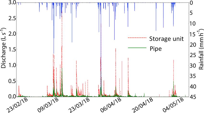
P.-A. Versini et al.: BGW water balance                                                                                          1027

Table 1. Physical properties of the BGW substrate.

                                                                                                        Saturated
                         Initial composition of the substrate   Porosity   Dry density     hydraulic conductivity
                         85 % of mineral matter and                40 %      1442 g l−1       8.11 × 10⁻⁶ m s−1
                         15 % of organic matter

the building was adapted for experimental purposes during              on a significant drained area collecting only the green roof
its construction. It was also supported by RadX@IdF, a re-             contribution (3511 m2 ). The implemented set-up is described
gional project that aimed at analysing the benefits of high-           in the following.
resolution rainfall measurement for urban storm-water man-
agement. Today the BGW is also part of the Fresnel multi-              2.2     Devices
scale observation and modelling platform created in the Co-
Innovation Lab at École des Ponts ParisTech. Fresnel aims              2.2.1    Rainfall measurement
to facilitate synergies between research and innovation, as
                                                                       Local rainfall has been analysed with the help of an optical
well as the pursuit of theoretical research, the development
                                                                       disdrometer: Campbell Scientific® PWS100. This device is
of a network of international collaborations, and various as-
                                                                       made of two receivers and a transmitter generating four laser
pects of data science (https://hmco.enpc.fr/portfolio-archive/
                                                                       sheets. By analysing the signals received from the light re-
fresnel-platform/, last access: 22 April 2020).
                                                                       fracted by each drop passing through the 40 cm2 sampling
   From a technical point of view, the BGW is covered by
                                                                       area, the drop size and velocity are estimated. A rain rate can
two types of vegetation: green grass that represents the large
                                                                       then be derived. Disdrometers are now considered to be a re-
majority of its area and a mix of perennial planting, grasses,
                                                                       liable rainfall measurement instrument (de Moraes Frasson
and iris bulbs (see Fig. 1). Vegetation is laid out on a sub-
                                                                       et al., 2011; Gires et al., 2016; Thurai et al., 2011). The de-
strate layer of about 200 mm depth (SOPRAFLOR I966),
                                                                       vice has been installed since September 2013 on the roof of
a filter layer made of synthetic fibre (SOPRATEX 650),
                                                                       the École des Ponts ParisTech building (see Fig. 1). This dis-
and a drainage layer made of expanded polystyrene (SO-
                                                                       drometer and its corresponding data have already been pre-
PRADRAIN). The vertical profile of the structure is pre-
                                                                       sented in detail in a previous data paper (Gires et al., 2018)
sented in Fig. 2. The substrate was initially composed of vol-
                                                                       that summarizes a measurement campaign that took place in
canic soil (around 85 %) completed by organic matter. It is
                                                                       January–February 2016. Here, the rainfall data provided by
worth noting that 50 % of the grains (in mass) are larger than
                                                                       this disdrometer and characterized by a time step of 30 s have
1.6 mm and 13 % of fine particles are smaller than 80 µm. The
                                                                       been used.
main physical properties of the substrate are synthesized in
Table 1 (see Stanic et al., 2019, for a detailed description in-
cluding grain size distribution, water retention, and hydraulic        2.2.2    Water content measurement
conductivity curves).
                                                                       Estimation of soil moisture represents a difficult challenge,
   From a hydrological point of view, the BGW is connected
                                                                       as it deals with a highly spatially and temporally variable pro-
to three storage units that collect rainwater coming from
                                                                       cess (Lakshmi et al., 2003), essentially due to soil type and
the roof (with pipes) but also from several impervious parts
                                                                       depth. Hence, suitable systems are required to properly as-
around the greened building. One of the storage units is pre-
                                                                       sess soil moisture. Today a large number of sensors based on
ceded by a smaller unit dedicated to irrigation. The water is
                                                                       different methods are available for this purpose (Jackson et
then routed to a large retention basin to collect excess vol-
                                                                       al., 2008). Among them, indirect methods based on electro-
umes of water during a rainfall event before being routed to
                                                                       magnetic (EM) principles have gained wide acceptance over
the storm-water management network. This retention basin
                                                                       the last decades. EM sensors have the advantage of deliver-
was designed (and oversized) because it was considered that
                                                                       ing fast, in situ, non-destructive, and reliable measurements
the green roof (representing 50 % of the total contributive
                                                                       with acceptable precision (Stacheder et al., 2009).
area) was totally impervious without any retention capac-
                                                                          Here the time domain reflectometry technique (TDR, also
ity. Until now in France, there have been neither rules nor
                                                                       known as capacitance) has been selected. It is an EM mois-
guidelines devoted to retention basin sizing that take into ac-
                                                                       ture measurement that determines an electrical property
count the retention properties of green areas. Therefore the
                                                                       called electrical conductivity or dielectric constant (ka ). It
follow-up on such infrastructure is particularly important to
                                                                       is based on the interaction of an EM field with the soil wa-
develop new guidelines or legislations. For this purpose, the
                                                                       ter by using capacitance and frequency domain technology
three components of the water balance have been monitored
                                                                       (Stacheder et al., 2009). The TDR sensor measures the prop-
on the BGW. This experiment has been particularly focused
                                                                       agation time of an EM pulse, generated by a pulse generator

www.earth-syst-sci-data.net/12/1025/2020/                                                 Earth Syst. Sci. Data, 12, 1025–1035, 2020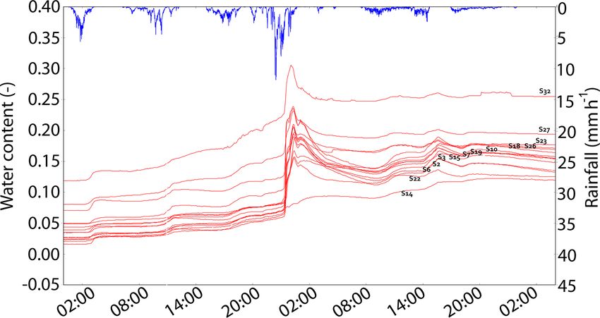
1028 P.-A. Versini et al.: BGW water balance
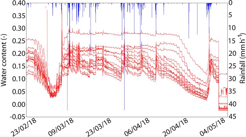
Figure 1. The Blue Green Wave monitoring site of ENPC: (a) pictures, (b) vertical representation and flow path lengths, (c) aerial rep-
resentation showing the monitored area, and (d) profile of the section where the water content sensors were implemented indicating the
slopes.
and containing a broad range of different measurement fre- Here ka is the bulk soil dielectric permittivity (unitless), L
quencies. The electrical pulse is applied to the waveguides the effective probe length (m), 1t the two-way travel time
(traditionally a pair of parallel metallic rods) inserted in the along the probe (s), and c the velocity of EM wave in free
soil. The incident EM travels across the length of the waveg- space (c = 2.298 × 10⁸ m s−1 )
uides and then is reflected back when it reaches the end of the It is then possible to estimate soil moisture content by
waveguides. The travel time required for the pulse to reach analysing the dielectric constant changes in the soil. The
the end of the waveguides and come back depends on the usual relationship between volumetric water content and di-
dielectric constant of the soil. electric constant is known as Topp’s equation (Topp et al.,
1980). It is adapted to a homogeneous conventional soil.
Note that this substrate can be considered coarse enough to
c · 1t
not clearly show the dielectric behaviour of a typical volcanic
ka = (2) media (see Palla et al., 2009b, for a similar assumption). For
2·L
Earth Syst. Sci. Data, 12, 1025–1035, 2020 www.earth-syst-sci-data.net/12/1025/2020/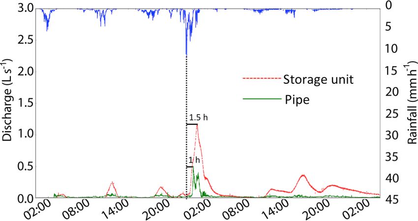
P.-A. Versini et al.: BGW water balance                                                                                      1029

                                                                   was responsible for many gaps in the time series due to in-
                                                                   terference between the different TDR sensors and the bases.
                                                                   To avoid this problem, only 16 TDR sensors were used, all
                                                                   of them connected to the same CWB100 base. For this same
                                                                   reason of possible interferences between the sensors, the time
                                                                   interval was enlarged to 4 min. Indeed, it is recommended to
                                                                   leave 15 s to ensure the connection of one sensor to the base.
                                                                   The final network aimed to capture the space-time variability
                                                                   of water content in a heterogeneous soil such as the BGW
                                                                   substrate. It was particularly adapted to assess the influence
                                                                   of the slope on infiltration and evapotranspiration processes.

                                                                   2.2.3   Discharge measurement
                                                                   Direct discharge measures are difficult to obtain in drainage
                                                                   pipes. For this reason, indirect measures using water level
                                                                   measurements are usually carried out. Here, water level in-
                                                                   side the pipes was measured by a UM18 ultrasonic sensor
                                                                   (SICK, 2018) produced by SICK® . This sensor has been es-
                                                                   pecially developed to perform non-contact distance measure-
                                                                   ment or detection of objects. The sensor head emits an ultra-
Figure 2. Vertical profile of the green wave structure.            sonic wave and receives the wave reflected back from the
                                                                   target. Ultrasonic sensors measure the distance to the target
                                                                   by measuring the time between the emission and reception.
this reason, it is assumed that the dielectric constant–water      Implemented with the face to the water surface, it also mea-
content relationship is not significantly different from the       sures the variation in the water level. The UM18 sensor is
Topp equation:                                                     characterized by a nominal range of 250 mm and an accuracy
                                                                   of 1 % for this measurement range. For the UM18 ultrasonic
θ = −5.3 × 10⁻² + 2.92 × 10⁻² ka − 5.5 × 10⁻⁴ ka2                  sensor, the dead zone is estimated to be 5 mm. As the sen-
  + 4.3 × 10⁻⁶ ka3 ,                                        (3)    sor has been placed on the top of the conduit, only very high
                                                                   values (higher than 240 mm) could be affected by this dead
where θ is the volumetric soil water content (m3 m−3 ).            zone. Since its implementation, water levels have never been
   As an alternative to Topp’s equation, an additional study       higher than 120 mm.
was conducted to assess this relationship in lab. Here, for           One UM18 sensor has been implemented inside a pipe
information, the calibration curve obtained with compaction        located in the garage in the building basement (see Fig. 1).
better representing the current condition is displayed. This       With a diameter of 300 mm, this pipe collects the water com-
compaction was artificially mimicked by applying vibrations        ing from a large part of the BGW (approximately 1143 m2 ).
(this causes the segregation of the material similar to what       A standard 4–20 mA current loop is used to monitor or re-
occurs in situ during a long period of time).                      motely control these analogue sensors. The current is then
                                                                   transformed in voltage by a resistance of 100. The result-
θ = −3.01 × 10⁻¹ + 1.13 × 10⁻¹ ka − 5.81 × 10⁻³ ka2                ing transmitted signal ranges from 400 to 2000 mV. In order
                                                                   to translate the electric signal in water level values, the fol-
  + 9.85 × 10⁻⁵ ka3                                         (4)
                                                                   lowing relationship has been applied:
Given that the dielectric data are provided, potential users are                        250
free to use Topp’s equation as in this paper, or another equa-     H0 = (U − 460) ×          .                                (5)
                                                                                        1600
tion.                                                              H0 is the water level in millimetres, U the measured voltage
   Consequently, a ubiquitous wireless TDR sensor network          in millivolts, 460 the offset, 250 the modified nominal range
has been implemented on the ENPC Blue Green Wave to                in millimetres, and 1600 the nominal range in millivolts.
measure both water content and temperature. For this pur-             The water level is then transformed into discharge by us-
pose 32 CWS665 wireless TDR sensors (produced by Camp-             ing the Manning–Strickler equation (Eq. 6). This formula is
bell Scientific® ) were initially installed. The data were col-    usually used to estimate the average velocity (and discharge)
lected by four CWB100 wireless bases, able to each store the       of water flowing in an open channel. It is commonly applied
data of eight sensors. Then the data were transferred to a CR6     in sewer design containing circular pipes.
data logger from Campbell Scientific® . The initial selected                               2    1
time step was 1 min. It appeared that this first configuration     Q0 = V × S = K × R 3 × i 2 × S                              (6)

www.earth-syst-sci-data.net/12/1025/2020/                                         Earth Syst. Sci. Data, 12, 1025–1035, 2020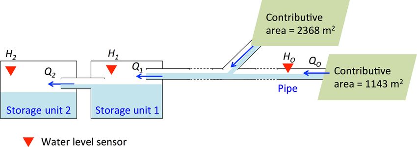
1030                                                                                    P.-A. Versini et al.: BGW water balance

Figure 3. Location of the water level sensors in the storm-water
management network.

Here V is the average water velocity (m s−1 ), K the friction
coefficient (unitless), S the wet surface (m2 ), R the hydraulic
radius (m), and i the pipe slope (m m−1 ), which is equal to       Figure 4. Relationship adjusted between the water level H1 and the
0.0074 here. R and S are directly linked to the water level.       downstream discharge Q2 .

     S
R=                                                          (7)       Finally, discharge data were recorded with a time step of
     P
                                                                   30 s for the sensor implemented in the conduit and 15 s for
    (θ − sin (θ)) × r 2
S=                                                          (8)    the one in the storage unit.
            2
P = r ×θ                                                    (9)
                                                                 2.3   Available output, data processing, and period of
                  r −H                                                   study
θ = 2 × arccos                                             (10)
                    r
                                                                   As already presented in detail in Gires et al. (2018), precipi-
K has been chosen to be 85. This value corresponds with a          tation data are collected in real time and stored through daily
cast iron material.                                                files. Here, these files for a 30 s time step rain rate have been
   Two additional UM18 sensors have been implemented in            gathered with the help of a Python script to create a long time
the two consecutive storage units (see Fig. 3) collecting the      series covering the whole period of study. Each line contains
rainwater drained by a large contributive area of 3511 m2 and      the time step expressed as YYYY-MM-DD HH:MM:SS and
including the previous monitored area. The first storage unit      the corresponding rainfall intensity (mm h−1 ) separated by a
is a rainwater tank (characterized by a floor area of 32.2 m2 )    comma.
devoted to irrigation. Filled most of the time, the excess wa-        Water content and water level data inside the pipe are col-
ter is routed by a pipe toward the second unit (floor area of      lected and stored every night on the HM&Co server in two
22.5 m2 ). A relationship similar to Eq. (5) between the volt-     different files. For this purpose, the Loggernet software pro-
age measurement and the water level has been adjusted for          duced by Campbell Scientific® has been used. It supports
both units:                                                        programming, communication, and data retrieval between
                                                                   data loggers and a PC. Concerning the water level file, each
                      20
Hi = (U − 0.38) ×         − dh.                            (11)    line corresponds to a time step for which the following infor-
                     1.62                                          mation is recorded (in each line, these values are separated
Here U is the measured voltage in volts, the nominal range is      by a comma):
20 cm, and dh (equal to 1.06 cm) corresponds to an additional
                                                                     – exact definition of the time step expressed as YYYY-
offset due to the elevation of the sensor
                                                                       MM-DD HH:MM:SS,
   By studying both water level variations, a relationship be-
tween the water level measured in the first unit (H1 ) and the       – item number,
outflow routing to the second unit Q2 (and related to H2 )
has been established (see Fig. 4). Finally, the total discharge      – voltage indicator to ensure the quality of the measure-
reaching the first unit and collecting the downstream rainfall         ment (it should be close to 12 V),
can be assessed by the following equation depending only on          – internal temperature of the data-logger box,
H1 :
                                                                     – unused data coming from a non-operational sensor,
             dH1                  dH1
Q1 = Q2 +        × A1 = f (H1 ) +     × A1,                (12)      – water level measured inside the pipe (U in Eq. 6, ex-
              dt                   dt
                                                                       pressed in millivolts),
where Q1 is the discharge reaching the first unit and Q2 the
second unit; A1 = 33.2 m2 is floor area of the first unit.           – unused data coming from a non-operational sensor,

Earth Syst. Sci. Data, 12, 1025–1035, 2020                                         www.earth-syst-sci-data.net/12/1025/2020/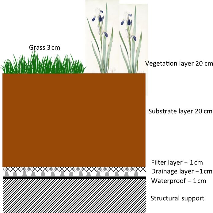
P.-A. Versini et al.: BGW water balance                                                                                      1031

    – unused data coming from a non-operational sensor.             for security reason. Nevertheless, during several months
                                                                    at the beginning of 2018, they were maintained on the
A similar format has been chosen for volumetric water con-          same section of the BGW (the one showed in Fig. 1).
tent data (note that names of the 16 volumetric water content       This time period corresponds to 78 d, from 19 February
(VWC) sensors are indicated in the header and are also re-          to 7 May 2018. After this period, the water content sen-
ported in Fig. 1):                                                  sors were moved to proceed to several evapotranspiration
    – exact definition of the time step expressed in YYYY-          measurement campaigns on the BGW (see Conclusion sec-
      MM-DD HH:MM:SS,                                               tion). This period has been selected to provide water bal-
                                                                    ance components measurements to potential users. This
    – item number,                                                  data set is available for download from the following web
                                                                    page: https://doi.org/10.5281/zenodo.3687775 (Versini et al.,
    – voltage indicator to ensure the quality of the measure-       2019b).
      ment (it should be close to 12 V),

    – internal temperature of the data-logger box,                  3.1   Presentation of the available data set

    – volumetric water content (expressed as ka ) for the 16        This data set presented in detail in the next section contains
      TDR sensors,                                                  the following files:

    – STT_B3: summary transfer time for basis, which is re-           – a rainfall file, 2018_0219-0507_Data_rainfall.csv;
      lated to the total time required for collecting information
                                                                      – a water content file, 2018_0219-0507_VWC.csv;
      from all the sensors that are collected to that base.
                                                                      – a file of the water level inside the pipe, 2018_0219-
Water level data inside the storage units have been collected
                                                                        0507_Data_discharge.csv;
by using the open-source Arduino Uno microcontroller board
that works in the offline regime. This Arduino system was             – a file of the water level in the storage, 2018_0219-
chosen because the storage unit was instrumented a few                  0507_Data_Arduino.csv;
months after the conduit and because the distance was too
long to make a connection between the storage unit and the            – a Python script to select the data, transform the raw data
existing data logger. Data are continuously stored on the 64            in physical measurements, and carry out some initial
MB memory card implemented in the board and copied man-                 analysis.
ually to the HM&Co server once per week. Data contain the
                                                                    In detail, the Python script is structured as follows.
following information (in each line, these values are sepa-
rated by a space):                                                    – Time period selection. This part could be changed to se-
                                                                        lect a study time period by choosing an initial and final
    – item number,
                                                                        date.
    – voltage values for the first storage unit – U 1 (in milli-
                                                                      – Data selection and transformation. The data corre-
      volts),
                                                                        sponding to this time period are selected in the differ-
    – voltage values for the second storage unit – U 2 (in mil-         ent files. Electric signals measured by the water level
      livolts),                                                         sensors are converted in water level (by using Eqs. 5
                                                                        and 11) and then in discharge by using the Manning–
    – exact definition of the time step expressed in YYYY-              Strickler equation (Eq. 6) for the pipe and Eq. (12) for
      MM-DD HH:MM:SS.                                                   the storage unit. In order to smooth the erratic 15 s sig-
                                                                        nal produced by storage unit measurements, the com-
By using Eq. (11) U 1 values are transformed into H 1 as a
                                                                        puted discharge data are averaged on a moving win-
part of post-processing. Note that U 2 data have been used
                                                                        dow, whose number of time steps can be modified. Di-
only for a short period of time after the implementation of
                                                                        electric constants measured by the 16 TDR sensors are
UM18 sensors, until Q2 = f (H 1) functionality has been ob-
                                                                        converted in water content by using the Topp equation
tained. After that they were no longer necessary.
                                                                        (Eq. 3).

3    Data availability                                                – Representation of the computed data. Several figures
                                                                        are plotted to illustrate the variation in the hydrological
Contrary to rainfall and discharge, which are measured                  components in time. The first one represents the cor-
continuously at the same locations, water content sensors               responding hydrographs for both discharges computed
can be moved from one location to another on the BGW.                   inside the pipe and in the storage unit. The second one
Moreover, they were rarely kept installed during the night              synthesizes the water content measured by the 16 TDR

www.earth-syst-sci-data.net/12/1025/2020/                                          Earth Syst. Sci. Data, 12, 1025–1035, 2020
1032 P.-A. Versini et al.: BGW water balance
sensors. In each figure, the precipitation is drawn on an
inverted y axis.
– Computation of runoff coefficients. Runoff coefficient
is the ratio between the total amount of precipitation
(computed by multiplying the rain depth by the corre-
sponding contributive area) and the total volume of wa-
ter flowing through the monitored pipe or the storage
unit. This value ranging from 0 % to 100 % illustrates
the capacity of the green roof to retain rainwater.
3.2 Presentation of the time series
Figure 5. Rainfall and computed discharges for the whole time pe-
During the available time period including half of winter and riod.
half of spring, it rained a total amount of 123.1 mm (see
Fig. 5). The rainfall file has no missing value, and six rain-
fall events can be defined. They correspond to periods with
cumulative rainfall depths greater than 5 mm (separated by a
dry period of at least 6 h) that caused discharge in both the
pipe and storage unit: 7 March (9 mm), 11 March (9.7 mm),
17 March (7.5 mm), 27 and 28 March (13.9 mm), 9 April
(9.6 mm), and 29 and 30 April (23.5 mm). These events are
obviously not representative of the full range of precipitation
events in the area. Nevertheless, it has to be mentioned that
since the BGW was monitored (2017), intense rainfall has
never caused any flooding on the surface or pipe filling (the
higher water level measured was about 12 cm).
Concerning the 16 VWC sensors, 5.6 % of the time steps Figure 6. Rainfall and volumetric water content (m3 m−3 ) for 16
are considered to be missing data. This is essentially due to TDR sensors.
two particular sensors that were out of service from 16 March
to the end of the study time period. The 16 sensors follow
the same dynamic, responding to the several rainfall events vegetation. It should be returned to the atmosphere by evapo-
(see Fig. 6). Water content measurements decrease simulta- transpiration. As already mentioned, Topp’s equation (Eq. 3)
neously during two long dry periods, at the end of February used to convert the dielectric constant to water content could
and from mid-April to the beginning of May. The sensors not be adapted to the specific substrate used for the BGW. For
show a significant spatial variability in terms of absolute val- this reason, the dielectric constant data are provided, leaving
ues. These differences illustrate the heterogeneousness of the the reader free to use another relationship to convert these
substrate profiles in terms of hydrological behaviour. This is data into water content.
due to the granular composition of the substrate but also to
the wavy form of the BGW. Indeed, the lowest values tend 3.3 Illustration with a particular event
to refer to the upstream sensors, whereas the highest values
tend to refer to the downstream ones. Note that the grain size The 29 and 30 April rainfall event is presented in details in
distribution time evolution is difficult to assess. Only the loss this section. It corresponds to the most intense event with
of some small particles has been noticed in the conduits. a total cumulative rainfall depth of 23.5 mm. Figure 7 shows
Discharge data are almost complete. Only one measure- the corresponding hydrograph from which the delay between
ment is missing in the pipe and 0.2 % of the total number rainfall and discharge peaks can be deduced. It reaches 1 h for
of time steps for the storage unit. These missing data corre- the first contributive area (drained to the pipe) and 1.5 h for
spond to the short periods during which the manual collec- the second one (drained to the storage unit).
tion of the data was carried out. Note that in order to avoid Regarding the question of coherency with previous studies
the loss of relevant data, this collection was done during a (Palla et al., 2009b, for instance), the water content differ-
dry period. Over this time period of 78 d, the runoff coef- ence was computed with Topp’s equation. The water stored
ficient computed for both pipe and storage unit is equal to in the substrate during this event was assessed according to
70.6 % and 71.1 % respectively. These close values demon- the difference between initial and final values. For the 16 sen-
strate the suitability of the monitored set-up. The missing wa- sors, this value ranges between 9.8 % and 13.7 %. This corre-
ter corresponds to the water retained by the substrate and the sponds to a water depth of between 19.6 and 27.2 mm and a
Earth Syst. Sci. Data, 12, 1025–1035, 2020 www.earth-syst-sci-data.net/12/1025/2020/P.-A. Versini et al.: BGW water balance 1033
and validate some appropriate modelling approaches (Stovin
et al., 2013; Versini et al., 2016).
This data set is available for download
free of charge from the following web page:
https://doi.org/10.5281/zenodo.3687775 (Versini et al.,
2019b).
It is provided by the Hydrology, Meteorology, and Com-
plexity laboratory of École des Ponts ParisTech (HM&Co-
ENPC). The following references should be cited for every
use of the data: Versini et al. (2019a, this paper).
Research focused on the assessment of ecosystem services
Figure 7. Rainfall and computed discharges for the 29–
provided by Blue Green Solutions is continuing at HM&Co-
30 April 2018 event. ENPC, and particularly on the BGW. The monitoring set-up
has been recently extended to the energy balance component
measurement (radiation balance, conduction, sensitive and
latent heat flux) and particularly to the evapotranspiration
flux. Such data will be particularly useful to study the ability
of Blue Green Solutions to mitigate urban heat islands (but
also to assess their retention potential during dry periods).
The French ANR EVNATURB project (https://hmco.enpc.fr/
portfolio-archive/evnaturb/, last access: 22 April 2020) that
aims to develop a platform to assess some of the ecosys-
tem services (i.e. storm-water management, cooling effect,
or biodiversity conservation) provided by BGS is now pursu-
ing this work of monitoring (Versini et al., 2017).
Figure 8. Rainfall and volumetric water content (m3 m−3 ) for 16
TDR sensors for the 29–30 April 2018 event (sensor references are Author contributions. P-AV supervised the study and reviewed
indicated by an increasing value at the end of the event). and wrote a large part of the manuscript; FS and AG worked on the
implementation of some of the presented sensors and the collection
of the data and participated in the review of the paper; DS and IT
storage capacity between 83 % and higher than 100 % of the collaborated on the study supervision and the review process.
rainfall (note that a range of between 20.6 and 30.0 mm is ob-
tained with the lab relationship presented in Eq. 4). It is clear
the larger values are overestimated but the order of mag- Competing interests. The authors declare that they have no con-
nitude is consistent with the computed runoff coefficients: flict of interest.
15 % for the surface drained to the pipe and 22 % for the sur-
face drained to the storage unit. This result illustrates the re-
tention and detention properties of the green roof. It has to be Acknowledgements. This work was initiated during the Climate-
KIC-funded Blue Green Dream project (http://bgd.org.uk/, last ac-
recalled that these impacts differ from one event to another
cess: 22 April 2020). It has also been supported by the Aca-
depending on the precipitation and the initial conditions. demic Chair “Hydrology for Resilient Cities”, a partnership be-
tween École des Ponts ParisTech and the Veolia group, and the ANR
4 Conclusions EVNATURB project dealing with the evaluation of ecosystem per-
formance for renaturing urban environments.
This paper presents the data collected by several devices de-
voted to the assessment of the water balance of a particular
green roof located close to Paris. The data set made avail- Financial support. This research has been supported by the
able for research purposes contains three types of data, repre- Climate-KIC, the Academic Chair “Hydrology for Resilient Cities”,
and the French Agence Nationale de la Recherche (ANR-17-CE22-
senting the relevant components of the water balance during
0002-01).
a rainfall event: rainfall, water content in the substrate, and
the discharge flowing out of the infrastructure. These data
were collected during 78 d between February and May 2018.
Review statement. This paper was edited by David Carlson and
These measurements are useful to study the capacity of such reviewed by two anonymous referees.
vegetated structures to store rainwater and act as a storm-
water management tool. They could also be useful to develop
www.earth-syst-sci-data.net/12/1025/2020/ Earth Syst. Sci. Data, 12, 1025–1035, 20201034 P.-A. Versini et al.: BGW water balance
References field experiments, Hydrol. Process., 17, 3041–3057,
https://doi.org/10.1002/hyp.1275, 2003.
Li, Y. and Babcock, R. W.: Modeling Hydrologic Performance
Berndtsson, J. C.: Green roof performance towards management of of a Green Roof System with HYDRUS-2D, J. Environ.
runoff water quantity and quality: A review, Ecol. Eng., 36, 351– Eng., 141, 4015036, https://doi.org/10.1061/(ASCE)EE.1943-
360, https://doi.org/10.1016/j.ecoleng.2009.12.014, 2010. 7870.0000976, 2015.
Berretta, C., Poë, S., and Stovin, V.: Moisture content behaviour in Locatelli, L., Mark, O., Mikkelsen, P. S., Arnbjerg-Nielsen,
extensive green roofs during dry periods: The influence of veg- K., Bergen Jensen, M., and Binning, P. J.: Mod-
etation and substrate characteristics, J. Hydrol., 511, 374–386, elling of green roof hydrological performance for ur-
https://doi.org/10.1016/j.jhydrol.2014.01.036, 2014. ban drainage applications, J. Hydrol., 519, 3237–3248,
Buffam, I., Mitchell, M. E., and Durtsche, R. D.: En- https://doi.org/10.1016/j.jhydrol.2014.10.030, 2014.
vironmental drivers of seasonal variation in green Loiola, C., Mary, W., and Pimentel da Silva, L.: Hydrological per-
roof runoff water quality, Ecol. Eng., 91, 506–514, formance of modular-tray green roof systems for increasing the
https://doi.org/10.1016/j.ecoleng.2016.02.044, 2016. resilience of mega-cities to climate change, J. Hydrol., 573,
Cipolla, S. S., Maglionico, M., and Stojkov, I.: A long- 1057–1066, https://doi.org/10.1016/j.jhydrol.2018.01.004, 2019.
term hydrological modelling of an extensive green Maksimovic, C., Stankovic, S., Liu, X., and Lalic, M.: Blue green
roof by means of SWMM, Ecol. Eng., 95, 876–887, dream project’s solution for urban areas in the future, Inter-
https://doi.org/10.1016/j.ecoleng.2016.07.009, 2016. national science conference reporting for sustainability, Becici,
Fassman-Beck, E., Voyde, E., Simcock, R., and Hong, Montenegro, 7–10 May 2013, 49–54, 2013.
Y. S.: 4 Living roofs in 3 locations: Does configura- Oberndorfer, E., Lundholm, J., Bass, B., Coffman, R. R., Doshi,
tion affect runoff mitigation?, J. Hydrol., 490, 11–20, H., Dunnett, N., Gaffin, S., Köhler, M., Liu, K. K. Y., and
https://doi.org/10.1016/j.jhydrol.2013.03.004, 2013. Rowe, B.: Green Roofs as Urban Ecosystems: Ecological
Feng, Y., Burian, S., and Pardyjak, E.: Observation and Es- Structures, Functions, and Services, BioScience, 57, 823–833,
timation of Evapotranspiration from an Irrigated Green https://doi.org/10.1641/B571005, 2007.
Roof in a Rain-Scarce Environment, Water, 10, 262, Ouldboukhitine, S.-E., Belarbi, R., Jaffal, I., and Trabelsi, A.:
https://doi.org/10.3390/w10030262, 2018. Assessment of green roof thermal behavior: A coupled heat
Francis, L. F. M. and Jensen, M. B.: Benefits of green and mass transfer model, Build. Environ, 46, 2624–2631,
roofs: A systematic review of the evidence for three https://doi.org/10.1016/j.buildenv.2011.06.021, 2011.
ecosystem services, Urban For. Urban Green, 28, 167–176, Palla, A., Gnecco, I., and Lanza, L. G.: Unsaturated 2D
https://doi.org/10.1016/j.ufug.2017.10.015, 2017. modelling of subsurface water flow in the coarse-grained
de Moraes Frasson, R. P., da Cunha, L. K., and Kra- porous matrix of a green roof, J. Hydrol., 379, 193–204,
jewski, W. F.: Assessment of the Thies optical dis- https://doi.org/10.1016/j.jhydrol.2009.10.008, 2009a.
drometer performance, Atmos. Res., 101, 237–255, Palla, A., Gnecco, I., and Lanza, L. G.: Unsaturated 2D
https://doi.org/10.1016/j.atmosres.2011.02.014, 2011. modelling of subsurface water flow in the coarse-grained
Getter, K. L., Rowe, D. B., and Andresen, J. A.: porous matrix of a green roof, J. Hydrol., 379, 193–204,
Quantifying the effect of slope on extensive green https://doi.org/10.1016/j.jhydrol.2009.10.008, 2009b.
roof stormwater retention, Ecol. Eng. 31, 225–231, Petrucci, G., Rioust, E., Deroubaix, J.-F., and Tassin,
https://doi.org/10.1016/j.ecoleng.2007.06.004, 2007. B.: Do stormwater source control policies deliver the
Gires, A., Tchiguirinskaia, I., and Schertzer, D.: Two months of dis- right hydrologic outcomes?, J. Hydrol., 485, 188–200,
drometer data in the Paris area, Earth Syst. Sci. Data, 10, 941– https://doi.org/10.1016/j.jhydrol.2012.06.018, 2013.
950, https://doi.org/10.5194/essd-10-941-2018, 2018. Poë, S., Stovin, V., and Berretta, C.: Parameters influenc-
Gires, A., Tchiguirinskaia, I., and Schertzer, D.: Mul- ing the regeneration of a green roof’s retention capac-
tifractal comparison of the outputs of two opti- ity via evapotranspiration, J. Hydrol., 523, 356–367,
cal disdrometers, Hydrol. Sci. J., 61, 1641–1651, https://doi.org/10.1016/j.jhydrol.2015.02.002, 2015.
https://doi.org/10.1080/02626667.2015.1055270, 2016. SICK: OPERATING INSTRUCTIONSUM18-2 ProUltrasonic sen-
Hakimdavar, R., Culligan, P. J., Guido, A., and McGillis, sors, tecnical manual, 2018.
W. R.: The Soil Water Apportioning Method (SWAM): Stacheder, M., Koeniger, F., and Schuhmann, R.: New Di-
An approach for long-term, low-cost monitoring of green electric Sensors and Sensing Techniques for Soil and
roof hydrologic performance, Ecol. Eng., 93, 207–220, Snow Moisture Measurements, Sensors, 9, 2951–2967,
https://doi.org/10.1016/j.ecoleng.2016.05.023, 2016. https://doi.org/10.3390/s90402951, 2009.
Jackson, T., Mansfield, K., Saafi, M., Colman, T., and Stanic, F., Cui, Y. J., Versini, P.-A., Schertzer, D., and Tchiguirin-
Romine, P.: Measuring soil temperature and moisture us- skaia, I.: A device for the simultaneous determination of the wa-
ing wireless MEMS sensors, Measurement, 41, 381–390, ter retention properties and the hydraulic conductivity of an un-
https://doi.org/10.1016/j.measurement.2007.02.009, 2008. saturated green-roof material, Geotech. Test. J., 43, 20170443,
Johannessen, B., Muthanna, T., and Braskerud, B.: Deten- https://doi.org/10.1520/GTJ20170443, 2019.
tion and Retention Behavior of Four Extensive Green Stovin, V., Vesuviano, G., and Kasmin, H.: The hydro-
Roofs in Three Nordic Climate Zones, Water, 10, 671, logical performance of a green roof test bed under
https://doi.org/10.3390/w10060671, 2018. UK climatic conditions, J. Hydrol., 414–415, 148–161,
Lakshmi, V., Jackson, T. J., and Zehrfuhs, D.: Soil https://doi.org/10.1016/j.jhydrol.2011.10.022, 2012.
moisture-temperature relationships: results from two
Earth Syst. Sci. Data, 12, 1025–1035, 2020 www.earth-syst-sci-data.net/12/1025/2020/P.-A. Versini et al.: BGW water balance 1035 Stovin, V., Poë, S., and Berretta, C.: A modelling study of long Versini, P.-A., Gires, A., Fitton, G., Tchiguirinskaia, I., and term green roof retention performance, J. Environ. Manage., 131, Schertzer, D.: Toward an assessment of the hydrological com- 206–215, https://doi.org/10.1016/j.jenvman.2013.09.026, 2013. ponents variability in green infrastructures: Pilot site of the Stovin, V., Poë, S., De-Ville, S., and Berretta, C.: The in- Green Wave (Champs-sur-Marne), Houille Blanche, 4, 34–42, fluence of substrate and vegetation configuration on green https://doi.org/10.1051/lhb/2018040, 2018. roof hydrological performance, Ecol. Eng., 85, 159–172, Versini, P.-A., Stanic, F., Gires, A., Schertzer, D., and Tchinguirin- https://doi.org/10.1016/j.ecoleng.2015.09.076, 2015. skaia, I.: Data for “Measurement of the water balance com- Thurai, M., Petersen, W. A., Tokay, A., Schultz, C., and ponents of a large green roof in Greater Paris Area”, Zenodo, Gatlin, P.: Drop size distribution comparisons between Par- https://doi.org/10.5281/zenodo.3467300, 2019a. sivel and 2-D video disdrometers, Adv. Geosci., 30, 3–9, Versini, P.-A., Stanic, F., Gires, A., Schertzer, D., and Tchin- https://doi.org/10.5194/adgeo-30-3-2011, 2011. guirinskaia, I.: Blue Green Wave hydrological data, Zenodo, Topp, G. C., Davis, J. L., and Annan, A. P.: Electromag- https://doi.org/10.5281/zenodo.3687775, 2019b. netic determination of soil water content: Measurements in Wong, G. K. L. and Jim, C. Y.: Identifying keystone mete- coaxial transmission lines, Water Resour. Res., 16, 574–582, orological factors of green-roof stormwater retention to in- https://doi.org/10.1029/WR016i003p00574, 1980. form design and planning, Landsc. Urban Plan., 143, 173–182 Versini, P.-A., Gires, A., Tchinguirinskaia, I., and Schertzer, D.: To- https://doi.org/10.1016/j.landurbplan.2015.07.001, 2015. ward an operational tool to simulate green roof hydrological im- Zhang, Q., Miao, L., Wang, X., Liu, D., Zhu, L., Zhou, B., Sun, J., pact at the basin scale: a new version of the distributed rainfall- and Liu, J.: The capacity of greening roof to reduce stormwa- runoff model Multi-Hydro, Water Sci. Technol., 74, 1845–1854, ter runoff and pollution, Landsc. Urban Plan., 144, 142–150, https://doi.org/10.2166/wst.2016.310, 2016. https://doi.org/10.1016/j.landurbplan.2015.08.017, 2015. Versini, P.-A., Tchiguirinskaia, I., and Schertzer, D.: The EV- NATURB project: toward an operational platform to assess Blue Green Solutions eco-systemic services in urban environment, AGU Conference, New Orleans, USA, 2017. www.earth-syst-sci-data.net/12/1025/2020/ Earth Syst. Sci. Data, 12, 1025–1035, 2020
You can also read