Interhemispheric effect of global geography on Earth's climate response to orbital forcing - Climate of the Past
←
→
Page content transcription
If your browser does not render page correctly, please read the page content below
Clim. Past, 15, 377–388, 2019
https://doi.org/10.5194/cp-15-377-2019
© Author(s) 2019. This work is distributed under
the Creative Commons Attribution 3.0 License.

Interhemispheric effect of global geography on
Earth’s climate response to orbital forcing
Rajarshi Roychowdhury and Robert DeConto
Department of Geosciences, 627 North Pleasant Street, 233 Morrill Science Center,
University of Massachusetts, Amherst, MA 01003-9297, USA

Correspondence: Rajarshi Roychowdhury (rroychowdhur@geo.umass.edu)

Received: 5 May 2017 – Discussion started: 8 June 2017
Revised: 9 January 2019 – Accepted: 18 January 2019 – Published: 26 February 2019

Abstract. The climate response of the Earth to orbital forc-      (top-of-atmosphere solar radiation) itself is symmetric across
ing shows a distinct hemispheric asymmetry due to the un-         the two hemispheres (Fig. 1a). As a result of the inherent
equal distribution of land in the Northern Hemisphere versus      land–ocean asymmetry of the Earth, the climatic responses
Southern Hemisphere. This asymmetry is examined using a           of the NH and SH differ for an identical change in radiative
global climate model (GCM) for different climate responses        forcing (Barron et al., 1984; Deconto et al., 2008; Kang et
such as mean summer temperatures and positive degree days.        al., 2014; Short et al., 1991).
A land asymmetry effect (LAE) is quantified for each hemi-           Charles Lyell was the first to consider the influence of pa-
sphere and the results show how changes in obliquity and          leogeography on surface temperatures, in the context of the
precession translate into variations in the calculated LAE. We    connection between climate and the modern distribution of
find that the global climate response to specific past orbits     land and sea (Lyell, 1832). By comparing the climates of
is likely unique and modified by complex climate–ocean–           the NH and SH, and the distribution of land and sea, Lyell
cryosphere interactions that remain poorly known. Nonethe-        pointed out that the present continental distribution lowers
less, these results provide a baseline for interpreting contem-   high-latitude temperatures in both hemispheres. He further
poraneous proxy climate data spanning a broad range of lati-      pointed out that dominance of ocean in the SH leads to mild
tudes, which may be useful in paleoclimate data–model com-        winters and cool summers. Lyell’s work is significant in the
parisons, and individual time-continuous records exhibiting       context of this paper because it first sparked the debate of
orbital cyclicity.                                                continental forcing versus astronomical forcing of climate.
                                                                     Since then, a number of classic studies have shown
                                                                  interhemispheric asymmetry in the climate response of
                                                                  the NH and SH. Climate simulations made with coupled
1   Introduction                                                  atmosphere–ocean global climate models (GCMs) typically
                                                                  show a strong asymmetric response to greenhouse-gas load-
The arrangement of continents on the Earth’s surface plays a      ing, with NH high latitudes experiencing increased warming
fundamental role in the Earth’s climate response to forcing.      compared to SH high latitudes (Flato and Boer, 2001; Stouf-
Due to the asymmetric global geography of the Earth, more         fer et al., 1989). GCMs also show that the NH and SH re-
continental land area is found in the Northern Hemisphere         spond differently to changes in orbital forcing (e.g., Philan-
(NH; 68 %) as compared to the Southern Hemisphere (SH;            der et al., 1996). While the magnitude of insolation changes
32 %). These different ratios of land vs. ocean in each hemi-     through each orbital cycle is identical for both hemispheres,
sphere affect the balance of incoming and outgoing radiation,     the difference in climatic response can be attributed to the
atmospheric circulation, ocean currents and the availability      fact that the NH is land-dominated while the SH is water-
of terrain suitable for growing glaciers and ice sheets. Sub-     dominated (Croll, 1870). This results in a stronger response
sequently, the climate response of the Earth to radiative forc-   to orbital forcing in the NH relative to the SH.
ing is asymmetric (Fig. 1b and c), while the radiative forcing

Published by Copernicus Publications on behalf of the European Geosciences Union.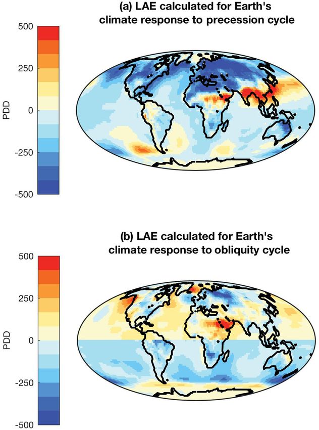
378          R. Roychowdhury and R. DeConto: Interhemispheric effect of global geography on Earth’s climate response

                                                                      Continental geography has a strong impact on polar cli-
                                                                   mates, as is evident from the very different climatic regimes
                                                                   of the Arctic and the Antarctic. Several early paleoclimate
                                                                   modeling studies using GCMs investigated continental dis-
                                                                   tribution as a forcing factor of global climate (e.g., Barron et
                                                                   al., 1984; Hay et al., 1990). These studies demonstrated that
                                                                   an Earth with its continents concentrated in the low latitudes
                                                                   is warmer and has lower Equator-to-pole temperature gradi-
                                                                   ents than an Earth with only polar continents. Although these
                                                                   early model simulations did not incorporate all of the com-
                                                                   plexities of the climate system, the results provided valuable
                                                                   insights from comparative studies of polar versus equatorial
                                                                   continents on the Earth and showed that changes in conti-
                                                                   nental configuration has a significant influence on climatic
                                                                   response to forcing.
                                                                      The asymmetry in the climates of the NH and SH can be
                                                                   attributed to three primary causes: (i) astronomical, i.e., vari-
                                                                   ation in insolation intensity across the NH and SH caused by
                                                                   the precession of the equinoxes (today’s perihelion coincides
                                                                   with 3 January, just after the 21 December solstice, leading
                                                                   to slightly stronger summer insolation in the SH); (ii) conti-
                                                                   nental geography, i.e., the effect of continental geography on
                                                                   climate as described above; and (iii) interhemispheric conti-
Figure 1. (a) Top-of-atmosphere net incoming radiation (annual     nental geography, i.e., the effect of NH continental geogra-
mean). (b) Mean summer temperatures (blue) and mean annual tem-    phy on SH climate and vice versa. The aim of this study is
peratures (green) computed from GCM simulations with a modern      to gain a better understanding and isolate the effect of inter-
orbit. (c) Positive degree days (PDDs) calculated from GCM simu-   hemispheric continental geography on climate by comparing
lations with a modern orbit.                                       results from GCM simulations using modern versus idealized
                                                                   (hemispherically symmetric) global geographies. The GCM
   The distribution of continents and oceans has an impor-         simulations with modern and idealized (symmetric) geogra-
tant effect on the spatial heterogeneity of the Earth’s energy     phies are used to quantify the different climate responses to
balance, primarily via the differences in albedos and ther-        a range of orbits. By comparing the climatic response from
mal properties of land versus ocean (Trenberth et al., 2009).      simulations with different geographies, we isolate and esti-
The latitudinal distribution of land has a dominant effect on      mate the effect of interhemispheric continental geography,
zonally averaged net radiation balance due to its influence        i.e., the influence of one hemisphere’s geography on the cli-
on planetary albedo and its ability to transfer energy to the      mate response of the opposite hemisphere.
atmosphere through long-wave radiation, and fluxes of sen-            One of the main caveats of this study is the lack of a dy-
sible and latent heat. The latitudinal net radiation gradient      namical ocean in our model setup. While this presents cer-
controls the total poleward heat transport requirement, which      tain limitations, the model’s computational efficiency has the
is the ultimate driver of winds and ocean circulation (Stone,      advantage of allowing for a wide range of orbital parame-
1978). Oceans have a relatively slower response to seasonal        ter space to be explored. We view the inclusion of a full-
changes in insolation due to the higher specific heat of water     depth dynamical ocean as a next step, hopefully motivated
as compared to land, and mixing in the upper ∼ 10–150 m of         in part by the results published here. Furthermore, dynami-
the ocean. As a result, in the ocean-dominated SH, the sur-        cal ocean models introduce an additional level of complexity
face waters suppress extreme temperature swings in the win-        and model dependencies that we think are best avoided in
ter and provide the atmosphere with a source of moisture and       this initial study.
diabatic heating. In the land-dominated NH, the lower heat
capacity of the land combined with relatively high albedo          2     Model
results in greater seasonality, particularly in the interiors of
large continents (Asia and North America). The land surface        2.1    Experimental design
available in a particular hemisphere also affects the poten-
tial for widespread glaciation, and the extreme cold winters       GCMs have been used to extensively study the importance
associated with large continents covered by winter snow.           of geography on the Earth’s climate in the past. In this study,
                                                                   we use the latest (2012) version of the Global ENvironmen-
                                                                   tal and Ecological Simulation of Interactive Systems (GEN-

Clim. Past, 15, 377–388, 2019                                                                  www.clim-past.net/15/377/2019/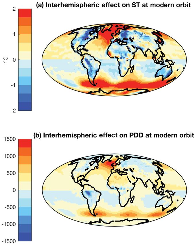
R. Roychowdhury and R. DeConto: Interhemispheric effect of global geography on Earth’s climate response 379
ESIS) 3.0 GCM with a slab ocean component (Thompson
and Pollard, 1997) rather than a full-depth dynamical ocean
(Alder et al., 2011). The slab ocean predicts sea surface tem-
peratures and ocean heat transport as a function of the local
temperature gradient and the zonal fraction of land versus
sea at each latitude. While explicit changes in ocean cur-
rents and the deep ocean are not represented, the computa-
tional efficiency of the slab ocean version of the GCM allows
for numerous simulations with idealized global geographies
and greatly simplifies interpretations of the sensitivity tests
by precluding complications associated with ocean model
dependencies. The ocean depth is limited to 50 m (enough
to capture the seasonal cycle of the mixed layer). In addi-
tion to the atmosphere and slab ocean, the GCM includes
model components representing vegetation, soil, snow and
thermodynamic sea ice. The 3-D atmospheric component of
the GCM uses an adapted version of the NCAR CCM3 solar
and thermal infrared radiation code (Kiehl et al., 1998) and is
coupled to the surface components by a land-surface-transfer
scheme. In the setup used here, the model atmosphere has a
spectral resolution of T31 (∼ 3.75◦ ) with 18 vertical layers.
Land-surface components are discretized on a higher resolu-
tion 2◦ × 2◦ grid.
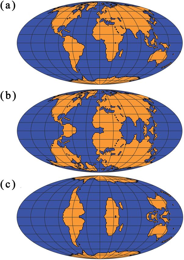
The GCM uses various geographical boundary conditions
(described below) in 2◦ × 2◦ and spectral T31 grids for sur- Figure 2. (a) modern continental geography, (b) NORTH-SYMM
face and atmospheric general circulation models (AGCMs), geography and (c) SOUTH-SYMM geography.
respectively. For each set of experiments, the model is run for
50 years. Spin-up is taken into account, and equilibrium is ef-
fectively reached after about 20 years of integration. The re- Equator into the SH. Similarly, in the experiment SOUTH-
sults used to calculate interhemispheric effects are averaged SYMM, the land mask and geographic boundary conditions
over the last 20 years of each simulation. Greenhouse-gas in the SH are mirrored in the NH. The NORTH-SYMM and
mixing ratios are identical in all experiments and set to prein- SOUTH-SYMM boundary conditions are shown in Fig. 2b
dustrial levels with CO2 set to 280 ppmv, N2 O to 288 ppbv and c with the CONTROL (Fig. 2a) for comparison. Pole-
and CH4 to 800 ppbv (Meinshausen et al., 2011). The default ward oceanic heat flux is defined as a function of the tem-
values for CFCl3 and CF2 Cl2 values are set to 0 ppm. The perature gradient and the zonal fraction of land and sea at a
solar constant is maintained at 1367 W m−2 . given latitude in the model; hence the parameterized ocean
heat flux is symmetric in our symmetrical Earth simulations.
2.2 Asymmetric and symmetric Earth geographies
3 Symmetry (and asymmetry) in GCM results
The GCM experiments are divided into three sets: (1) prein-
dustrial CONTROL, (2) NORTH-SYMM and (3) SOUTH- In the first experimental setup, we run the GCM with
SYMM. The preindustrial CONTROL experiments use modern-day orbital configuration, i.e., eccentricity is set
a modern global geography spatially interpolated to the to 0.0167, obliquity is set to 23.5◦ and precession such
model’s 2◦ × 2◦ surface grid (Cuming and Hawkins, 1981; that perihelion coincides with the SH summer. The top-of-
Kineman, 1985). The geographical inputs provide the land– atmosphere radiation is shown in terms of mean summer
ice sheet–ocean mask and land-surface elevations used by the insolation and summer energy (Fig. 3a and b). The sum-
GCM, along with global maps of vegetation distribution, soil mer energy is an integrated measure of changes in insolation
texture and other quantities (Koenig et al., 2012). intensity
To simulate the climate of an Earth with meridionally P as well as duration of summer, and is defined as
J = βi (Wi × 86 400), where Wi is mean insolation mea-
symmetric geographies, we created two sets of land-surface i
boundary conditions: NORTH-SYMM and SOUTH-SYMM. sured in W m−2 on day i, and β equals 1 when Wi ≥ τ and
For the NORTH-SYMM experiments, the CONTROL exper- 0 otherwise. τ = 275 W m−2 is taken as the threshold for
iment boundary conditions are used to generate a modified melting to start at the surface of the Earth. Mean summer
GCM surface mask, by reflecting the NH geography (land– temperature (ST) is calculated from the GCM as the mean
sea-ice mask, topography, vegetation, soil texture) across the of the average daily temperatures for the summer months in
www.clim-past.net/15/377/2019/ Clim. Past, 15, 377–388, 2019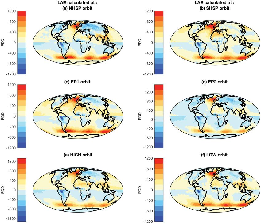
380          R. Roychowdhury and R. DeConto: Interhemispheric effect of global geography on Earth’s climate response

Figure 3. (a–d) Demonstration of Earth’s asymmetric climate response to symmetric climate forcing. Simulations are forced with modern
orbit: (a) summer insolation; (b) summer energy (as defined in Huybers, 2006); (c) summer temperature; and (d) PDD. (e–h) Demonstration
of Earth’s symmetric climate response to climate forcing when idealized symmetric Earth geographies are used. Simulations are forced by
modern-day orbit: (e, f) summer temperature and PDD for NORTH-SYMM simulation, (g, h) summer temperature and PDD for SOUTH-
SYMM simulation. The zonal averages are plotted on the right of each panel. Zonal averages of PDD are plotted on a log scale.

each hemisphere. We define summer by an insolation thresh-            ric continents make the climates of the NH and SH symmet-
old (325 W m−2 ) that accounts for the astronomical posi-             ric (> 95 %). However, due to the current timing of perihe-
tions as well as the phasing of the seasonal cycle of inso-           lion with respect to the summer solstices, there remains some
lation. The zonal averages of ST (calculated at each latitude)        minor asymmetry. Using an orbit in which perihelion coin-
demonstrate the inherent asymmetry in the Earth’s climate             cides with equinoxes will make the climate truly symmetri-
between NH and SH, especially evident in the higher lati-             cal.
tudes (Fig. 3c). Positive degree days (PDDs) capture the in-
tensity as well as the duration of the melt season, and have
                                                                      4     Modern orbit simulations
been shown to be indicative of the ice-sheet response to
changes in external forcing. Figure 3d shows the PDDs for             4.1    Effect of SH on NH climate
modern orbit, with zonal averages plotted on the log scale.
The asymmetry between the NH and SH is captured by the                To estimate the effect of SH continental geography on
GCM in the calculated PDDs.                                           NH climate, we subtract the NH climate of the NORTH-
   Next, we maintain the modern orbit to test the effect of           SYMM simulation (symmetric NH continents in both hemi-
meridionally symmetric continents (Fig. 3e–h). Figure 3e              spheres) from the CONTROL simulation (asymmetric, mod-
and f shows ST and PDD from a simulation in which the NH              ern orbit). In these two simulations, the only difference in
geography is reflected in the SH (thus making the Earth geo-          setup is the SH continental distribution. Thus the differ-
graphically symmetric). Figure 3g and h shows ST and PDD              ence in NH climate from the two simulations, if any, can be
from the simulation with symmetric SH continents. Symmet-             safely ascribed as the effect of SH continental geography on
                                                                      NH climate. We quantify this interhemispheric effect for ST

Clim. Past, 15, 377–388, 2019                                                                     www.clim-past.net/15/377/2019/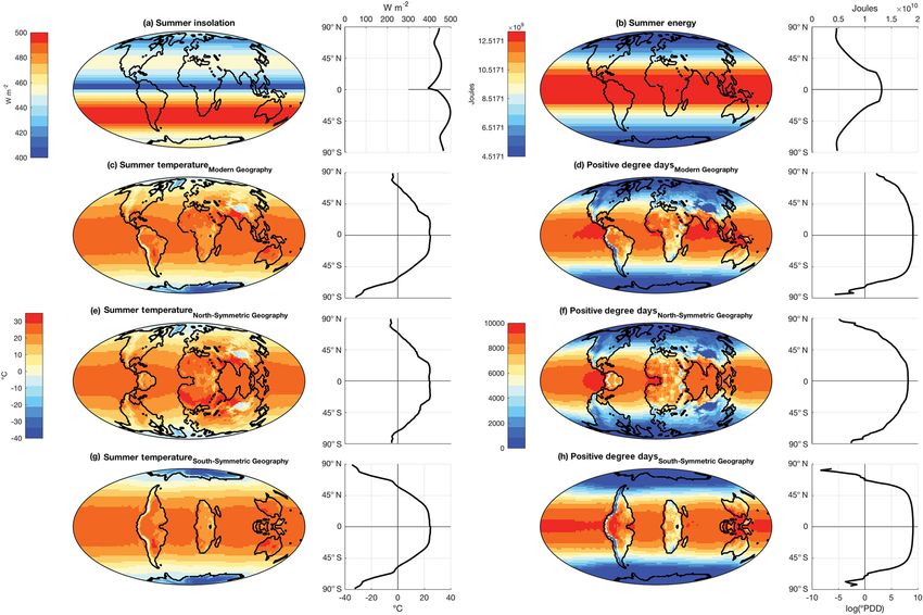
R. Roychowdhury and R. DeConto: Interhemispheric effect of global geography on Earth’s climate response                    381

(for NH) as
                    n
                  1X
êSummer Temp =         Ticontrol − Tinorth .             (1)
                  n i

Analogous to the effect for ST, the effect for PDD, which
we call the “Land Asymmetry Effect” (LAE), is defined as
follows:

LAE(NH) = PDDcontrol − PDDnorth ,                         (2)

where Ticontrol and PDDcontrol are the mean daily temperature
and PDD from the CONTROL simulation, and Tinorth and
PDDnorth are the mean daily temperature and PDD from the
simulation with the North-Symmetric configuration geogra-
phy (NORTH-SYMM). n is the number of days in the sum-
mer months in each hemisphere.

4.2   Effect of NH on SH climate
Similarly, we estimate the effect of NH continental geogra-
phy on the SH by subtracting the SH climate of the SOUTH-
SYMM simulation (symmetric southern continents in both
                                                                Figure 4. Interhemispheric effect of continental geography on
hemispheres) from the CONTROL simulation (asymmetric,
                                                                (a) mean summer temperature (ST) and (b) positive degree
modern orbit). In these two simulations, the differences in     days (PDD).
SH climate in the CONTROL and SOUTH-SYMM simula-
tions, if any, can be ascribed as the “effect of NH continen-
tal geography on SH climate”. We quantify this interhemi-          For the SH, the STs are calculated when the insolation is
spheric effect for ST (for SH) and the LAE as                   most intense over the SH during the year. SH landmasses,
                    n                                          except Antarctica, generally show a cooling response dur-
                  1X
                                                                ing summer, due to NH geography. Over Antarctica, STs
êSummer Temp =         Ticontrol − Tisouth ,             (3)
                  n i                                           are higher in the control simulations than in the symmetric
LAESH = PDDcontrol − PDDsouth ,                           (4)   simulations, leading to the inference that there is a warm-
                                                                ing (increase) in STs due to interhemispheric effect. Also,
where Ticontrol and PDDcontrol are the mean daily temperature   the Southern Ocean shows a strong positive temperature ef-
and PDD from the CONTROL simulation, and Tisouth and            fect (warming) relative to a symmetric Earth, although this
PDDsouth are the mean daily temperature and PDD from the        Southern Ocean response might be different or modified if a
simulation with the South-Symmetric configuration geogra-       full-depth dynamical ocean model was used.
phy (SOUTH-SYMM).
                                                                5   Idealized orbit simulations
4.3   Results of modern orbit simulations
                                                                Next, we examine the effect of the opposite hemisphere on
Figure 4a and b shows the interhemispheric effect of conti-     the Earth’s climate response at extreme obliquities (axial tilt)
nental geography on ST and PDD, respectively. For the NH,       and idealized precessional configurations (positions of the
the STs are calculated when the insolation intensity over the   solstices and equinoxes in relation to the eccentric orbit).
NH is strongest. The asymmetry in the SH landmasses leads       The orbital parameters used in these experiments are ide-
to weakening of the summer warming over North America           alized and do not correspond to a specific time in Earth’s
and Eurasia (blue shaded regions correspond to cooling).        history. Rather, they are chosen to provide a useful frame-
Consequently, STs over NH continents are lower by 3–6 ◦ C       work for studying the Earth’s climate response to preces-
relative to a symmetric Earth. There is a positive warming      sion and obliquity. HIGH and LOW orbits approximate the
effect in the North-Atlantic Ocean, and in general the NH       highest and lowest obliquity in the last 3 million years
oceans are slightly warmer relative to a symmetric Earth. The   (Berger and Loutre, 1991). NHSP (NH summer at perihe-
general trends in the interhemispheric effect on PDD (LAE)      lion) and SHSP (SH Summer at Perihelion) orbits corre-
(Fig. 4b) mimic those of the STs (Fig. 4a).                     spond to NH and SH summers coinciding with perihelion,
                                                                respectively. The other two precessional configurations con-

www.clim-past.net/15/377/2019/                                                                Clim. Past, 15, 377–388, 2019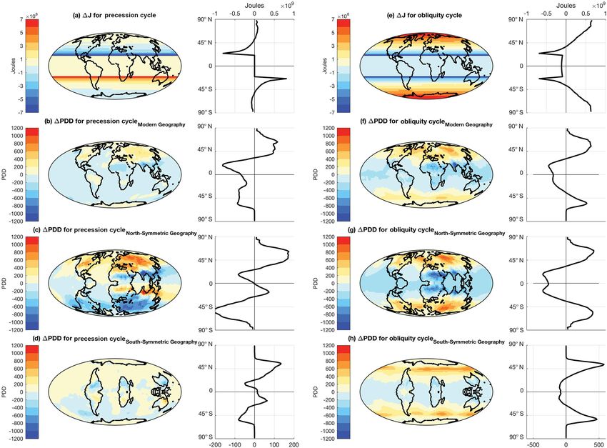
382          R. Roychowdhury and R. DeConto: Interhemispheric effect of global geography on Earth’s climate response

Table 1. Experimental setup of model boundary conditions and forcings.

                Run ID                          LSX1 configuration            Eccentricity        Obliquity       Precession2              GHGs3
                CONTROLNHSP                     Modern                            0.034            23.2735        270◦ (NHSP)           preindustrial
                CONTROLSHSP                     Modern                            0.034            23.2735        90◦ (SHSP)            preindustrial
                CONTROLEP1                      Modern                            0.034            23.2735        0◦ (EP1)              preindustrial
                CONTROLEP2                      Modern                            0.034            23.2735        180◦ (EP2)            preindustrial
                CONTROLHIGH                     Modern                            0.034            24.5044        180◦                  preindustrial
                CONTROLLOW                      Modern                            0.034            22.0425        180◦                  preindustrial
                NORTH-SYMMNHSP                  North-Symmetric                   0.034            23.2735        270◦ (NHSP)           preindustrial
                NORTH-SYMMSHSP                  North-Symmetric                   0.034            23.2735        90◦ (SHSP)            preindustrial
                NORTH-SYMMEP1                   North-Symmetric                   0.034            23.2735        0◦ (EP1)              preindustrial
                NORTH-SYMMEP2                   North-Symmetric                   0.034            23.2735        180◦ (EP2)            preindustrial
                NORTH-SYMMHIGH                  North-Symmetric                   0.034            24.5044        180◦                  preindustrial
                NORTH-SYMMLOW                   North-Symmetric                   0.034            22.0425        180◦                  preindustrial
                SOUTH-SYMMNHSP                  South-Symmetric                   0.034            23.2735        270◦ (NHSP)           preindustrial
                SOUTH-SYMMSHSP                  South-Symmetric                   0.034            23.2735        90◦ (SHSP)            preindustrial
                SOUTH-SYMMEP1                   South-Symmetric                   0.034            23.2735        0◦ (EP1)              preindustrial
                SOUTH-SYMMEP2                   South-Symmetric                   0.034            23.2735        180◦ (EP2)            preindustrial
                SOUTH-SYMMHIGH                  South-Symmetric                   0.034            24.5044        180◦                  preindustrial
                SOUTH-SYMMLOW                   South-Symmetric                   0.034            22.0425        180◦                  preindustrial
              NHSP: NH summer solstice at perihelion; SHSP: SH summer solstice at perihelion; EP1: NH vernal equinox at perihelion and EP2: NH
              autumnal equinox at perihelion. 1 LSX represents the land-surface transfer scheme. 2 Orbital precession in the GCM is defined here as the
              prograde angle from perihelion to the NH vernal equinox. 3 GHGs represents greenhouse gases.

sidered are EP1 and EP2, with the perihelion coinciding with                           duction in the tilt from 24.5◦ (HIGH) to 22◦ (LOW) re-
the equinoxes. For the idealized precession simulations, the                           duces annual insolation by ∼ 17 W m−2 and summer inso-
obliquity is set to its mean value averaged over the last 3 mil-                       lation by ∼ 45 W m−2 in the high latitudes. In the tropics,
lion years. Eccentricity is set to the same moderate value                             summer insolation increases by up to ∼ 5 W m−2 . Loutre et
(mean eccentricity over the last 3 million years) for all sim-                         al. (2004), among others, predicted that global ice volume
ulations. Table 1 summarizes the orbits used in the ensem-                             changes at the obliquity periods could be interpreted as a re-
ble of model simulations. Here, we focus only on the LAE,                              sponse to mean annual insolation and meridional insolation
as PDD is a better indicator of air temperature’s influence                            gradients. To demonstrate asymmetry in the climate response
on annual ablation over ice sheets than ST, since this metric                          to obliquity, we take the differences between the highest and
captures both the intensity and duration of the melt season.                           lowest obliquities for both the forcing and the climate re-
   Changes in precession primarily affect seasonal insolation                          sponse. The difference in the PDDs (1PDDobliquity ) is the
intensity that is well known to be out of phase in both hemi-                          Earth’s climate response to changes in tilt. Figure 5f shows
spheres (Lyell, 1832). To demonstrate an asymmetry in the                              1PDDobliquity and the zonal averages reveal the asymme-
climate response to precession, we take the differences be-                            try in the obliquity climate response. The same simulations
tween two arbitrarily chosen extremes in the precession cy-                            with North-Symmetric Earth (Fig. 5g) and South-Symmetric
cle (NHSP and SHSP) for both the forcing and the climate                               Earth (Fig. 5h) produce symmetrical climate responses to the
response. The forcing (summer energy – J) calculated at the                            obliquity cycle.
top of the atmosphere is numerically symmetric (but out of
phase as expected) in both hemispheres (Fig. 5a). The dif-                             6    Results of idealized orbit simulations
ference in the PDDs (1PDDprecession ) is the Earth’s climate
response to the combined effect of the two precessional mo-                            The effect of SH continental geography on NH at the ide-
tions (wobbling of the axis of rotation and the slow turning                           alized orbits is estimated using the same method described
of the orbital ellipse). The climate response (1PDDprecession )                        above, with the LAE for a given orbit (for NH) calculated as
is asymmetric across both hemispheres (Fig. 5b). However,
when we run the precessional simulations in an Earth with                              LAE(NH) = PDDcontrol    north
                                                                                                    orbit − PDDorbit .                                    (5)
symmetric continents, the climate response to precession is
                                                                                       Similarly, the effect of NH continental geography on SH at
symmetrical (Fig. 5c and d).
                                                                                       the idealized orbits is estimated using the same method de-
   In contrast to precession, obliquity alters the seasonality
                                                                                       scribed above, with the LAE for a given orbit (for SH) calcu-
of insolation equally in both hemispheres (Fig. 5e). A re-
                                                                                       lated as

Clim. Past, 15, 377–388, 2019                                                                                                www.clim-past.net/15/377/2019/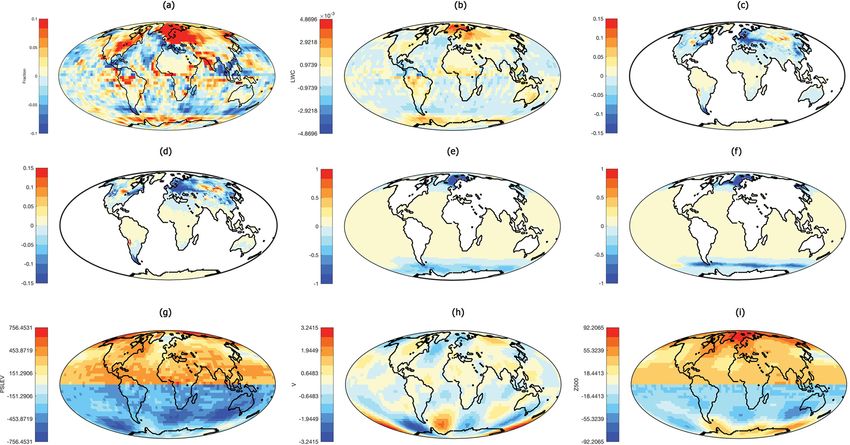
R. Roychowdhury and R. DeConto: Interhemispheric effect of global geography on Earth’s climate response                        383

Figure 5. Summer energy (J) change for a transition from a SHSP to a NHSP orbit (a); and the corresponding change in positive degree
days (PDD) in CONTROL (b); NORTH-SYMM (c) and SOUTH-SYMM (d) simulations. Summer energy (J) change for a transition from
LOW to HIGH orbit (e); and the corresponding change in PDD in CONTROL (f); NORTH-SYMM (g) and SOUTH-SYMM (h) simulations.

                                                                    spheric effect dampens the magnitude of “glacial” versus “in-
LAE(SH) = PDDcontrol    south
             orbit − PDDorbit .                             (6)     terglacial” conditions in both hemispheres.
                                                                       Figure 6b shows the spatial variation in LAE when perihe-
Figure 6a shows the spatial variation in LAE when perihelion        lion coincides with SH summer (SHSP). The NH continents
coincides with NH summer (NHSP). The NH landmasses                  have a weak positive effect, leading to slightly warmer con-
show a strong negative response. In this orbit, the NH experi-      ditions relative to a symmetric Earth. In this orbit, the south-
ences elevated summer insolation, but the response is attenu-       ern high latitudes experience intense summer insolation. The
ated by the interhemispheric effect. This dampening effect is       positive warming effect amplifies the already warm condi-
greatest in the interiors of the NH continents. If precession is    tions in the SH. Figure 6c and d shows the spatial variation
considered in isolation (i.e., constant obliquity), then accord-    in LAE at the two equinoxes, i.e., when NH vernal equinox is
ing to the astronomical theory of climate the NH should ex-         at perihelion (EP1) and when NH autumnal equinox is at per-
perience “interglacial” conditions when perihelion coincides        ihelion (EP2). The LAE is in general weaker at the equinoxes
with NH summer. However, because of the interhemispheric            than at the solstices.
effect, interglacial (warm summer) conditions are muted rel-           At HIGH obliquity, there exists a negative effect on NH
ative to those on a symmetric Earth. During this orbit, the         continents (Fig. 6e), which mutes the strong insolation inten-
SH experiences “glacial” (cold summer) conditions due to            sity during summer months. In the NH, as a result of conti-
the weaker summer insolation. The positive effect in the SH         nental asymmetry, a decrease in the Equator-to-pole temper-
leads to weaker cooling relative to a symmetric Earth. Thus,        ature gradient is observed. A lowering of STs and tempera-
when perihelion coincides with NH summer, the interhemi-

www.clim-past.net/15/377/2019/                                                                    Clim. Past, 15, 377–388, 2019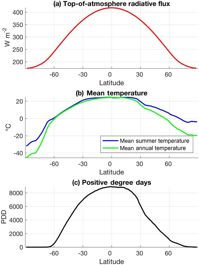
384          R. Roychowdhury and R. DeConto: Interhemispheric effect of global geography on Earth’s climate response

Figure 6. Interhemispheric effect of continental geography (LAE) on the climate response (PDD) at (a) NH summer at perihelion; (b) SH
summer at perihelion; (c) NH vernal equinox at perihelion; (d) NH autumnal equinox at perihelion; (e) HIGH obliquity orbit; and (f) LOW
obliquity orbit.

ture gradient due to the interhemispheric effect has a nega-          7   LAE for orbital cycles
tive impact on the deglaciation trigger associated with HIGH
obliquity orbits. Thus the interhemispheric effect would hin-         Next, we calculate the LAE for a transition through a preces-
der the melting of ice during high-obliquity orbits. In the SH,       sional cycle. We take two arbitrary end points in the preces-
the positive interhemispheric effect on PDD over Antarctica           sional cycle (NHSP and SHSP) and calculate the difference
and the Southern Ocean leads to overall higher temperatures           of PDDs between the two simulations (1PDDprecession_cycle ).
in the southern high latitudes as compared to a symmetric             The LAE for precessional cycle is therefore calculated as
Earth. Thus, during the HIGH obliquity orbits the positive
effect helps deglaciation.                                            LAE(NH) = 1PDDcontrol                north
                                                                                    precession_cycle − 1PDDprecession_cycle , (7)
   At LOW obliquity, the negative effect over NH continents
is generally less intense (Fig. 6f). However, even the modest         LAE(SH) = 1PDDcontrol                south
                                                                                    precession_cycle − 1PDDprecession_cycle . (8)
lowering of summer temperatures caused by the interhemi-
spheric effect would support the growth of ice sheets dur-            The LAE shows a strong negative effect in the NH (Fig. 7a).
ing low-obliquity orbits. The positive effect (warming) in the        For the NH, this transition from SHSP to NHSP equates to a
southern high latitudes would delay the growth of ice sheets.         transition from a cool to a warm climate. The negative inter-
                                                                      hemispheric effect decreases the |1PDD| in the real Earth,
                                                                      thus weakening the effect of precession in the NH. The SH
                                                                      shows a positive effect on PDD at high latitudes. For the
                                                                      SH, the transition from SHSP to NHSP equates to a transi-
                                                                      tion from warmer to cooler climate. The positive interhemi-
                                                                      spheric effect at high latitudes decreases the |1PDD| in the

Clim. Past, 15, 377–388, 2019                                                                     www.clim-past.net/15/377/2019/
R. Roychowdhury and R. DeConto: Interhemispheric effect of global geography on Earth’s climate response 385
8 Impact of various climatological variables on LAE
A comprehensive, mechanistic evaluation of the interhemi-
spheric effect is beyond the scope of this initial study. How-
ever, as a first step, we test the relationship between the hemi-
spheric LAE and various atmospheric processes by explor-
ing correlations between the interhemispheric responses to
orbital forcing, and climatological fields related to changes
in radiation (clouds), dynamics (heat and moisture conver-
gence) and feedbacks related to surface processes (sea ice
and snow albedos).
Numerous studies have shown the impact of variation in
the distribution of clouds on climate (e.g., Meleshko and
Wetherald, 1981). It is observed that the cloud cover alters
in idealized symmetric continent experiments, i.e., the hemi-
spheric asymmetry in the continental geography impacts the
distribution of cloud cover (cloud cover is measured as the
mean of total cloudiness). Cloud cover affects the climate
through two opposing influences; a cooling effect is pro-
duced due to reflection of solar radiation, and a warming
effect on climate due to reduction of effective temperature
for outgoing terrestrial (long-wave) radiation (Wetherald et
al., 1980). However, the overall effect of increasing cloud
Figure 7. Interhemispheric effect of continental geography on the cover is generally considered to cause cooling (Manabe et
climate response to (a) precession cycle (SHSP to NHSP); and al., 1967; Schneider, 1972). The hemispheric asymmetry im-
(b) obliquity cycle (LOW to HIGH). pacts the cloud cover fraction by as much as 10 % at var-
ious latitudes (Fig. 8a). The effect of asymmetry increases
cloudiness over land poleward of 50◦ N latitude, contributing
to negative net radiation and temperature anomalies over the
real Earth, thus weakening the effect of precessional cycle in NH continents, and this can be observed both in terms of ST
the SH high latitudes. and the PDD. In the SH, total cloudiness decreases over the
To calculate the LAE for a transition through the obliq- Southern Ocean due to hemispheric asymmetry, contributing
uity cycle, we take the highest and lowest obliquities (HIGH to a positive temperature anomaly over this region. At lati-
and LOW), and calculate the difference of PDDs between the tudes below 50◦ , the increase in the area-mean flux of out-
two simulations (1PDDobliquity_cycle ). The LAE for obliquity going terrestrial radiation is almost compensated by the in-
cycle is therefore calculated as crease in net insolation flux. Thus, we expect a minor impact
of cloud content on the LAE at lower latitudes.
Snow cover reflects ∼ 80 % to 90 % of the Sun’s energy
LAE(NH) = 1PDDcontrol north
obliquity_cycle − 1PDDobliquity_cycle , (9) and it has an important influence on energy balance and re-
LAE(SH) = 1PDDcontrol south
(10) gional water budgets. Snow cover’s effect on surface energy
obliquity_cycle − 1PDDobliquity_cycle .
balance has a strong cooling effect; and conversely, decreas-
ing snow cover leads to a decrease in surface albedo and
The NH shows a small negative effect in the high latitudes, warming. We find that the snow fraction (annual and monthly
and a positive effect in the low latitudes (Fig. 7b). The tran- averages) is also influenced by the hemispheric asymmetry
sition from LOW to HIGH corresponds to a transition from of the continents. There is a decrease in the snow fraction
cold to warm climate. The negative interhemispheric effect over most of Eurasia and North America due to hemispheric
decreases the 1PDD, thus weakening the climate response asymmetry (Fig. 8c), leading to warming in the asymmetrical
of the obliquity cycle in the high latitudes. The positive inter- Earth when compared to an Earth with symmetric continents.
hemispheric effect increases the 1PDD, thus strengthening The effect is more pronounced in the spring months (Fig. 8d),
the climate response of obliquity cycle in the low latitudes in which leads to longer summers, increasing the PDDs in the
the NH. The SH largely shows a negative effect, with a pos- asymmetric Earth. The relationship between the snow frac-
itive effect in the high latitudes. The transition from LOW to tion and temperature anomalies is expected to be weaker in
HIGH corresponds to a transition from cold to warm climate. the heavily forested regions (such as Northern Asia), where
The positive interhemispheric effect increases the 1PDD, the snow–albedo feedback is less effective (Bonan et al.,
thus amplifying the effect of obliquity over Antarctica. 1992). Similarly, fractional sea-ice cover has an opposing ef-
www.clim-past.net/15/377/2019/ Clim. Past, 15, 377–388, 2019386 R. Roychowdhury and R. DeConto: Interhemispheric effect of global geography on Earth’s climate response
Figure 8. The effect of interhemispheric continental distribution on (a) mean annual cloud cover fraction, (b) liquid water content from all
cloud types (kg kg−1 ), (c) fractional snow cover (annual mean), (d) fractional snow cover (averaged over spring months), (e) fractional sea-
ice cover (annual mean), (f) fractional sea-ice cover (averaged over spring months), (g) sea level pressure (Pa, annual mean), (h) northward
wind (m s−1 , annual mean) and (i) 500 hPa geopotential height (m, annual mean).
fect on temperature. Thus, an increase in fractional sea-ice Friedman, 2012; Harnack and Harnack, 1985; Hou, 1998; Ji
cover due to hemispheric asymmetry causes a negative LAE, et al., 2014). However, far-field effects such as those arising
as increased albedo reduces net short-wave radiative flux. from interactions between the Hadley circulation and plan-
Spatial patterns in the LAE are compared with basic dy- etary waves (among other dynamical processes) are not ad-
namical effects of the different geographies. Sea level pres- equately resolved at the relatively coarse spatial resolution
sure shows an effect due to hemispheric asymmetry (Fig. 8g), used in these initial simulations, with monthly meteorologi-
with a general increase in the NH and a decrease in the cal output. A more complete dynamical analysis of the LAE
SH. The resulting change in the time-averaged (mean an- is the subject of ongoing work and a future paper.
nual shown here) wind field can be seen in northward winds
(Fig. 8h) and imply a dynamical contribution to the LAE
anomaly patterns via warm air advection. Spatial patterns in 9 Conclusions
these dynamical linkages can help explain some of the re-
gional anomalies seen in the LAE. For example, we find re- The unbalanced fraction of land in the NH versus SH has
duced winds in the North Atlantic leading to reduced heat remained almost unchanged for tens of millions of years.
loss out of that region. This hints at a tropical teleconnection However, the significance of this continental asymmetry on
to the westerlies (e.g., Hou, 1998), propagating the impact Earth’s climate response to forcing has not been previously
of low-latitude geography to the midlatitudes of the opposite quantified with a physically based climate model. We find
hemisphere, in this case with an amplifying impact on sea that continental geography of the opposite hemisphere has a
ice and regional warming in the North Atlantic. We observe control on the climate system’s response to insolation forc-
a positive relationship between the LAE and 500 hPa geopo- ing, and this may help explain the nonlinear response of the
tential height (Fig. 8i), whereby a positive “Z500 effect” indi- Earth’s climate to insolation forcing.
cates that the geopotential heights are regionally higher (im- According to classical Milankovitch theory, the growth of
plying warm temperatures across the region) when compared polar ice sheets at the onset of glaciation requires cooler sum-
to a symmetric Earth, and vice versa. Interhemispheric tele- mers in the high latitudes in order for snow to persist through-
connections like these have been extensively studied with out the year. During warm summers at the high latitudes, the
respect to present-day continental geography (Chiang and winter snowpack melts, inhibiting glaciation or leading to
deglaciation if ice sheets already exist. Thus, the intensity of
Clim. Past, 15, 377–388, 2019 www.clim-past.net/15/377/2019/R. Roychowdhury and R. DeConto: Interhemispheric effect of global geography on Earth’s climate response 387
summer insolation at high latitudes, especially the NH polar Acknowledgements. We thank anonymous reviewers for giving
latitudes, has been considered the key driver of the glacial– constructive comments towards the critical development of this pa-
interglacial cycles and other long-term climatic variations. per. We thank David Pollard for his help with the GCM simulations.
At precessional periods, at which the high-latitude summer
insolation intensity primarily varies (Huybers, 2006; Raymo Edited by: Pascale Braconnot
Reviewed by: three anonymous referees
et al., 2006, etc.), the land asymmetry effect plays an impor-
tant role by amplifying (and weakening at certain times) the
effect of summer insolation intensity.
In all the orbital configurations simulated here, we find that References
the geography of the SH weakens the temperature response
of the high NH latitudes to orbital forcing. Consequently, this Alder, J. R., Hostetler, S. W., Pollard, D., and Schmittner, A.: Eval-
leads to a larger latitudinal gradient in STs in the NH com- uation of a present-day climate simulation with a new coupled
pared to that of a symmetric Earth. In particular, the amplifi- atmosphere-ocean model GENMOM, Geosci. Model Dev., 4,
cation (or weakening) of the response to insolation changes 69–83, https://doi.org/10.5194/gmd-4-69-2011, 2011.
at precessional and obliquity periods might explain some of Barron, E. J., Thompson, S. L., and Hay, W. W.: Continental dis-
tribution as a forcing factor for global-scale temperature, Nature,
the important features of late Pliocene–early Pleistocene cli-
310, 574–575, https://doi.org/10.1038/310574a0, 1984.
mate variability, when obliquity-paced cyclicity dominated Berger, A. and Loutre, M. F.: Insolation values for the climate of
precession in global benthic δ 18 O records. In Fig. 7, we have the last 10 million years, Quaternary Sci. Rev., 10, 297–317,
demonstrated that the interhemispheric effect causes a sup- https://doi.org/10.1016/0277-3791(91)90033-Q, 1991.
pression of the effects of precessional cycle on the Earth’s Bonan, G. B., Pollard, D., and Thompson, S. L.: Effects of bo-
surface. In other words, the real Earth has a smaller response real forest vegetation on global climate, Nature, 359, 716–718,
to a precession cycle as compared to the hypothetical sym- https://doi.org/10.1038/359716a0, 1992.
metric Earth. We have also showed that the interhemispheric Chiang, J. C. H. and Friedman, A. R.: Extratropical Cool-
effect causes an amplification of the effects of obliquity cy- ing, Interhemispheric Thermal Gradients, and Tropical Cli-
cle on the Earth’s surface. In other words, the real Earth has a mate Change, Annu. Rev. Earth Planet. Sci., 40, 383–412,
larger response to the obliquity cycle in the ocean-dominated https://doi.org/10.1146/annurev-earth-042711-105545, 2012.
Roychowdhury, R. and DeConto, R. M.: Interhemispheric
SH, as compared to the hypothetical symmetric Earth. Con-
Effect of Global Geography on Earth’s Climate Re-
sequently, the interhemispheric effect of continental geogra-
sponse to Orbital Forcing (GCM Outputs), Mendeley Data,
phy contributes to the muting of precessional signal and am- https://doi.org/10.17632/kt8v7ths6p.1, 2019.
plification of obliquity signal recorded in paleoclimate prox- Croll, J.: On ocean-currents, part I: ocean-currents in relation to the
ies such as benthic δ 18 O isotope records. distribution of heat over the globe, Philos. Mag. J. Sci., 39, 81–
There are various ways in which the Earth’s continen- 106, 1870.
tal asymmetry affects climate. Here, we have shown how Cuming, M. J. and Hawkins, B. A.: TERDAT: The FNOC sys-
these interhemispheric effects influence the Earth’s climate tem for terrain data extraction and processing, Tech. Rep. M11
response to orbital forcing via the radiative and atmospheric Project M254, 2nd Edn., US Navy Fleet Numerical Oceanogra-
dynamical processes represented in a slab ocean GCM. phy Center, Monterey, CA, 1981.
While computationally challenging, future work should in- Deconto, R. M., Pollard, D., Wilson, P. A., Pälike, H., Lear, C. H.,
and Pagani, M.: Thresholds for Cenozoic bipolar glaciation, Na-
clude complimentary simulations with atmosphere–ocean
ture, 455, 652–656, https://doi.org/10.1038/nature07337, 2008.
general circulation models to explore the potential modify-
Flato, G. M. and Boer, G. J.: Warming asymmetry in cli-
ing role of ocean dynamics on the amplifying and weakening mate change simulations, Geophys. Res. Lett., 28, 195–198,
interhemispheric responses to orbital forcing demonstrated https://doi.org/10.1029/2000GL012121, 2001.
here. Harnack, R. P. and Harnack, J.: Intra- and inter-
hemispheric teleconnections using seasonal southern
hemisphere sea level pressure, J. Climatol., 5, 283–296,
Data availability. The GENESIS GCM model out- https://doi.org/10.1002/joc.3370050305, 1985.
put that was generated for this study is archived under Hay, W. W., Barron, E. J., and Thompson, S. L.: Results of global
https://doi.org/10.17632/kt8v7ths6p.1 (Roychowdhury and atmospheric circulation experiments on an Earth with a merid-
DeConto, 2019). ional pole-to-pole continent, J. Geol. Soc. Lond., 147, 385–392,
https://doi.org/10.1144/gsjgs.147.2.0385, 1990.
Hou, A. Y.: Hadley Circulation as a Modula-
Competing interests. The authors declare that they have no con- tor of the Extratropical Climate, J. Atmos.
flict of interest. Sci., 55, 2437–2457, https://doi.org/10.1175/1520-
0469(1998)0552.0.CO;2, 1998.
Huybers, P.: Early Pleistocene glacial cycles and the inte-
grated summer insolation forcing, Science, 313, 508–511,
https://doi.org/10.1126/science.1125249, 2006.
www.clim-past.net/15/377/2019/ Clim. Past, 15, 377–388, 2019388 R. Roychowdhury and R. DeConto: Interhemispheric effect of global geography on Earth’s climate response
Ji, X., Neelin, J. D., Lee, S.-K., Mechoso, C. R., Ji, X., Neelin, J. Meleshko, V. P. and Wetherald, R. T.: The effect of a geographi-
D., Lee, S.-K., and Mechoso, C. R.: Interhemispheric Telecon- cal cloud distribution on climate: A numerical experiment with
nections from Tropical Heat Sources in Intermediate and Simple an atmospheric general circulation model, J. Geophys. Res., 86,
Models, J. Climate, 27, 684–697, https://doi.org/10.1175/JCLI- 11995, https://doi.org/10.1029/JC086iC12p11995, 1981.
D-13-00017.1, 2014. Philander, S. G. H., Gu, D., Lambert, G., Li, T.,
Kang, S. M., Seager, R., Frierson, D. M. W., and Liu, X.: Halpern, D., Lau, N.-C., and Pacanowski, R. C.:
Croll revisited: Why is the northern hemisphere warmer than Why the ITCZ Is Mostly North of the Equator, J.
the southern hemisphere?, Clim. Dynam., 44, 1457–1472, Climate, 9, 2958–2972, https://doi.org/10.1175/1520-
https://doi.org/10.1007/s00382-014-2147-z, 2014. 0442(1996)0092.0.CO;2, 1996.
Kiehl, J. T., Hack, J. J., Bonan, G. B., Boville, B. A., Raymo, M. E., Lisiecki, L. E., and Nisancioglu, K. H.: Plio-
Williamson, D. L., and Rasch, P. J.: The National Cen- Pleistocene Ice Volume, Antarctic Climate, and the Global δ 18 O
ter for Atmospheric Research Community Climate Model: Record, Science, 313, 492–495, 2006.
CCM3, J. Climate, 11, 1131–1149, https://doi.org/10.1175/1520- Schneider, S. H.: Cloudiness as a Global Climatic Feed-
0442(1998)0112.0.CO;2, 1998. back Mechanism: The Effects on the Radiation Balance
Kineman, J.: FNOC/NCAR global elevation, terrain, and surface and Surface Temperature of Variations in Cloudiness, J.
characteristics, Digital Dataset, 28 MB, NOAA National Geo- Atmos. Sci., 29, 1413–1422, https://doi.org/10.1175/1520-
physical Data Center, Boulder, 1985. 0469(1972)0292.0.CO;2, 1972.
Koenig, S. J., DeConto, R. M., and Pollard, D.: Pliocene Short, D. A., Mengel, J. G., Crowley, T. J., Hyde, W. T., and North,
Model Intercomparison Project Experiment 1: implemen- G. R.: Filtering of Milankovitch Cycles by Earth’s Geography,
tation strategy and mid-Pliocene global climatology us- Quaternary Res., 35, 157–173, https://doi.org/10.1016/0033-
ing GENESIS v3.0 GCM, Geosci. Model Dev., 5, 73–85, 5894(91)90064-C, 1991.
https://doi.org/10.5194/gmd-5-73-2012, 2012. Stone, P. H.: Constraints on dynamical transports of energy
Loutre, M.-F., Paillard, D., Vimeux, F., and Cortijo, E.: Does mean on a spherical planet, Dyn. Atmos. Ocean., 2, 123–139,
annual insolation have the potential to change the climate?, https://doi.org/10.1016/0377-0265(78)90006-4, 1978.
Earth Planet. Sc. Lett., 221, 1–14, https://doi.org/10.1016/S0012- Stouffer, R. J., Manabe, S., and Bryan, K.: Interhemispheric asym-
821X(04)00108-6, 2004. metry in climate response to a gradual increase of atmospheric
Lyell, C.: Principles of Geology, John Murray, Albemarle CO2 , Nature, 342, 660–662, https://doi.org/10.1038/342660a0,
Street, London, available at: https://www.bl.uk/collection-items/ 1989.
charles-lyells-principles-of-geology# (last access: 31 Jan- Thompson, S. L. and Pollard, D.: Greenland and Antarc-
uary 2018), 1832. tic Mass Balances for Present and Doubled Atmospheric
Manabe, S., Wetherald, R. T., Manabe, S., and Wether- CO2 from the GENESIS Version-2 Global Climate Model,
ald, R. T.: Thermal Equilibrium of the Atmosphere J. Climate, 10, 871–900, https://doi.org/10.1175/1520-
with a Given Distribution of Relative Humidity, J. At- 0442(1997)0102.0.CO;2, 1997.
mos. Sci., 24, 241–259, https://doi.org/10.1175/1520- Trenberth, K. E., Fasullo, J. T., Kiehl, J., Trenberth, K.
0469(1967)0242.0.CO;2, 1967. E., Fasullo, J. T., and Kiehl, J.: Earth’s Global En-
Meinshausen, M., Smith, S. J., Calvin, K., Daniel, J. S., Kainuma, ergy Budget, B. Am. Meteorol. Soc., 90, 311–323,
M. L. T., Lamarque, J.-F., Matsumoto, K., Montzka, S. A., Raper, https://doi.org/10.1175/2008BAMS2634.1, 2009.
S. C. B., Riahi, K., Thomson, A., Velders, G. J. M., and van Vu- Wetherald, R. T., Manabe, S., Wetherald, R. T., and Man-
uren, D. P. P.: The RCP greenhouse gas concentrations and their abe, S.: Cloud Cover and Climate Sensitivity, J. At-
extensions from 1765 to 2300, Climatic Change, 109, 213–241, mos. Sci., 37, 1485–1510, https://doi.org/10.1175/1520-
https://doi.org/10.1007/s10584-011-0156-z, 2011. 0469(1980)0372.0.CO;2, 1980.
Clim. Past, 15, 377–388, 2019 www.clim-past.net/15/377/2019/You can also read