Investigating the loads and performance of a model horizontal axis wind turbine under reproducible IEC extreme operational conditions
←
→
Page content transcription
If your browser does not render page correctly, please read the page content below
Wind Energ. Sci., 6, 477–489, 2021
https://doi.org/10.5194/wes-6-477-2021
© Author(s) 2021. This work is distributed under
the Creative Commons Attribution 4.0 License.

                  Investigating the loads and performance of a
                    model horizontal axis wind turbine under
                reproducible IEC extreme operational conditions
                Kamran Shirzadeh1,2 , Horia Hangan1,3 , Curran Crawford1,4 , and Pooyan Hashemi Tari5
              1 WindEEE   Research Institute, University of Western Ontario, London, Ontario, N6M 0E2, Canada
                   2 Mechanical  and Material Engineering, Western University, London, N6A 3K7, Canada
                    3 Civil and Environment Engineering, Western University, London, N6A 3K7, Canada
                          4 Mechanical Engineering, Victoria University, Victoria, V8W 2Y2, Canada
                       5 Mechanical Engineering, Shahid Beheshti University, Tehran, 19839 69411, Iran

                                  Correspondence: Kamran Shirzadeh (kshirzad@uwo.ca)

                                 Received: 10 October 2020 – Discussion started: 20 November 2020
                        Revised: 20 February 2021 – Accepted: 23 February 2021 – Published: 30 March 2021

       Abstract. The power generation and loading dynamic responses of a 2.2 m diameter horizontal axis wind tur-
       bine (HAWT) under some of the IEC 61400-1 transient extreme operational conditions, more specifically ex-
       treme wind shears (EWSs) and extreme operational gust (EOG), that were reproduced at the WindEEE Dome
       at Western University were investigated. The global forces were measured by a multi-axis force balance at the
       HAWT tower base. The unsteady horizontal shear induced a significant yaw moment on the rotor with a dynamic
       similar to that of the extreme event without affecting the power generation. The EOG severely affected all the
       performance parameters of the turbine.

1   Introduction                                                   al., 2016). It has been reported that the effect of the extreme
                                                                   events can get transferred to the grid with even amplifica-
In the past 2 decades, wind energy has grown to become             tion in magnitudes (amount of power generation is related to
one of the primary sources of energy being installed world-        the cube of wind velocity); the power output of the whole
wide in an effort to reduce greenhouse gas emissions. One          wind farm can change by 50 % in just 2 min (Milan et al.,
of the main factors of this increasing trend is the continued      2013). These turbulent features also induce fatigue loads on
decreasing price of electricity generated by wind energy de-       the blades (Burton et al., 2011) predominantly for the flap-
vices. It is still expected for this market to grow by having      wise loadings (Rezaeiha et al., 2017), which then get trans-
even lower levellized cost of electricity (LCOE) in the near       ferred to the gearbox (Feng et al., 2013), bearings and then
future (Tran and Smith, 2018). This price reduction can be         the whole structure. Implementation of lidar technology can
facilitated by more technological advancements (e.g. build-        make a revolutionary contribution to this matter by measur-
ing larger rotors) and better understanding of the interaction     ing the upstream flow field and give enough time to the con-
between different wind conditions and the turbines in order        trol system to properly adjust itself (e.g. blade pitch angles,
to increase the life cycle of these wind energy systems.           generator load) in order to reduce overall power fluctuations
   The dynamic nature of the atmospheric boundary lay-             and the mechanical load variations (Bossanyi et al., 2014).
ers (ABLs) affects all the dynamic outputs of the wind tur-           During the past few decades some comprehensive de-
bines; these all bring challenges to further growth of the wind    sign guidelines have been developed in terms of load anal-
energy share in the energy sector. One of the main challenges      ysis. The International Electrotechnical Commission (IEC)
for today’s wind turbines is the power generation fluctua-         included some deterministic design load cases for commer-
tions which cause instability in the grid network (Anvari et       cial horizontal axis wind turbines (HAWTs) in operating con-

Published by Copernicus Publications on behalf of the European Academy of Wind Energy e.V.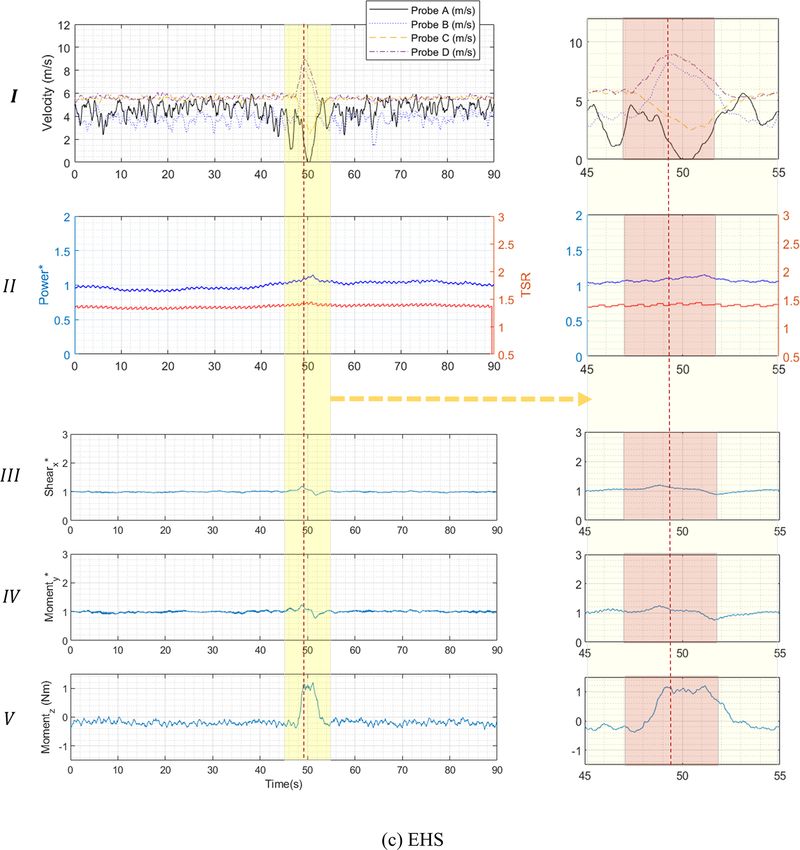
478 K. Shirzadeh et al.: Investigating the loads and performance of a model horizontal axis wind turbine
ditions in the IEC 61400-1 document (IEC, 2005) followed grids. While some of these studies produced various transient
by statistical analysis introduced in the latest edition (IEC, flows, none had attempted to reproduce the EOG and EWS
2019). Herein the power generation and loads on a scaled as per IEC standards and apply them to a wind turbine with a
HAWT are being tested under representative deterministic relevant scaling, which constitutes the main objective of the
gust design conditions as per IEC 2005. This is an extension present study. The work has been performed at the WindEEE
to the previous study (Shirzadeh et al., 2020) that incorpo- Dome at Western University Canada. Along with the numer-
rated the developments of the corresponding scaled extreme ical simulations and field data, this setup can contribute to
operational gust (EOG) and extreme wind shears (EWSs) and fast development of the new control prototypes of HAWT
included the extreme vertical and horizontal shears (EVSs for customized transient wind effects.
and EHSs), in the WindEEE Dome. The paper is organized as follows. Section 2 briefly
From an aerodynamic perspective the effective angle of at- presents the target deterministic operational extreme condi-
tack on the blades and consequently the global lift and drag tions. Section 3 details the WindEEE chamber and the ex-
forces increase during wind gust conditions, which result in periment setups; this section also provides the details about
blade torque, thrust and root moment amplification. Several the uniform flow fields used as reference values for compar-
experimental studies have been conducted to control the rotor isons. Section 4 presents the results from EWSs and EOG
aerodynamics under these transient events. The application and the capability of the facility in reproducing these condi-
of the adaptive camber airfoil in a gusty inflow generated by tions. Section 5 is dedicated to conclusions.
are active grid was investigated by Wester et al. (2018). These
types of airfoils have coupled leading and trailing edge flaps,
2 Deterministic extreme operating conditions
which can be adjusted to de-camber the profile with increas-
ing lift force. This proved to reduce the integral lift force Prior to introducing the deterministic gust models, it is in-
about 20 % at the peak in a gust event. Petrović et al. (2019) formative to know how the standard (IEC, 2005) classifies
developed an algorithm for a PI controller of the pitch angles wind turbines based on a reference wind speed and turbu-
of a scaled wind turbine in the wind gust conditions gener- lence intensity (TI). The TI in the standard is given for a
ated by an active grid. Using the algorithm, they were able specific height and is defined as the ratio of the mean stan-
to reduce over-speeding of the rotor and the blades’ bending dard deviation of wind speed fluctuations to the mean wind
moments. speed value at that height, both calculated in 10 min inter-
The effect of the wind shears on wind turbine aerodynam- vals. Three classes of reference wind speeds (Uref : I–III)
ics has been studied by several investigators. The effect of and three classes of turbulence intensities (Iref : A–C) are de-
various steady shear flows and turbulence intensities, gener- fined, which gives a combination of nine external turbine de-
ated by active grid, on the near-wake region of a small-scale sign conditions that have specified values. One further class
turbine was investigated by Li et al. (2020) using particle for special conditions (e.g. off-shore and tropical storms) is
image velocimetry (PIV) measurements. It has been found considered which should be specified by the designer. Cor-
that the absolute mean velocity deficit in this region remains respondingly, extreme wind speed models as a function of
symmetric, and it is insensitive to the inflow non-uniformity. height (Z) with respect to the hub height (Zhub ) with recur-
Also, the mean power production does not change with the rence periods of 50 years (Ue50 ) and 1 year (Ue1 ) are defined
amount of the shear. However, the power fluctuation has a as follows:
linear correlation with the amount of background turbulence
intensity; in other words, the effect of higher shears trans- Z 0.11
lated as a higher inflow turbulence and therefore higher fluc- Ue50 (z) = 1.4Uref , (1)
Zhub
tuations in power. Similar results were reported by Sezer-
Ue1 (z) = 0.8Ue50 (z). (2)
Uzol and Uzol (2013), who used a three-dimensional un-
steady vortex-panel method to investigate the effect of tran-
Based on the turbulence class, the streamwise hub height ve-
sient EWS on the performance of a HAWT. They found that
locity standard deviation (σu ) is defined by what is called the
due to the EWS, the blades experience asymmetrical surface
normal turbulence model as Eq. (3).
pressure variations. Consequently, the rotor produces power
and thrust with a high amplitude of fluctuations, which can σu = Iref 0.75Uhub + 5.6
(3)
cause significant structural issues and reduce the lifetime of
the turbine. From the field data perspective, it has been re- Uhub is the average velocity at hub height.
ported that for the same reference wind speed, higher turbu- Based on Eqs. (2) and (3), the hub height gust magni-
lence intensities result in relatively higher-power efficiencies tude (Ugust ) is given as
below the nominal operational condition, but the efficiency
decreases in transition to rated power (Albers et al., 2007).
σu
Mostly, transient flow fields have been previously gen- Ugust = min 1.35 Ue1 − Uhub ; 3.3 . (4)
erated either numerically or physically by means of active
1 + 0.1 D 3u
Wind Energ. Sci., 6, 477–489, 2021 https://doi.org/10.5194/wes-6-477-2021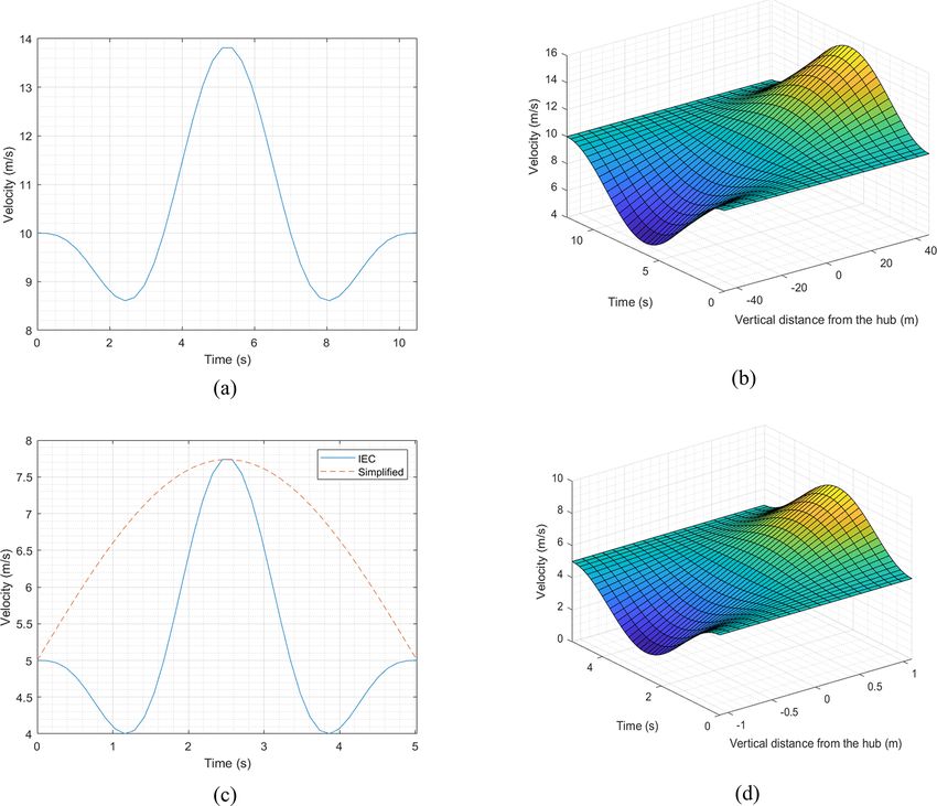
K. Shirzadeh et al.: Investigating the loads and performance of a model horizontal axis wind turbine                                 479

Figure 1. Extreme operational conditions for a full-scale HAWT IIIB class with 92 m diameter and hub height of 80 m at 10 m s−1 uniform
wind speed, (a) extreme operational gust and (b) extreme vertical shear on the rotor with hub height as reference, The scaled extreme
condition, (c) the IEC EOG and the simplified EOG that was targeted, and (d) extreme vertical shear. Adopted from Shirzadeh et al. (2020).

Figure 2. WindEEE dome, (a) the test chamber and the contraction walls with the flow recirculation path through the outer shell in closed-
circuit 2D flow mode, and (b) the adjustable vanes at the inlets of the 60 fans at 70 % opening vane state.

https://doi.org/10.5194/wes-6-477-2021                                                          Wind Energ. Sci., 6, 477–489, 2021
480 K. Shirzadeh et al.: Investigating the loads and performance of a model horizontal axis wind turbine
Taking t = 0 as the beginning of the gust, the velocity time and d. These are the inflow fields that are considered in the
evolution of the EOG is defined as present experiments. Therefore, based on this assumption,
the turbine should be working at 1.1 TSR. Also due to hard-
U (t) =
( ware limitation in the physical experiments, the EOG has
Uhub − 0.37Ugust sin 3π t
1 − cos 2π t
; when 0 ≤ t ≤ T , been simplified by excluding the velocity drops before and
T T (5)
Uhub ; when t > T or t < 0. after the main peak as is shown in Fig. 1c as the red dashed
line. This simplification stretches the actual rising and falling
T is the duration of the EOG, specified as 10.5 s, D is the time, yet this is the compromise that was made due to hard-
diameter of the rotor, and 3u is the longitudinal turbulence ware limitations. For a wind turbine that operates in a specific
scale parameter, which is a function of the hub height: average wind, it is the velocity excursion above the average
0.7Zhub for Zhub ≤ 60 m, wind speed that is important to capture. More detailed in-
3u = (6) formation about the scaling method and the extreme opera-
42 m for Zhub > 60 m.
tional condition (EOC) flow fields is accessible in Shirzadeh
The EWS can be added to or subtracted from the main uni- et al. (2020).
form or ABL inflows. The EVS velocity time evolution at a It is worth mentioning that these extreme operational con-
specific height (Z) can be calculated using Eq. (7). dition models are relatively simple and not able to capture the
real dynamics of the ABL flow field that directly affect the
UEVS (Z, t) = performance of the turbine (Schottler et al., 2017; Wächter et
al., 2012). However, they provide practical guidelines for the
0.25
Z−Zhub D 2πt
D 2.5 + 1.28σu 3u 1 − cos T ; when 0 ≤ t ≤ T , (7)
0; when t > T or t < 0. development and wind tunnel testing of HAWTs.
The EWS duration is 12 s. For a commercial IIIB class
3 Experimental methodology
HAWT with 92 m diameter and 80 m tower hub height, at
10 m s−1 average velocity, the prescribed EOG and EVS are As mentioned earlier, in this study similar inflow fields with
presented in Fig. 1a and b. The time windows in these figures the ones developed in Shirzadeh et al. (2020) were repro-
start and end with the extreme event. The standard gust du- duced to investigate the responses of the wind turbine to
rations in operation conditions are relatively long compared these scaled transient conditions. For each extreme event
to the response time of scaled wind turbines. Herein, we as- only one measurement run was performed. The reproducibil-
sume these time durations (10.5 s for EOG and 12 s for EWS) ity of these events was ensured by direct comparison with the
correspond to four complete rotor revolutions in commercial previous study.
wind turbines, which typically have a rotational speed in the
range of ∼ 15–20 RPM. In other words, the gust time dura-
3.1 WindEEE Dome
tion is equal to the advection of the four complete tip vortex
loops from a specific blade in the wake by the free stream. The experiments were carried out at the Wind Engineering,
Accordingly, the timescale becomes a function of rotor an- Energy and Environment (WindEEE) Dome at Western Uni-
gular velocity or the tip speed ratio (i.e. TSR, the ratio of the versity, Canada. The test chamber has a 25 m diameter foot-
blade tip linear velocity over the free stream), free stream ve- print and 3.8 m height with a total number of 106 fans, of
locity and diameter of the rotor; for a scaled wind turbine, the which 60 fans are mounted along one of the hexagonal walls
duration corresponding to four revolutions in similar nominal in a 4 × 15 matrix and 40 fans are mounted on the rest of
operating conditions is on the order of 1 s. The experiments the peripheral five walls (Fig. 2a). Six other larger fans are
in the earlier study showed that the fastest possible gust ob- in a plenum above the test chamber, usually being used for
tained in the WindEEE Dome with the desired peak factor 3D flows like tornadoes and down bursts (Hangan et al.,
was around 5 s (Shirzadeh et al., 2020). Therefore, it is pos- 2017). In the present study, experiments were carried out us-
sible to relevantly decrease the wind speed and TSR to match ing the dome in 2D flow (e.g. ABL, uniform straight flows)
up the parameters based on the assumption above that results closed-circuit mode in which just the 60-fan wall is operated.
in Eq. (8): In this mode the flow recirculates from the top through the
Ts Uhub λ outer shell as is shown in Fig. 2a. Each of these fans are 0.8 m
= 4, (8) in diameter and are individually controlled to a percentage
πD of their 30 kW maximum power using variable frequency
where Ts is the scaled time (here it is 5 s) and λ is the oper- drives. In order to reach higher velocities at lower fan power
ating TSR. Assuming a similar IIIB class HAWT with a hub set points at the test chamber for generating EOG, a 2D con-
height of ∼ 2 m with the 2.2 m diameter-scaled wind turbine, traction with ratio of 3 was installed at the outlet of the 60-
at 5 m s−1 average hub height velocity, the extreme condi- fan wall that extends for 7.5 m downstream (Fig. 2a). These
tion profiles look identical to the full-scale ones (the same fans are equipped with adjustable inlet guiding vanes (IGVs).
peak factor but different gust time) as presented in Fig. 1c They can be adjusted stationarily from 0 % open (close) to
Wind Energ. Sci., 6, 477–489, 2021 https://doi.org/10.5194/wes-6-477-2021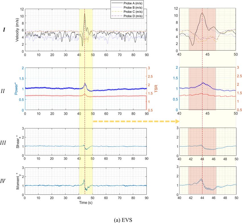
K. Shirzadeh et al.: Investigating the loads and performance of a model horizontal axis wind turbine 481
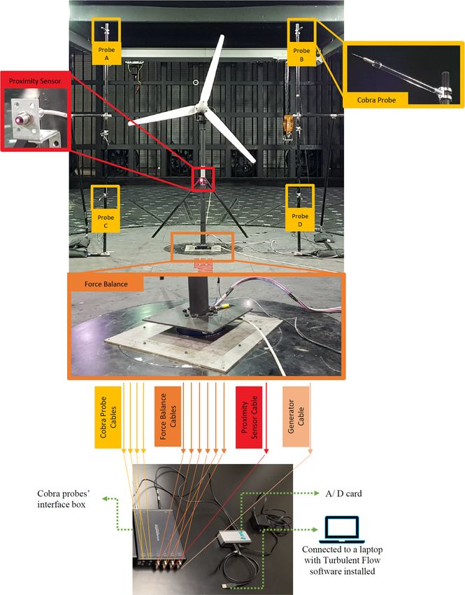
Figure 3. Setup for measuring power performance and dynamic loads for different types of inflow.
100 % open or dynamically in an open–close cycle (Fig. 2b). bine rotor plane. More specific details about cobra probes
By using this feature the EOGs were produced. The EWSs are found in Shirzadeh et al. (2020). The wind turbine was
were produced by power modification of the five middle fan mounted on a six-component force balance sensor for mea-
columns (20 fans). Therefore, contraction walls had no effect suring all three shear forces and three moments at the base
on the EWS flow fields. of the tower. In addition, a light photoelectric diffuse reflec-
tion proximity sensor (Autonics BR200-DDTN) was used,
3.2 Experimental setup for power and load performance which gives a voltage pulse once it detects a light reflection
from the blade passing in front. Using the pulse, one can
To measure the velocity of the flow field, four cobra probes measure the angular velocity of the rotor with a high reso-
(TFI Ltd., 2011) are used in a plane 1 m upstream (∼ 0.5 D) lution (three times a revolution). The turbine has 1 kW rated
of the rotor with 1.3 m left and right offset from the rotor’s power at 12 m s−1 wind speed and a nominal TSR of 5; de-
hub. The probes are set at 3 m and 0.8 m heights correspond- tailed specifications of blade geometry and the power curve
ing to the highest and lowest heights of the rotating blades’ of the turbine are available in Refan and Hangan (2012). This
tips (Fig. 3). With this configuration the cobra probes can wind turbine is equipped with a three-phase AC generator. A
give a proper perception of the flow field over the wind tur-
https://doi.org/10.5194/wes-6-477-2021 Wind Energ. Sci., 6, 477–489, 2021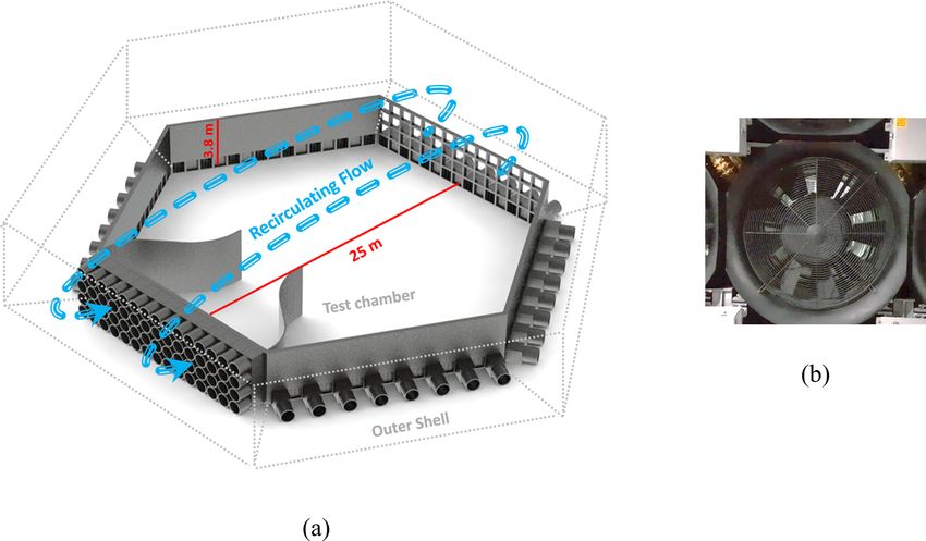
482 K. Shirzadeh et al.: Investigating the loads and performance of a model horizontal axis wind turbine
Figure 4. The arrangement of cobra probes and HAWT relative to
the local coordinate system.
Figure 5. Comparison of turbulent velocity spectra for the 5 m s−1
uniform flow cases.
specific electrical circuit was used to convert the voltage and
current to DC and feed the power to the resistors. The last
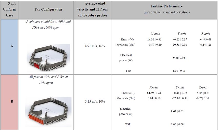
parameter that was monitored was the voltage from the ter- wind inflow cases (cases A and B in Table 1). Cases A and B
minals of the power resistors which were set at a constant were used to normalize the EWSs and the EOG respectively.
8.1 in order to keep the rotor at the desired TSR (1.1) that The reason for using different uniform cases is due to the
has been calculated based on the averaged wind speed from difference in the flow characteristics (TI and spectra) related
all the cobra probes. At the end, eight analogue voltage ca- to the different fan setups for each case. At this low TSR,
bles (six voltages from force balance, one from proximity considerable parts of the blades are in stall, and the TI mag-
sensor and one from load terminals) plus four cobra probe nitude can affect the flow behaviour on the suction side of the
cables gathered to one deck were synchronized and logged blades and result in noticeable difference in loads and power
at 2000 Hz frequency for 90 s for each experiment run. All performance of the wind turbine. The mean and rms values of
the signals were calibrated as zero in the turbulent flow data the data obtained from the force balance, turbine power and
acquisition software when the 60 fans were off. TSR from these two uniform cases are tabulated in Table 1.
The schematic of the positioning of the wind turbine and The bolded values in this table will be used to normalize the
the cobra probes relative to the local coordinate system (cen- corresponding data from the transient experiment cases.
tre of the WindEEE dome/base of the tower) is depicted in The spatially averaged turbulence spectra by the four cobra
Fig. 4. Some of the loads at the base are inherently correlated probes for these two uniform cases are presented in Fig. 5.
with the performance of the wind turbine. Based on this lo- There is a consistent noise from the fans with its harmon-
cal coordinate system, the most important force in terms of ics at some specific high frequencies (∼ 200 and 400 Hz in
both magnitude and correlation with turbine performance at case A, ∼ 200 and 600 Hz in case B). Due to the steadi-
the base is in the X direction, which represents the thrust of ness of the flow, a large share of the energy is distributed
the rotor, plus the drag force of the tower. The X moment at the low-end frequencies (i.e. frequencies lower than 3 Hz).
represents torque on the generator plus induced vortex shed- In this region, the two cases show the same energy distri-
ding moment; the Y moment shows the bending moment due bution. However, for frequencies higher than and equal to
to drag on the whole structure (correlated to the forces in the 3 Hz or length scales of 1.65 m and smaller (based on the
X direction). The moment around the Z axis shows the twist frozen turbulence hypothesis at 5 m s−1 average wind speed,
due to horizontal non-uniformity of the flow. The Z force 1 −1 = 1.65 [m]), the difference in energy distribu-
3 Hz × 5 m s
represents the lift on the structure. tion is noticeable with lower turbulence energy in case B
in all the corresponding frequencies relative to case A. All
3.3 Baseline uniform inflows the spectra follow the −5/3 slope consistent with the Kol-
mogorov theory in the inertial subrange (Pope, 2000).
As mentioned earlier, in this study four unsteady extreme
condition cases (EVS, EHS, negative EVS and EOG) are
3.4 Uncertainty analysis
considered for the investigation. For the EWSs just the
20 middle fans and in the EOG all of the fans were operated. The epistemic uncertainty of the cobra probes depends on
Some of the results from power performance and loadings of turbulence levels, but is generally within ±0.5 m s−1 up to
each case are normalized with their corresponding averaged about 30 % turbulence intensity according to the manufac-
data from one of the two different 5 m s−1 steady uniform turer (TFI Ltd., 2011). Considering the 5 m s−1 average wind
Wind Energ. Sci., 6, 477–489, 2021 https://doi.org/10.5194/wes-6-477-2021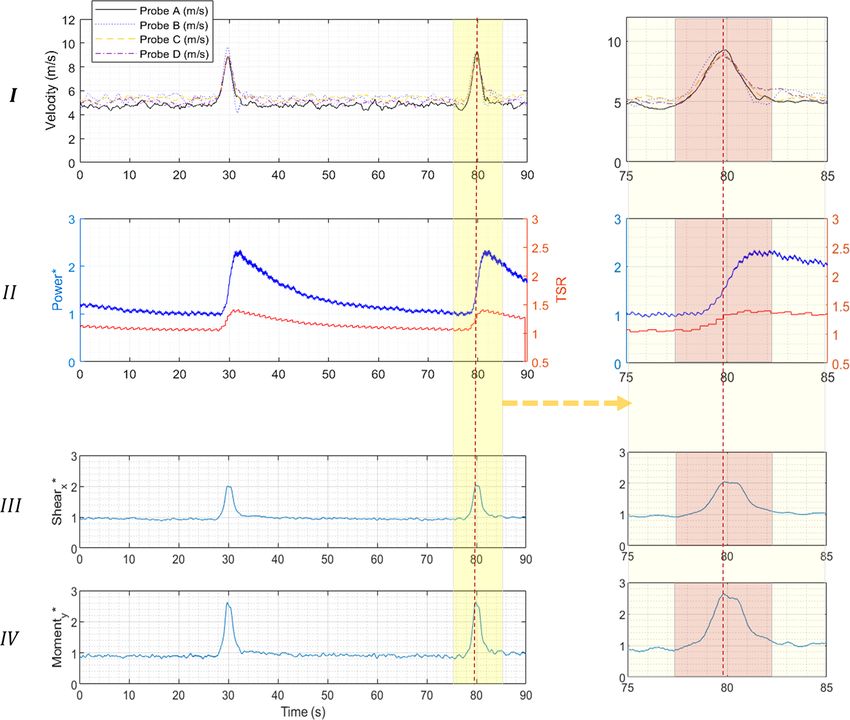
K. Shirzadeh et al.: Investigating the loads and performance of a model horizontal axis wind turbine                            483

Table 1. The mean values of loads and power generation in different steady uniform cases (with the same load, 8.1 ).

Table 2. Nominal accuracy for the JR3 (75E20S4-6000N) in each axis based on the data sheet.

            Nominal     X axis                             Y axis                             Z axis
            accuracy
            Force       ±0.25 % × 6000 N = ±15 N           ±0.25 % × 6000 N = ±15 N           ±0.25 % × 12 000 N = ±30 N
            Moment      ±0.25 % × 1100 N = ±2.75 Nm        ±0.25 % × 1100 N = ±2.75 Nm        ±0.25 % × 1100 N = ±2.75 Nm

velocity in the experiments, the uncertainty of the probes is          is too small (7 cm diameter), which made the mounting pro-
10 %. The JR3 multi-axis force and torque sensor (75E20S4-             cess very challenging, with the possibility of damaging the
6000N) at the base of the tower has a stated ±0.25 % nomi-             sensor. Only the X (thrust-aligned) force and Y (overturn-
nal accuracy based on the maximum rated load for each axis;            ing/nodding) moment will be presented in the Results sec-
refer to Fig. 4 for the axis orientation relative to the wind          tion, as the other loads have very small mean values leading
tunnel. The nominal accuracy of this sensor along each axis            to unacceptably high uncertainties.
based on the data sheet is tabulated in Table 2. These val-               All the values from the measuring instruments presented
ues represent the largest possible uncertainties that the sen-         in Sect. 4 have been filtered by the moving-average method
sor might have; however, generally, it is more precise. A              except for the rotor speed. The averaging windows for the
special calibration process was performed by the JR3 com-              wind velocities, the generator voltage and the loads were
pany per request, using 58.75 Nm (400 lb · 6.5 in) reversed            chosen as 0.2, 0.2 and 0.5 s respectively based on the cri-
and repeated moments about the Y axis; the reported val-               teria described in Chowdhury et al. (2018), which preserved
ues were 58.77, −58.63, 58.86 and −58.98 Nm. This calibra-             the main shape of signal time history, filtering low-powered
tion test implies a ±0.12 Nm error on average when loaded              high-frequency fluctuations. Therefore, the processed data
close to the range of our experiments. This load sensor has            have aleatoric or random uncertainties within. The combined
a 19 cm diameter, which made mounting the turbine directly             uncertainties have then been calculated with the root sum
on its surface possible. It would have been ideal to use the           squared of these two types of uncertainties and presented as
JR3 (30E12A4-40N) model; however, the size of this model               the percentage of their corresponding mean values in Table 3.

https://doi.org/10.5194/wes-6-477-2021                                                          Wind Energ. Sci., 6, 477–489, 2021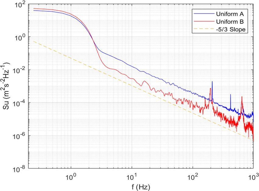
484 K. Shirzadeh et al.: Investigating the loads and performance of a model horizontal axis wind turbine
Figure 6.
In this table, the epistemic uncertainty for the Y moment has Table 3. The combined uncertainty estimation of the measured val-
been calculated based on the calibration results, but value for ues averaged in all the experiments.
the X force is based on the data sheet. As mentioned earlier,
the X force and the Y moment are caused by the rotor thrust Mean Epistemic Aleatoric Combined
values uncertainty uncertainty uncertainty
and drag. Therefore, having high uncertainty in the X force
can be compensated for by comparing it to the Y moment, Wind velocity 5 m s−1 ±10 % ±9.60 % ±13.86 %
which has a more reliable value. The propagation of uncer- Power 0.70 W ∼ ±0 % ±5.71 % ±5.71 %
X force 14.37 N ±104.38 % ±7.86 % ±104.66 %
tainty due to normalizing some of the parameters in extreme Y moment 23.00 Nm ±0.52 % ±13.78 % ±13.78 %
operational cases with steady cases has been neglected.
4 Test case results
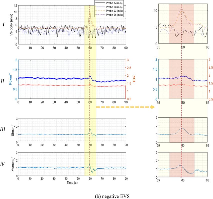
arranged as follows: window I shows the filtered wind ve-
4.1 Unsteady EWS locity time histories from the four cobra probes, window II
shows the normalized electrical power along with the TSR,
The time history of the results from EVS, negative EVS and and windows III and IV show the filtered force and moment
EHS cases generated by changing the fan power set points time histories exerted at the tower base in the X direction and
is presented in Fig. 6a–c respectively. There are four win- around the Y axis respectively. Note that in these figures, the
dows (I, II, III and IV) in all of these panels which have been axis force has been referred as shear, as it exerts a shear force
Wind Energ. Sci., 6, 477–489, 2021 https://doi.org/10.5194/wes-6-477-2021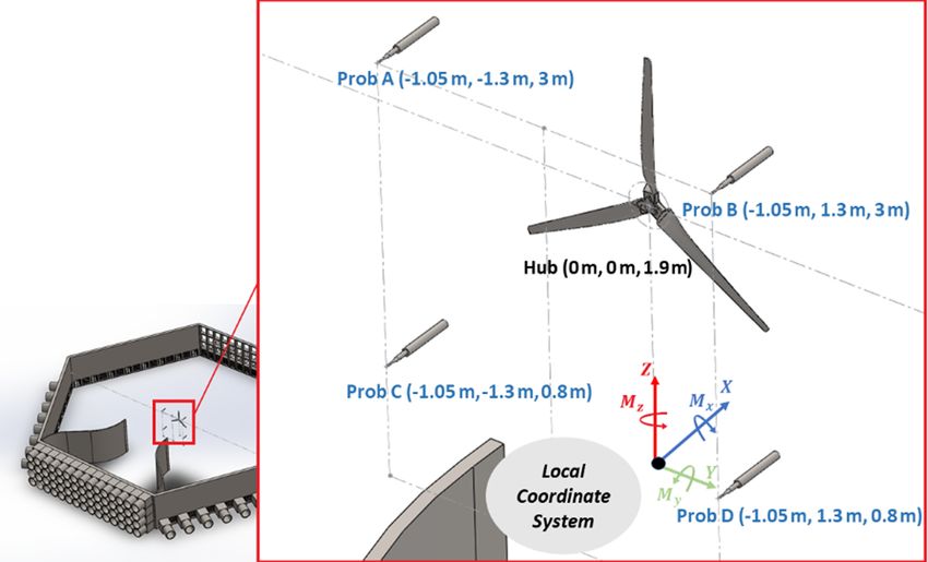
K. Shirzadeh et al.: Investigating the loads and performance of a model horizontal axis wind turbine                        485

Figure 6.

at the base. The starred axis indexes are normalized by their      Shirzadeh et al. (2020). The EVSs do not have any signifi-
corresponding values from the uniform case A. In addition,         cant effect on the loads at the base of the tower (windows III
a 10 s window around the extreme events has been 4× mag-           and IV in Fig. 6a and b).
nified and replotted at the right sides of these panels which         The highly correlated behaviour between force on the
present the effect of extreme events in better details. The ver-   X axis and moment around the Y axis is clear in all these
tical red dashed line passes through the first wind velocity       figures, comparing windows III and IV.
peak, and it has been assumed as the centre of the event.             In the EHS case, the most important load component at
Based on this line a 5 s red window has been depicted that         the tower base in terms of magnitude and its correlation with
highlights the theoretical duration of the extreme event in the    the extreme event is the Z-axis moment. Therefore, the addi-
magnified plots.                                                   tional window V in Fig. 6c shows this extreme condition in-
   Window II in all figures illustrates that these transient       duces a 1.2 Nm yaw moment on the structure. While the high
shear cases do not have a significant effect on the overall        probable uncertainty in reporting this value based on Table 2
power performance of the wind turbine. The initial increase        has been recognized, if one normalizes this number using
and decrease in power productions are just due to the time lag     Eq. (9), one gets 0.009414. Accordingly, for a full-scale wind
between the high and the low peaks of the shears (∼ 1.5 s)         turbine with 92 m diameter working in an average 10 m s−1
reaching the rotor, which is noticeable from the magnified         wind speed, the induced yaw moment on the structure by an
cobra probe time history in window I in Fig. 6a–c. More de-        EHS event would be 351 kNm.
tails about the extreme event velocity fields are accessible in

https://doi.org/10.5194/wes-6-477-2021                                                    Wind Energ. Sci., 6, 477–489, 2021
486                      K. Shirzadeh et al.: Investigating the loads and performance of a model horizontal axis wind turbine

Figure 6. The time history of the results from all the measuring instruments in (a) the EVS and (b) the negative EVS. Windows I, II, III
and IV from top to bottom in each panel show the wind velocities from four cobra probes, the power performance of the turbine, the X shear
and the Y moment at the base of the tower respectively. Panel (c) is for the EHS and has an additional window V that reports the Z moment.
The starred axis indexes are normalized by their corresponding value from uniform case A. The 10 s window around the extreme events has
been magnified and replotted at the right side of each panel with a red 5 s window highlighting the theoretical duration of the extreme event
and the red dashed line assumed as the centre of the events which passes through the first velocity peak.

                                                                         2016). Accordingly, the amount of yaw moment induced by
             Mz                                                          the EHS (varying between 0 and 350 kNm) is at least 3 times
CMz =    1
                     ,                                          (9)
             2                                                           the magnitude of the yaw experienced by the turbine in uni-
         2 ρU AD
                                                                         form inflow conditions.
where ρ is the density of the air, A is the swept area of the
rotor and D is the diameter. As a full-scale (87 m diameter)
                                                                         4.2   Unsteady EOG
numerical simulation under steady velocity of 10 m s−1 with
typical yaw condition suggests, the yaw moment can vary                  The EOG significantly affected the power generation and the
between ∼ 30 and 90 kNm as the blades rotate (Cai et al.,                loads. As the window II in Fig. 7 shows, this event can dan-

Wind Energ. Sci., 6, 477–489, 2021                                                            https://doi.org/10.5194/wes-6-477-2021
K. Shirzadeh et al.: Investigating the loads and performance of a model horizontal axis wind turbine 487 Figure 7. The time history of the results from all the probes in EOG using IGVs: window I shows the wind velocities from four cobra probes, window II shows power performance of the turbine, and windows III and IV show the X shear and Y moment at the tower base. The starred axis indexes are normalized by their corresponding value from uniform case B. The 10 s window around the extreme events has been magnified and replotted at the right side with a red 5 s window highlighting the theoretical duration of the extreme event and the red dashed line assumed as the centre of the events which passes through the velocity peaks. gerously increase the rotor rotational speed without control terwards (window II). The extractable energy in a gust with a systems (the TSR increased 33 %). The electrical power in- specific amplitude and time duration partially accumulates in creased 148 % at the end of the gust event. However, the elec- the rotor rotational momentum with the excess in the form of trical power generation might not be the proper quantity for higher instantaneous power generation. After the gust event, comparison at these low rotational speeds. The generator ef- the stored momentum gradually transforms into power. ficiency is highly dependent on the rotor speed. Therefore, some part of this boost in power production is due to the fact that generator efficiency also increased as the rotor speeded 4.3 Reproducibility of the extreme events up. The mechanical power should be a better quantity for In order to investigate the reproducibility of these extreme comparison, but it was not possible to measure with the cur- events in the WindEEE dome, a normalized cross correlation rent setup. The overall drag on the structure (X shear) and of the velocity signals between the current and the previous its bending moment (Y moment) at the base increased by study (Shirzadeh et al., 2020) has been performed. The refer- 105 % and 167 % respectively. According to the magnified ence probes from the previous study are probes H and B that windows in Fig. 7, the loads have a similar profile shape as were installed at similar heights or lateral distances depend- the gust with the same order of rising and falling time (win- ing on the event. For example, probe H in the EVS event dows III and IV). However, the power generation peak hap- was located at 3 m height in the previous study, similar to pens at the end of the gust event and then slowly decays af- probes A and B in this study. For the analysis, firstly, the https://doi.org/10.5194/wes-6-477-2021 Wind Energ. Sci., 6, 477–489, 2021
488                      K. Shirzadeh et al.: Investigating the loads and performance of a model horizontal axis wind turbine

Table 4. The reproducibility analysis based on probes H and B from       The unsteady EVSs and EHS did not have any noticeable
the previous study (Shirzadeh et al., 2020).                          effect on the power performance and overall loading at the
                                                                      base of the turbine. Nevertheless, EHS induced a significant
    Extreme        Reference         Normalized           Overall     yaw moment on the structure. These extreme shears could
    event           probe          cross correlation     similarity   induce severe fatigue loads at the blade bearings, blade roots
                    Probe H      Probe A       Probe B                and yaw bearing. Having load cells at the blade roots and
                                 91.89 %       93.19 %                nacelle–tower junction or yaw bearing could have given more
    EVS                                                  94.33 %
                                                                      information about the load dynamics and the out-of-plane
                    Probe B      Probe C       Probe D
                                                                      moment in these scenarios.
                                 95.75 %       96.52 %
                                                                         The EOG affects the turbine significantly. Results showed
                    Probe H      Probe A       Probe B                that the power generation and loadings can increase signif-
                                 94.49 %       90.52 %                icantly with a high dynamic behaviour. In the EOG event,
    Negative EVS                                         95.10 %
                    Probe B      Probe C       Probe D                the loading profiles are correlated with the shape of the gust
                                 97.65 %       97.77 %                event itself (the peak of the loads are at the same point as the
                                                                      gust peak), but the power generation’s peak happens at the
                    Probe H      Probe B       Probe D
                                                                      end of the gust event.
                                 96.48 %       98.47 %
    EHS                                                  97.61 %         Overall, this study presents an alternative experimental
                    Probe B      Probe A       Probe C                procedure for investigating the global loading and power
                                 96.32 %       99.18 %                generation of a wind turbine under scaled reproducible de-
                    Probe H      Probe A       Probe B                terministic transient wind conditions. The procedure has the
                                 99.29 %       98.72 %                potential to be improved upon and used for developing and
    EOG                                                  99.17 %
                                                                      testing new wind energy prototypes in transient conditions.
                    Probe B      Probe C       Probe D
                                 99.26 %       99.43 %
                                                                         In future work, for the EVS and EHS cases it is advisable
                                                                      to investigate the loads on the blade roots and bearings as
                                                                      well as yaw bearing to implement a fatigue load analysis. In
                                                                      the present study the TSR was determined from wake effect
velocity data in a 20 s window around the event have been             scaling and physical limits of the test apparatus, resulting in a
extracted from both velocity time histories. Secondly, with a         TSR ∼ 1.1. In future work, an attempt should be made to test
specific amount of time lag between the velocity signals from         at higher TSR through test apparatus and controller modifi-
this study and the reference probe, the extreme events were           cations. Testing of the effect of different extreme event du-
perfectly aligned. Finally, the normalized cross correlation          rations at different operating TSRs would help validate the
was calculated. This way, the shapes of the velocity signals          suggested time scaling.
were compared. At the end, the averaged value of similarity
from all four probes has been reported as the overall similar-
ity of these events to the previous study as it has been tab-         Code availability. Code is available upon request.
ulated in Table 4. Accordingly, the IGVs are highly capable
of generating similar profiles of EOG with more than 99 %
of similarities. Modulating the fan power set points for creat-       Data availability. Data are available upon request.
ing the EHS and EVSs shows consistent results, with around
97 % and 94 % similarities.
                                                                      Supplement. The supplement related to this article is available
5     Conclusions                                                     online at: https://doi.org/10.5194/wes-6-477-2021-supplement.

An experimental study has been carried out to investigate
the effect of transient extreme operating conditions based on         Author contributions. KS carried out all the experiments with
the IEC standard (specifically EWSs and EOG) tailored and             supervision of HH. KS wrote the main body of the paper with input
scaled for a 2.2 m diameter HAWT at the WindEEE dome at               from all authors.
Western University. The main assumption used for the length
and time scaling is that the duration of each extreme condi-
                                                                      Competing interests. The authors declare that they have no con-
tion is equal to the advection time of the four tip vortex loops
                                                                      flict of interest.
in the wake by the free stream. Other parameters were ad-
justed accordingly to accommodate for hardware limitations
in generating the flow fields. Two uniform cases as the base-         Acknowledgements. All authors thank Gerald Dafoe and Tris-
lines for comparing the effect of different scenarios were also       tan Cormier for helping with the measurement setups, with special
carried out.                                                          thanks to George Sakona for calibration of the load sensor. The

Wind Energ. Sci., 6, 477–489, 2021                                                         https://doi.org/10.5194/wes-6-477-2021
K. Shirzadeh et al.: Investigating the loads and performance of a model horizontal axis wind turbine 489
present work is supported by the WindEEE dome CFI grant and Li, L., Hearst, R. J., Ferreira, M. A., and Ganapathisubra-
by NSERC Discovery Grant R2811A03. mani, B.: The near-field of a lab-scale wind turbine in tai-
lored turbulent shear flows, Renew. Energy, 149, 735–748,
https://doi.org/10.1016/j.renene.2019.12.049, 2020.
Financial support. The
present work is supported by Milan, P., Wächter, M., and Peinke, J.: Turbulent Char-
the WindEEE dome CFI grant and by NSERC Discovery acter of Wind Energy, Phys. Rev. Lett., 110, 138701,
Grant R2811A03. https://doi.org/10.1103/PhysRevLett.110.138701, 2013.
Petrović, V., Berger, F., Neuhaus, L., Hölling, M., and Kühn,
M.: Wind tunnel setup for experimental validation of
Review statement. This paper was edited by Alessandro Bian- wind turbine control concepts under tailor-made repro-
chini and reviewed by Rodrigo Soto and one anonymous referee. ducible wind conditions, J. Phys.: Conf. Ser., 1222, 012013,
https://doi.org/10.1088/1742-6596/1222/1/012013, 2019.
Pope, S. B.: Turbulent scalar mixing processes, Cambridge Univer-
sity Press, Cambridge, 2000.
References Refan, M. and Hangan, H.: Aerodynamic Performance of a Small
Horizontal Axis Wind Turbine, J. Solar Energ. Eng., 134,
Albers, A., Jakobi, T., Rohden, R., and Stoltenjohannes, J.: In- 021013, https://doi.org/10.1115/1.4005751, 2012.
fluence of meteorological variables on measured wind turbine Rezaeiha, A., Pereira, R., and Kotsonis, M.: Fluctuations of angle
power curves, in: European Wind Energy Conference and Exhi- of attack and lift coefficient and the resultant fatigue loads for a
bition 2007, vol. 3., EWEC 2007, May 2007, Milan, Italy, 2007. large Horizontal Axis Wind turbine, Renew. Energy, 114, 904–
Anvari, M., Lohmann, G., Wächter, M., Milan, P., Lorenz, E., 916, https://doi.org/10.1016/j.renene.2017.07.101, 2017.
Heinemann, D., Tabar, M. R. R., and Peinke, J.: Short term fluc- Schottler, J., Reinke, N., Hölling, A., Whale, J., Peinke, J., and
tuations of wind and solar power systems, New J. Phys., 18, Hölling, M.: On the impact of non-Gaussian wind statistics on
063027, https://doi.org/10.1088/1367-2630/18/6/063027, 2016. wind turbines – an experimental approach, Wind Energ. Sci., 2,
Bossanyi, E. A., Kumar, A., and Hugues-Salas, O.: Wind 1–13, https://doi.org/10.5194/wes-2-1-2017, 2017.
turbine control applications of turbine-mounted LIDAR, J. Sezer-Uzol, N. and Uzol, O.: Effect of steady and transient
Phys.: Conf. Ser., 555, 012011, https://doi.org/10.1088/1742- wind shear on the wake structure and performance of a
6596/555/1/012011, 2014. horizontal axis wind turbine rotor, Wind Energy, 16, 1–17,
Burton, T., Jenkins, N., Sharpe, D., and Bossanyi, E.: Wind Energy https://doi.org/10.1002/we.514, 2013.
Handbook, 2nd Edn., John Wiley and Sons Ltd, Chichester, UK., Shirzadeh, K., Hangan, H., and Crawford, C.: Experimental and
2011. numerical simulation of extreme operational conditions for hor-
Cai, X., Gu, R., Pan, P., and Zhu, J.: Unsteady aerodynamics izontal axis wind turbines based on the IEC standard, Wind
simulation of a full-scale horizontal axis wind turbine using Energ. Sci., 5, 1755–1770, https://doi.org/10.5194/wes-5-1755-
CFD methodology, Energy Convers. Manage., 112, 146–156, 2020, 2020.
https://doi.org/10.1016/j.enconman.2015.12.084, 2016. TFI Ltd.: Cobra Probe, Turbulent Flow Instrumentation Pty
Chowdhury, J., Chowdhury, J., Parvu, D., Karami, M., and Hangan, Ltd, available at: https://www.turbulentflow.com.au/Products/
H.: Wind flow characteristics of a model downburst, in: Fluids CobraProbe/CobraProbe.php (last access: 12 June 2020), 2011.
Engineering Division Summer Meeting, 51555, V001T03A005, Tran, T. T. D. and Smith, A. D.: Incorporating performance-based
2018. global sensitivity and uncertainty analysis into LCOE calcula-
Feng, Y., Qiu, Y., Crabtree, C. J., Long, H., and Tavner, P. J.: tions for emerging renewable energy technologies, Appl. Energy,
Monitoring wind turbine gearboxes, Wind Energy, 16, 728–740, 216, 157–171, https://doi.org/10.1016/j.apenergy.2018.02.024,
https://doi.org/10.1002/we.1521, 2013. 2018.
Hangan, H., Refan, M., Jubayer, C., Romanic, D., Parvu, D., Wächter, M., Heißelmann, H., Hölling, M., Morales, A., Milan,
LoTufo, J., and Costache, A.: Novel techniques in wind en- P., Mücke, T., Peinke, J., Reinke, N., and Rinn, P.: The turbu-
gineering, J. Wind Eng. Indust. Aerodynam., 171, 12–33, lent nature of the atmospheric boundary layer and its impact
https://doi.org/10.1016/j.jweia.2017.09.010, 2017. on the wind energy conversion process, J. Turbulence, 13, N26,
IEC – International Electrotechnical Commission: IEC 61400-1: https://doi.org/10.1080/14685248.2012.696118, 2012.
Wind turbines – Part 1: Design requirements, 3rd Edn., Geneva, Wester, T. T. B., Kampers, G., Gülker, G., Peinke, J., Cordes, U.,
Switzerland, 2005. Tropea, C., and Hölling, M.: High speed PIV measurements of
IEC – International Electrotechnical Commission: IEC 61400-1: an adaptive camber airfoil under highly gusty inflow conditions,
Wind energy generation systems – Part 1: Design requirements, J. Phys.: Conf. Ser., 1037, 072007, https://doi.org/10.1088/1742-
4th Edn., Geneva, Switzerland, 2019. 6596/1037/7/072007, 2018.
https://doi.org/10.5194/wes-6-477-2021 Wind Energ. Sci., 6, 477–489, 2021You can also read