The 3D Spatial Autocorrelation of the Branching Fractal Vasculature - MDPI
←
→
Page content transcription
If your browser does not render page correctly, please read the page content below
acoustics

Article
The 3D Spatial Autocorrelation of the Branching
Fractal Vasculature
Kevin J. Parker 1, * , Jonathan J. Carroll-Nellenback 2 and Ronald W. Wood 3
 1    Department of Electrical and Computer Engineering, University of Rochester, Rochester, NY 14627, USA
 2    Department of Physics and Astronomy, University of Rochester, Rochester, NY 14627, USA;
      johnathan.carroll@rochester.edu
 3    Department of Obstetrics and Gynecology, University of Rochester Medical Center, Rochester, NY 14642,
      USA; ronald_wood@urmc.rochester.edu
 *    Correspondence: kevin.parker@rochester.edu; Tel.: +1-585-275-3294

 Received: 26 February 2019; Accepted: 2 April 2019; Published: 9 April 2019

 Abstract: The fractal branching vasculature within soft tissues and the mathematical properties
 of the branching system influence a wide range of important phenomena from blood velocity to
 ultrasound backscatter. Among the mathematical descriptors of branching networks, the spatial
 autocorrelation function plays an important role in statistical measures of the tissue and of wave
 propagation through the tissue. However, there are open questions about analytic models of the
 3D autocorrelation function for the branching vasculature and few experimental validations for
 soft vascularized tissue. To address this, high resolution computed tomography scans of a highly
 vascularized placenta perfused with radiopaque contrast through the umbilical artery were examined.
 The spatial autocorrelation function was found to be consistent with a power law, which then, in
 theory, predicts the specific power law behavior of other related functions, including the backscatter
 of ultrasound.

 Keywords: scattering; backscatter; ultrasound; tissue; medical ultrasound; fractal vasculature;
 tissue characterization

1. Introduction
     In optics, electromagnetics, and acoustics, the behavior of waves within a weakly inhomogeneous
medium can be related to properties of the spatial correlation function, a statistical measure of the
spatial patterns or fluctuations within the material [1,2]. Both the forward propagating wave and
the waves scattered from the inhomogeneities have distributions that have been linked to the spatial
patterns of the inhomogeneities. For example, under the Born approximation and assumptions of
stationarity, a key integral formula relates the ensemble average measures of backscattered intensity
to the material’s spatial correlation function as a 3D Fourier transform operation. A specific case
emerges if we consider the parenchyma within organs such as the liver, prostate, or placenta to be the
reference media, while the long, cylindrical fluid-filled, fractal branching vessels serve as the weak
scattering sites.
     Under that hypothesis the fractal branching structure of the fluid-filled vasculature will play a
major role in determining the propagation of waves in highly vascularized tissues. However, there
are few reported experimental results in the literature that can answer the key question: What is
the 3D spatial autocorrelation function of a fractal branching vasculature network from normal soft
tissue organs? The question has high significance because the 3D spatial autocorrelation function of
these scattering sites drives the statistics of wave propagation, including the millions of ultrasound
scans each year derived from backscattered echoes. We address this question directly by applying

Acoustics 2019, 1, 369–381; doi:10.3390/acoustics1020020                       www.mdpi.com/journal/acoustics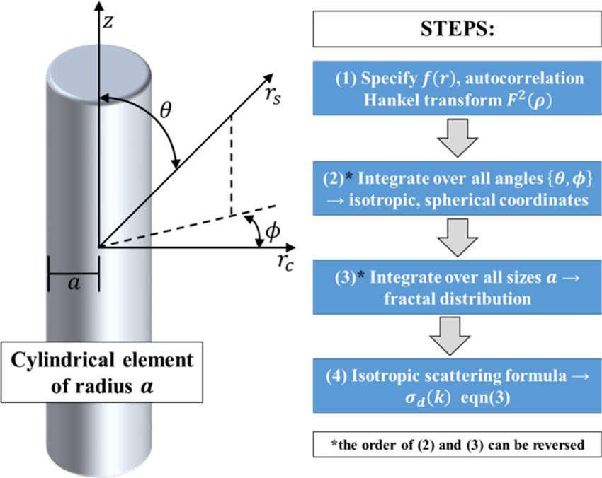
Acoustics 2019, 1                                                                                      370

radiopaque contrast to the vasculature system of a freshly delivered, intact placenta, obtaining high
resolution computed tomography (CT) scans, thresholding the 3D data set, and determining local
autocorrelation functions within interior regions. In theory, these results provide the quantitative link
between the properties of the fractal branching vasculature and physical measures such as scattering
and fluctuations in the forward propagating waves.

Fractal Structures and Scattering
     Since the popular work by Mandelbrot [3], the idea of self-similar structures occurring across
a wide range of scales has been applied to natural structures. The concept of fractals in biological
systems has seen numerous applications [4,5]. The nature of scattering from fractal structures has
also received attention, with the concept of a fractal dimension d f driving power law relations and
scattering behavior. For 3D space filling structures, the measured d f would be less than 3. Lin et al. [6]
modeled fractal aggregates and essentially argued that the long wavelength (low frequency or Rayleigh
scattering) limit would have the standard k4 dependence of backscatter where the wavenumber
k = ω/c, whereas the short wavelength (high frequency) limit would approach k(4−d f ) . Javanaud [7]
simply invoked a power law relation for scattering using d f as the scaling power.
     Shapiro [8] argued from a number of examples that a fractal structure would have a spectrum
(over some range of scales) that follows a power law, and derived a scattering formula for different
regimes under that assumption. One conclusion was that over some scale the backscattered intensity
would be proportional to k(4+ν) , where ν is a constant related to the fractal power law behavior.
Sheppard and Connolly [9] considered the optical scattering from random surfaces. Shear wave
scattering and loss were attributed to fractal structures in Lambert et al. [10] and Posnansky et al. [11].
The compatibility of these works requires further study.
     To summarize, the literature contains a number of theoretical functions in random media that
are related to fractals and are linked to different power law relations. However, we are left with some
open questions as to the particular autocorrelation function found in practice, and its implications for
wave propagation. These are addressed in the following sections.

2. Theory of Scattering Applied to Fractal Branching Networks

2.1. General Theory
     When considering scattering from random media, it can be shown [12–14] that the differential
scattering cross section per unit volume σd (k ) and the spatial correlation b(r̂ ) function of the
inhomogeneities are related by:
                                                      y
                                     σd (k) = k4 A           b(r̂ )e j2k̂·r̂ dVol,                     (1)

where k is the wavenumber, r̂ is the vector separation between two points within the ensemble average,
and A is a constant. Assuming the correlation function is isotropic and simply dependent on the
separation distance r, the volume integral reduces to:
                                                     Z ∞
                                                2π
                                    V I (k) =              r · b(r ) sin(2kr )dr,                      (2)
                                                 k   0

similar to the integral found in Equations (4), (9) and (11) from Parker [15], covering both acoustic and
electromagnetic scattering under the Born approximation.
     By comparing this to the form of the 3D Fourier transform in spherical coordinates with spherical
symmetry 3DS ={} [16,17], and shown in Appendix A, we may write:

                                      σd (k ) = A · k4 ·    3DS
                                                                  ={b(r ), k},                         (3)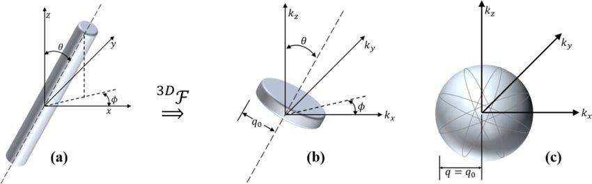
Acoustics 2019, 1                                                                                       371

                                 R∞
where 3DS ={b(r ), k } = (2π/k ) 0 r · b(r ) · sin(2kr )dr. Thus, the calculation of backscattering
reduces to the question of the 3D Fourier transform of the isotropic and spherically symmetric
ensemble-averaged correlation function of r. This spatial correlation function of cylindrical fluid-filled
vessels is considered next.

2.2. The Long Cylindrical Shape
     We considered fractal branching networks of the fluid-filled vasculature and other parallel fluid
channels to be comprised of long cylindrical sections, branching out in successive generations from
largest to finest.
     Assuming an isotropic spatial and angular distribution of each generation of fractal branching
structures, the goal was to average the autocorrelation function of a basic element across all angles
of incidence with respect to the propagating wave and across all size scales from very small
micro-channels of fluid to the largest arteries and veins that can exist within the organ. Specifically, we
will examine the fluid-filled cylinder of radius a:
                                                         (
                                                             κ0    r≤a
                                            f (r ) =
                                                             0     r>a                                  (4)
                                                          κ0 · a· J1 [2πa·ρ]
                                            F (ρ) =                 ρ

where κ0 is the fractional variation in density plus incompressibility, assumed to be  1 consistent with
the Born formulation, F (ρ) represents the Hankel transform, which is the two-dimensional Fourier
transform of a radially symmetric function, and ρ is the spatial frequency.
     First, assuming the fluid-filled cylinder is long in the z-axis, then the shape is one-dimensional
and its autocorrelation can be obtained from the inverse Hankel transform of the square of the shape’s
Hankel transform:
                                                   Z∞
                                  Bcyl (r ) = 2π        ρ · F (ρ)2 J0 (2πr · ρ)dρ,                      (5)
                                                   0

where ρ is the spatial frequency. Second, we assumed that cylinders of this kind exist within a fractal
geometry in an isotropic pattern. Therefore, copies of this were interrogated by the forward wave over
all possible angles. Thus, we formed a 3D isotropic correlation function for the shape by conversion to
spherical coordinates.
     Consider first, one infinitely long cylinder with a material property f (r)—symmetric—as shown
in Figure 1a and tilted at some arbitrary angle in a spherical coordinate system. It has a 3D transform
that is a thin disk (delta function kz but shown with finite thickness to make the graphic easier to
draw and visualize). Its transform is symmetric and given by the Hankel transform of order zero
F (ρ) = H{ f (r ), ρ}. A particular radius of value of q0 is shown for reference.
     Now, if we have an ensemble average of F2 (ρ) across many cylinders at random angles
(orientations) as shown in Figure 1a,b, but consider them as independent and uncorrelated (a cloud of
sparsely spaced scattering cylinders), then the ensemble average 3D transform is formed from the disk
function adding up over all realized angles. In the limit, any cylindrical radius q0 in Figure 1b forms a
spherical shell in the ensemble average (Figure 1c).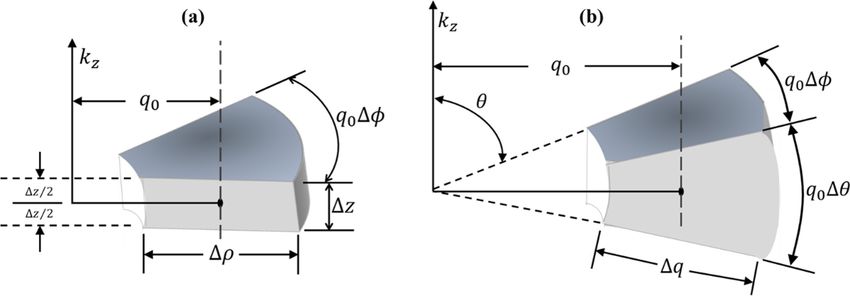
Now, if we have an ensemble average of F
2
(ρ) across many cylinders at random angles
(orientations) as shown in Figure 1a,b, but consider them as independent and uncorrelated (a cloud of
sparsely spaced scattering cylinders), then the ensemble average 3D transform is formed from the disk
function adding
Acoustics 2019, 1 up over all realized angles. In the limit, any cylindrical radius q0 in Figure 1b forms
372a
spherical shell in the ensemble average (Figure 1c).
Figure
Figure 1.
1. A
A cylindrical
cylindrical function
function (a) and its Hankel
Hankel transform
transform represented
representedin in3D
3DFourier
Fouriertransform
transformspace
space
(b).
(b). Rotations
Rotations around spherical coordinates similarly rotates
rotates the
the corresponding
corresponding transform,
transform,leading
leadingtotoaa
spherically
sphericallysymmetric
symmetricensemble
ensembleaverage
average(c).
(c).
Thus,
Acoustics 2019,the
Thus, ensemble
2 FOR
the average simply
PEER REVIEW
ensemble average simply takes
takes the
the Hankel
Hankeltransform functionF2F(ρ) ρfound
transformfunction found in Figure
in Figure5 1b
2
( )
andand
1b populates
populates thethespherically
sphericallysymmetric
symmetric 3D3D transformBs (Bqs )(,qshown
transform ) , shown in Figure 1c. 1c.
in Figure However,
However,there is ais
there
scaling of the cylindrical transform function
a scaling of the cylindrical transform function over the over the 2
(q)
spherical
F spherical ensemble
ensemble average. Specifically, the3D
average. Specifically, the 3D
spatial Fourier transform of the long cylinder B ( q ) = .
s oriented along the z-axis can be expressed as:
(8)
spatial Fourier transform of the long cylinder oriented along q the z − axis can be expressed as:
(xk,xk, we
FF2 2 k(3), z )
= =ℑ3DS
3 DS
{that:
b (={ r )}b
Thus, with reference to Equation yk,y k, zkconclude (r )}
=4 δ(3 DSk z )H0 {b(r ), ρ} (6)
σ d ( k ) = A ⋅=k δ⋅ (=k z δ)ℑ( {kzb0 ){(Fbr2)((,rρk))}, ρ } (6)
= δ (F k z2) Fk ( ρ )
2
4 ( )
where ρ2 = k2x + k2y , H0 {} is the Hankel transform = A ⋅ k of order zero [16], and δ(·) is the Dirac delta (9)
where ρ Next,
2 2 2
= k x + kthe 0 { disk
, thin } is(delta
the Hankel transform of k order coordinates
zero [16], and δ ( ⋅) is the
as FDirac
2 ( ρ ) δdelta
function. y function) in cylindrical represented 0 (k z )
F ( k ) , Bs (coordinates
3 2
must be converted
function. Next, the to a thin
thin diskdisk = coordinates
in spherical
(delta function) Ak
in cylindrical q0 )δ(θ − π/2 as F in( ρFigure
) as considered
represented
2
) δ ( k2,)
0 z
where the common radius ρ0 =2 q0 and ∆ρ = ∆q. Of importance is the relative scaling of the functions
spherical coordinates Bs ( q0 ) δ (θ − π 2 ) as considered in Figure 2,
within the (conversion
k ) = ( to{ af to(thin
) , kdisk
}) .in coordinates.
must beFconverted
2
rspherical
0
where
where the common radius ρ 0 = q0 and Δρ = Δq. Of importance is the relative scaling of the functions
within the conversion to spherical coordinates.
In the limit of a small element size, the integral of each function, or Riemann middle sum, around a
point q0 on a plane orthogonal to the k z axis will be:
q0 ⋅ F
2
( q ) Δ ρΔ φ
0
for Figure 2a
, (7)
2
q 0 ⋅ Bs ( q ) ΔqΔφ
0
for Figure 2b
where the sifting property of the Dirac delta function in curvilinear coordinates is used in the Δz and
Δ θ directions, respectively. In spherical coordinates, this result is independent of θ (see Equation (17)
of Baddour [17]). By setting these equal and thus independent of the coordinate system, and setting
Δρ = Δq , we find:
Figure
Figure 2. Differential
Differential volume
volume element
element around point qq00 inin3D
around point 3Dcurvilinear
curvilinearcoordinates;
coordinates;cylindrical
cylindrical
coordinatesin
coordinates in(a),
(a),and
andspherical
sphericalcoordinates
coordinatesinin(b).
(b).
Finally, the of
In the limit cross-correlation
a small elementofsize,
an ensemble
the integral ofofthese
eachelements
function,and all othermiddle
or Riemann (largersum,
and smaller)
around
elements
a point q0within a fractal
on a plane structureto
orthogonal needs
the kto be derived.
axis will be: The simplest assumption that can be made is that
z
each scattering element has an autocorrelation function with itself that has been determined (above), and
that within the ensemble average theq0cross q0 )∆ρ∆φ
· F2 (terms withforallFigure2a
other branches (larger and smaller within the
fractal structure) are simply a small constant that is nearly invariant, with the position and therefore (7)
q0 · Bs (q0 )∆q∆φ for Figure2b
2 can
be neglected except for spatial frequencies nearing zero. Under that very simplistic assumption, the
overall autocorrelation function is given by the sum (or integral in the continuous limit) of the different
sizes’ correlation functions over all generations of branches, weighted by their relative numbers (number
density in the continuous limit). Fractal structures in 3D and volume filling in 3D may be characterized
by number density functions N ( a ) that are represented by N 0 a , where a is the characteristic radius
b
of the canonical element, N 0 is a global constant, and b is the power law coefficient [18]. Within thisAcoustics 2019, 1 373
where the sifting property of the Dirac delta function in curvilinear coordinates is used in the ∆z and
∆θ directions, respectively. In spherical coordinates, this result is independent of θ (see Equation (17)
of Baddour [17]). By setting these equal and thus independent of the coordinate system, and setting
∆ρ = ∆q, we find:
F2 (q)
Bs (q) = . (8)
q
Thus, with reference to Equation (3), we conclude that:
σd (k) = A · k4 · 3DS ={ b (r ), k }
F2 (k )
= A · k4 k
(9)
= Ak3 F2 (k),
where F2 (k) = (H0 { f (r ), k })2 .
Finally, the cross-correlation of an ensemble of these elements and all other (larger and smaller)
elements within a fractal structure needs to be derived. The simplest assumption that can be made
is that each scattering element has an autocorrelation function with itself that has been determined
(above), and that within the ensemble average the cross terms with all other branches (larger and
smaller within the fractal structure) are simply a small constant that is nearly invariant with the
position and therefore can be neglected except for spatial frequencies nearing zero. Under that very
simplistic assumption, the overall autocorrelation function is given by the sum (or integral in the
continuous limit) of the different sizes’ correlation functions over all generations of branches, weighted
by their relative numbers (number density in the continuous limit). Fractal structures in 3D and
volume filling in 3D may be characterized by number density functions N ( a) that are represented by
N0 /ab , where a is the characteristic radius of the canonical element, N0 is a global constant, and b is
the power law coefficient [18]. Within this framework, the overall correlation function is:
Z∞ Z∞
N0
BT ( r s ) = N ( a) Bsph (rs )da = Bsph (rs )da (10)
ab
0 0
where N ( a) is the number density of elements as a function of size a. Alternatively, in the 3D transform
domain:
Z∞ h i
BTR (k) = N ( a) Fr2 (k, a)/k da. (11)
0
For the specific case of the fluid cylinder, this becomes:
Z∞ 2
1 N0 κ0 aJ1 [2πak ]
BTR (k) = da = f 1 (b)k(b−6) , (12)
k ab k
0
where f 1 (b) is a function of b, and with reference to Equation (9), we find that the predicted backscatter
is:
σd (k) = A · k4 f 1 (b)k(b−6)
(13)
= A · f 1 ( b ) · k ( b −2) .
The autocorrelation function B(∆r ) is also found from the inverse Fourier transform of Equation
(12) to be B(∆r ) = C · f (b)/r γ and where γ = b − 3 for the convergence of the inverse transform
integral, 5 > b > 3, and where C is a constant. Note that the integral operators (transform, average
over angles, and average over radii) are all linear so the order of these operations can be transposed
for computational ease.
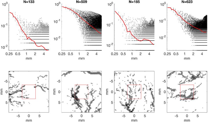
Our general approach is shown in Figure 3.The autocorrelation function B ( Δr ) is also found from the inverse Fourier transform of Equation
(12) to be B ( Δr ) = C ⋅ f ( b ) r
γ
and where γ = b − 3 for the convergence of the inverse transform
integral, 5 > b > 3 , and where C is a constant. Note that the integral operators (transform, average over
angles, and average over radii) are all linear so the order of these operations can be transposed for
computational
Acoustics 2019, 1 ease. 374
Our general approach is shown in Figure 3.
Figure 3. Derivation of isotropic scattering from a cylindrical element.
Figure 3. Derivation of isotropic scattering from a cylindrical element.
3. Methods
3. Methods
The fetal side placental perfusion was adapted from dual lobular placental perfusion methods
The fetal
previously side placental
published [19–21].perfusion was adapted
Briefly, human from
placentae dualnormal
from lobularterm
placental perfusion
deliveries were methods
obtained
previously
within published
5–10 min [19–21].
of delivery and Briefly,
examined human placentae
for tears and grossfrom normal
lesions. term25deliveries
Within were obtained
min, the umbilical artery
within
and vein5–10
weremin of delivery
cannulated and
near theexamined
insertion for tears
of the andongross
cord lesions.ofWithin
the surface 25 min,plate
the chorionic the umbilical
with five
artery and
French vein were
umbilical cannulated
catheters near the
for perfusion insertion
at 10–15 of the
mL min cordaon
−1 with the surface
finger of therate
pump. Flow chorionic plate
was adjusted
with five French umbilical catheters for perfusion at 10–15 mL min −1 with a finger pump. Flow
to maintain fetal vessel pressure at ~60 mmHg. The fetal perfusate consisted of M199 media without
rate was adjusted to maintain fetal vessel pressure at ~60 mmHg. The fetal perfusate consisted of
M199 media without phenol red (Gibco) modified by the addition of dextran (35–45 kDa; 30 mg/mL
fetal), D-Glucose (2 mg/mL), sulfamethoxazole (80 µg/mL), trimethoprim (16 µg/mL) gentamicin
(52 µg/mL), and heparin (20 USP IU/mL). The fetal perfusate was gassed with 20% O2 /75% N2 /5%
CO2 in a 250 mL vessel and bubbles trapped before delivery to the placenta. The cannulated placenta
was placed in a plastic bag and immersed in a 37 ◦ C water bath for an hour followed by Doppler and
ultrasound elastography experiments as described in McAleavey, et al. [22]. At the conclusion of these
experiments, the placenta was perfused with a 37 ◦ C suspension of 30% barium sulfate in 1% agarose
prepared from a 60% emulsion oral contrast suspension (Barium-Liquid E-Z-Pague; Bracco) diluted
with a 2% agarose in water solution with a gelling temperature of 35 ◦ C. Perfusion continued until
no further change was apparent. The placenta was then immersed in 10% neutral buffered formalin
for fixation before imaging with a Philips Brilliance 64 computerized axial tomography system. The
slice dimension was 768 × 768 pixels, each 0.25 × 0.25 mm; slice thickness: 0.67 mm, spacing between
slices: 0.33 mm.
4. Results
The raw data set (shown in the maximum intensity projections in the left panel of Figure 4) was
thresholded using a constant threshold limit of 180. The threshold was set at the minimum level
necessary to zero out the poorly vascularized edges of the placenta, while maintaining well connected
branches. Projections of the thresholded binary data can be viewed in the right panel of Figure 4. Also
shown in the right panel of Figure 4 is the convex hull of the placenta (solid black line) as well as the
boundary of the sampling region (dashed black line). The sampling region contains locations whereby
small autocorrelation sample cubes (6 mm on a side, or 27 × 27 × 21 voxels) can be translated along
any axis or diagonal by 6 mm without being outside the whole placenta’s boundary. For reference, thethresholded using a constant threshold limit of 180. The threshold was set at the minimum level necessary
to zero out the poorly vascularized edges of the placenta, while maintaining well connected branches.
Projections of the thresholded binary data can be viewed in the right panel of Figure 4. Also shown in
the right panel of Figure 4 is the convex hull of the placenta (solid black line) as well as the boundary of
the sampling region (dashed black line). The sampling region contains locations whereby small
Acoustics 2019, 1 sample cubes (6 mm on a side, or 27 × 27 × 21 voxels) can be translated along any axis375
autocorrelation or
diagonal by 6 mm without being outside the whole placenta’s boundary. For reference, the size of the
autocorrelation cubes is shown in the bottom right corner of the right panel of Figure 4, and the
size of the autocorrelation cubes is shown in the bottom right corner of the right panel of Figure 4, and
surrounding region that contributes to the autocorrelation spectrum is shown by the red circle of radius
the surrounding region that contributes to the autocorrelation spectrum is shown by the red circle of
9 mm.
radius 9 mm.
(a) (b)
Figure 4. (a) Maximum intensity projections of the raw data along the three primary axes. (b) Projections
Figure 4. (a) Maximum intensity projections of the raw data along the three primary axes. (b)
of the binary thresholded data along the three primary axes. Shown also is the convex hull (solid black
Projections of the binary thresholded data along the three primary axes. Shown also is the convex hull
line) and sampling region (dashed black line). The blue square in the bottom right shows the 6 mm × 6
(solid black line) and sampling region (dashed black line). The blue square in the bottom right shows
mm autocorrelation window and the red circle 9 mm in radius shows the region used to calculate the
the 6 mm × 6 mm autocorrelation window and the red circle 9 mm in radius shows the region used to
spectrum for each sample point.
calculate the spectrum for each sample point.
From within the sampling region, 1000 locations were chosen randomly as the center coordinate
of an autocorrelation window. Shifts were applied over all possible translations up to 6 mm, and
the autocorrelation function B(∆r ) = h I ( x, y, z) ∗ I ( x + ∆x, y + ∆y, z + ∆z)i was calculated, where
I ( x, y,pz) is the thresholded computed tomography (CT) intensity, as a binary function {1, 0}, and
∆r = ∆x2 + ∆y2 + ∆z2 . The normalized autocorrelation B(∆r )/B(0) was then calculated and used
in subsequent analyses.
Individual locations’ autocorrelation functions were found to be dependent on the number of
samples included within the 6 mm local cube, and this is related to the structure(s) included. For
example, a box centered on a large arterial segment has many pixels above threshold, and has a
rather slow decorrelation since the object I ( x ) is large. At the other extreme, if a box is centered on a
region with no obvious vascular architecture and only a few small isolated points above threshold,
the decorrelation is steep as a function of ∆r. These extremes point to the inherent difficulties in
characterizing a multi-scale process with limited sample volumes and limited resolution. For many
sample locations, however, a branching structure was included, and this corresponded to numbers of
voxels N above threshold between approximately N = 100 and 1000 (out of 15,309 voxels per cube).
These characteristic types are shown in Figure 5.
There is also a theoretical question relating to the nature of the autocorrelation function: Can it
reasonably be described as a power law function? To address this, power law functions were fit for
autocorrelation lags ∆r from 0 to 6 mm. The results of the power law coefficient for B(∆r ) = B0 · (∆r )γ
are plotted in Figure 6. The minimum mean squared error fit to a power law provides an exponent of
approximately −1.3. Some indication of a flattening at larger separation distances, greater than 4 mm,
was seen however larger multiscale analyses would be required to determine if that was a general
result indicating a tendency of the branching vasculature correlation function at longer ranges.decorrelation since the object I ( x ) is large. At the other extreme, if a box is centered on a region with
no obvious vascular architecture and only a few small isolated points above threshold, the decorrelation
is steep as a function of Δr . These extremes point to the inherent difficulties in characterizing a multi-
scale process with limited sample volumes and limited resolution. For many sample locations, however,
a branching structure was included, and this corresponded to numbers of voxels N above threshold
Acoustics 2019, 1 376
between approximately N = 100 and 1000 (out of 15,309 voxels per cube). These characteristic types are
shown in Figure 5.
Figure
Figure5.5.The
Thebottom
bottomrowrowshows
shows4 of the
4 of 1000
the regions
1000 regionsand thethe
and surrounding
surroundingneighborhood.
neighborhood. The The
top row
top
shows, for each
row shows, forregion, the normalized
each region, autocorrelation
the normalized for each
autocorrelation displacement
for (dots) as
each displacement well as the
(dots) wellaverage
as the
average
for
Acoustics for
FOReach
each 2radial
2019, binradial
PEER for a range
REVIEW ofa N
bin for = B (of0 )N (red
range = B(line).
0) (red line). 9
There is also a theoretical question relating to the nature of the autocorrelation function: Can it
reasonably be described as a power law function? To address this, power law functions were fit for
autocorrelation lags Δr from 0 to 6 mm. The results of the power law coefficient for B ( Δr ) = B0 ⋅ ( Δr )
γ
are plotted in Figure 6. The minimum mean squared error fit to a power law provides an exponent of
approximately −1.3. Some indication of a flattening at larger separation distances, greater than 4 mm, was
seen however larger multiscale analyses would be required to determine if that was a general result
indicating a tendency of the branching vasculature correlation function at longer ranges.
Figure
Figure6.6.Average
Averagenormalized
normalizedautocorrelation
autocorrelationfunction
functionfor
forregions
regionswith
with100
100Acoustics 2019, 1 377
Table 1. Average normalized autocorrelation power law fits as a function of upper and lower bounds
on occupied voxels, excluding extremely empty or filled samples.
Lower Bound N Upper Bound N Average Power Law γ
10 1000 −1.6
10 10,000 −1.5
100 1000 −1.3
100 10,000 −1.3
100 100,000 −1.3
5. Discussion
5.1. Consequence of the Model and Power Law
For soft tissue scattering, a number of studies have characterized the optical and acoustical
measurements of tissue specimens. Specifically, most carefully calibrated ultrasound backscatter
results from soft tissues report increasing backscatter with frequency. Generally this can be fit to a
power law with an exponent of 1 < γ < 2. For example, Campbell and Waag found liver backscatter
to increase as f 1.4 over the medical imaging band of 3–7 MHz [23] consistent with other pioneering
reports from the early 1980s [24–28]. Other examples of increasing backscatter vs. frequency in livers
are demonstrated in [29] extending up to 25 MHz, and in Lu et al. [30], also in livers. Similarly, for
other tissues, including sarcoma and carcinoma models, the increase in backscatter vs. frequency
was reported in Oelze and Zachary [31] and for thyroids in Rouyer et al. [32]. Thus, in assessing
our theoretical model, Equation (3), we are seeking a prediction of a backscatter power law fit of an
exponent slightly larger than one, given a relatively isotropic fractal fluid network scattering power
law of b − 2. In that case, it is clear that the power law b governing the number density of vessels
must be greater than 3. This is plausible, although reported data has to be considered in light of the
methodologies used; this was considered in Section 5.2. We also note for completeness that for F [q]2 /q
in spherical radial frequency being proportional to q(b−6) , also corresponds in the spatial domain to an
autocorrelation function proportional to 1/rsb−3 , where 3 < b < 5. For our placenta measurements,
γ = −1.3 = 3 − b implies b = 4.3, also implying backscatter would increase as k2.3 from Equation (13),
over some frequency range.
Although our resolution was limited by the CT system and contrast enhancement, optical studies
can obtain finer resolution. Schmitt and Kumar [33] studied phase contrast images of mouse liver
histology slides and found a power law power spectrum behavior for spatial frequencies down to at
least 1/10 microns.
Similarly, Rouyer et al. [32] studied thyroid tissue using broadband ultrasound systems and by
replotting their data we can estimate a power law behavior between 6 MHz and 15 MHz, corresponding
to wavelengths down to 100 microns.
5.2. Refinement of Theory vs. Experiments
A more exact comparison of theory to experiment will require greater precision on two fronts,
the backscatter vs. frequency power law, and the fractal branching power law of the fluid channels,
for specific organs. For example, with respect to liver, Campbell and Waag [23] reported a backscatter
proportional to the frequency to the 1.4 power over a range around 5 MHz for beef liver samples.
These measurements and the analytical treatment of all system effects were highly rigorous, yet
confirmation of these results over a larger bandwidth and in conjunction with imaging of the samples
(ensuring avoidance of any unwanted ligaments or trapped bubbles, for example) would help to refine
this estimate.
The fractal branching behavior assumed in Equation (10) is a continuous number density of
cylinders represented as proportional to N0 /ab ; this forms a major assumption of this framework,
yet is not known precisely. In reviewing the literature results, it must be kept in mind that there areAcoustics 2019, 1 378
major distinctions running through different analyses, principally 2D vs. 3D, and also the type of
measurement utilized. Fractal dimension is limited by topographical dimension, so 2D analysis of
slices or projections will have a lower dimension than corresponding 3D measurements. Full 3D
measurements at high resolution are rare and difficult due to the demands on resolution and sheer
size of the imaging data. Some high quality and high resolution 3D assessments of the branching
vasculature have been rigorously acquired for the brain [34] and the placenta [35], however to our
knowledge there have not been any published results from 3D fractal analyses of the liver vasculature
at high resolution.
Adding to the uncertainty about the important power law parameter b, which defines the number
density of cylindrical vessels as a function of their radius, over the ensemble and in linear dimensions,
is the wide variety of measurement styles that are typically reported. This is a major source of possible
misinterpretation. Our power law parameter b, which governs the number density of vessels as a
function of diameter, is not the same as the fractal dimension measured by sandbox or related box
counting techniques. Even in the cases of older literature reports where the number of vessels were
painstakingly counted (see Figure 1 of [18] indicating a power law of approximately −2.7 over some
older studies, Table 1 of [36] indicating a power law of approximately −1.3 in pulmonary veins, or Table
4 of [37] suggesting a power law of −2.5 in pulmonary arteries), there are important methodological
details that can swing the assessment. For example, many counting schemes derive the number of
vessel vs. branch generation number 1, 2, 3 . . . as ordinal numbers. The slope of this curve is not
the same as our number density vs. radius curve. Other schemes count “greater than or equal to”
a varying radius, which corresponds to an integration. Since the integration of 1/ab is proportional
to 1/a(b−1) , this scheme inherently shifts and reduces the power law parameter by one. Similarly,
a scheme of “binning” together vessels by proportional limits over a log scale will shift the power
law. For example, counting all the vessels within ±15% of 0.1 mm, then all those within 15% of 1
mm, then all those within 15% of 10 mm, will effectively integrate the distribution within these bins,
again converting the continuous distribution to a discrete set with 1/a(b−1) relative distribution. For
all these reasons, it is plausible that some literature assessments of branching vascular parameters,
using different methodologies, may not be the same as number densities defined in our manner by the
parameter b. Clearly, high resolution data sets in 3D are required to better define this important factor
in soft tissues such as liver, thyroid, prostate, and others. The particular 3D shapes and autocorrelation
functions from these different organs may differ from the results found in the placenta, since the 3D
placenta has a unique relationship with the maternal uterine blood flow, so organ-specific parameters
are needed to form baseline values.
6. Conclusions
High resolution contrast CT studies of a normal placenta’s branching vasculature in 3D
demonstrated a power law behavior for the 3D spatial autocorrelation function with an exponent close
to −1.3. Correspondingly, a theoretical hypothesis about scattering from tissue was generated from a
primitive cylindrical shape representing the plausible distribution of extracellular fluids and blood in
long fluid-filled channels throughout normal soft tissue. Assuming a wide range of diameters of the
cylindrical fluid spaces and a macroscopically isotropic distribution over some region of interest within
the organ, the predicted backscatter is of the form of a power law with dimension greater than one.
This matches some observations about the nature of vessels and measurements of backscatter from
soft tissues and is consistent with the power law autocorrelation function measured experimentally
from the placenta.
Pathologies that affect tissue morphology would be expected to modify this model in significant
ways, but it is prudent to first establish an accurate working model of normal soft tissue scattering.
More precise measurements of the key parameters will be required to fully test this hypothesis and
prior models based on spheres.Acoustics 2019, 1 379
Author Contributions: Theory and conceptualization, K.J.P.; imaging methodology, R.W.W.; software and formal
analysis, J.J.C.-N.
Funding: This research was supported by the Hajim School of Engineering and Applied Sciences at the University
of Rochester, by the National Institutes of Health grant number R21EB025290, and by the continued support of
placental investigations by the Mae Stone Goode Foundation.
Acknowledgments: The authors are deeply appreciative of perspectives on key theoretical issues from N. Baddour
and J. Astheimer. The authors thank R.K. Miller and C. Stodgell for performing these perfusions.
Conflicts of Interest: The authors declare no conflict of interest.
Appendix. Particular Form of Fourier Transform Pairs
Consistent with Bracewell [16], we use the following convention:
(a) Fourier transform in one dimension:
R∞
F (s) = f ( x )e−i2πxs dx = ={ f ( x )}
−∞
R∞ (A1)
f (x) = F (s)e+i2πxs ds
−∞
(b) Fourier transform/Hankel transform for cylindrical symmetry:
R∞
F (ρ) = 2π f (r ) J0 (2πρr )rdr = H{ f (r )}
0 (A2)
R∞
f (r ) = 2π F (ρ) J0 (2πρr )ρdρ
0
(c) Three-dimensional Fourier transform with spherical symmetry:
2π
R∞ 3DS ={ f (r )}
F (q) = q f (r ) sin(2qr )rdr =
0 (A3)
2π
R∞
f (r ) = r F (q) sin(2qr )qdq
0
Within this convention, the transform variable has units of cycles/distance. Furthermore, the
3D spherical transform is identical to the kernel for Born scattering, Equations (1)–(3). Finally, using
these definitions, we find that a 3D spherically symmetric power law function b(r ) = 1/r b has the
transform:
bπ (b−3)
B(q) = 2b−1 · π · Γ[2 − b] sin q for1 < b < 3, (A4)
2
where Γ is the
n gamma
o function. Thus, for example, if b = 3/2, an eigenfunction of the transform
3DS 1 c
occurs: = r3/2 = q3/2 .
References
1. Debye, P.; Bueche, A.M. Scattering by an inhomogeneous solid. J. Appl. Phys. 1949, 20, 518–525. [CrossRef]
2. Morse, P.M.; Ingard, K.U. Theoretical Acoustics; Princeton University Press: Princeton, NJ, USA, 1987; Chapter
8.
3. Mandelbrot, B.B. Fractals: Form, Chance, and Dimension; W.H. Freeman: San Francisco, CA, USA, 1997; p. 365.
4. Bassingthwaighte, J.B.; Bever, R.P. Fractal correlation in heterogeneous systems. Phys. D 1991, 53, 71–84.
[CrossRef]
5. Glenny, R.W.; Robertson, H.T.; Yamashiro, S.; Bassingthwaighte, J.B. Applications of fractal analysis to
physiology. J. Appl. Physiol. 1991, 70, 2351–2367. [PubMed]Acoustics 2019, 1 380
6. Lin, M.Y.; Lindsay, H.M.; Weitz, D.A.; Ball, R.C.; Klein, R.; Meakin, P. Universality of fractal aggregates as
probed by light scattering. Proc. R. Soc. Lond. A 1989, 423, 71–87.
7. Javanaud, C. The application of a fractal model to the scattering of ultrasound in biological media. J. Acoust.
Soc. Am. 1989, 86, 493–496. [CrossRef]
8. Shapiro, S.A. Elastic waves scattering and radiation by fractal inhomogeneity of a medium. Geophys. J. Int.
1992, 110, 591–600. [CrossRef]
9. Sheppard, C.J.R.; Connolly, T.J. Imaging of random surfaces. J. Mod. Optic. 1995, 42, 861–881. [CrossRef]
10. Lambert, S.A.; Nasholm, S.P.; Nordsletten, D.; Michler, C.; Juge, L.; Serfaty, J.M.; Bilston, L.; Guzina, B.;
Holm, S.; Sinkus, R. Bridging three orders of magnitude: Multiple scattered waves sense fractal microscopic
structures via dispersion. Phys. Rev. Lett. 2015, 115, 094301. [CrossRef]
11. Posnansky, O.; Guo, J.; Hirsch, S.; Papazoglou, S.; Braun, J.; Sack, I. Fractal network dimension and
viscoelastic powerlaw behavior: I. A modeling approach based on a coarse-graining procedure combined
with shear oscillatory rheometry. Phys. Med. Biol. 2012, 57, 4023–4040. [CrossRef] [PubMed]
12. Insana, M.F.; Wagner, R.F.; Brown, D.G.; Hall, T.J. Describing small-scale structure in random media using
pulse-echo ultrasound. J. Acoust. Soc. Am. 1990, 87, 179–192. [CrossRef]
13. Ishimaru, A. Wave Propagation and Scattering in Random Media; Academic Press: New York, NY, USA, 1978;
Volume 2, p. 572.
14. Campbell, J.A.; Waag, R.C. Ultrasonic scattering properties of three random media with implications for
tissue characterization. J. Acoust. Soc. Am. 1984, 75, 1879–1886. [CrossRef]
15. Parker, K.J. Hermite scatterers in an ultraviolet sky. Phys. Lett. A 2017, 381, 3845–3848.
16. Bracewell, R.N. The Fourier transform and its applications. In The Fourier Transform and Its Applications;
McGraw-Hill: New York, NY, USA, 1965; Chapter 12.
17. Baddour, N. Operational and convolution properties of three-dimensional Fourier transforms in spherical
polar coordinates. J. Opt. Soc. Am. A Opt. Image Sci. Vis. 2010, 27, 2144–2155. [CrossRef]
18. Krenz, G.S.; Linehan, J.H.; Dawson, C.A. A fractal continuum model of the pulmonary arterial tree. J. Appl.
Physiol. 1992, 72, 2225–2237. [CrossRef]
19. Miller, R.K.; Wier, P.J.; Maulik, D.; di Sant’Agnese, P.A. Human placenta in vitro: Characterization during 12
h of dual perfusion. Contrib. Gynecol. Obstet. 1985, 13, 77–84.
20. Miller, R.K.; Mace, K.; Polliotti, B.; DeRita, R.; Hall, W.; Treacy, G. Marginal transfer of ReoPro (Abciximab)
compared with immunoglobulin G (F105), inulin and water in the perfused human placenta in vitro. Placenta
2003, 24, 727–738. [CrossRef]
21. Menjoge, A.R.; Rinderknecht, A.L.; Navath, R.S.; Faridnia, M.; Kim, C.J.; Romero, R.; Miller, R.K.;
Kannan, R.M. Transfer of PAMAM dendrimers across human placenta: Prospects of its use as drug carrier
during pregnancy. J. Control. Release 2011, 150, 326–338. [CrossRef]
22. McAleavey, S.A.; Parker, K.J.; Ormachea, J.; Wood, R.W.; Stodgell, C.J.; Katzman, P.J.; Pressman, E.K.;
Miller, R.K. Shear wave elastography in the living, perfused, post-delivery placenta. Ultrasound Med. Biol.
2016, 42, 1282–1288. [CrossRef]
23. Campbell, J.A.; Waag, R.C. Measurements of calf liver ultrasonic differential and total scattering cross
sections. J. Acoust. Soc. Am. 1984, 75, 603–611. [CrossRef]
24. Bamber, J.C.; Hill, C.R. Acoustic properties of normal and cancerous human liver—I. Dependence on
pathological condition. Ultrasound Med. Biol. 1981, 7, 121–133. [CrossRef]
25. Nicholas, D. Evaluation of backscattering coefficients for excised human tissues: Results, interpretation and
associated measurements. Ultrasound Med. Biol. 1982, 8, 17–28. [CrossRef]
26. Lizzi, F.L.; Greenebaum, M.; Feleppa, E.J.; Elbaum, M.; Coleman, D.J. Theoretical framework for spectrum
analysis in ultrasonic tissue characterization. J. Acoust. Soc. Am. 1983, 73, 1366–1373. [CrossRef]
27. D’Astous, F.T.; Foster, F.S. Frequency dependence of ultrasound attenuation and backscatter in breast tissue.
Ultrasound Med. Biol. 1986, 12, 795–808. [CrossRef]
28. Reid, J.M.; Shung, K.K. Quantitative measurements of scattering of ultrasound by heart and liver. In
Ultrasonic Tissue Characterization II; Special Publication 525; National Bureau of Standards, U.S. Government
Printing Office: Washington, DC, USA, 1979.
29. Ghoshal, G.; Lavarello, R.J.; Kemmerer, J.P.; Miller, R.J.; Oelze, M.L. Ex vivo study of quantitative ultrasound
parameters in fatty rabbit livers. Ultrasound Med. Biol. 2012, 38, 2238–2248. [CrossRef]Acoustics 2019, 1 381
30. Lu, Z.F.; Zagzebski, J.A.; Lee, F.T. Ultrasound backscatter and attenuation in human liver with diffuse disease.
Ultrasound Med. Biol. 1999, 25, 1047–1054. [CrossRef]
31. Oelze, M.L.; Zachary, J.F. Examination of cancer in mouse models using high-frequency quantitative
ultrasound. Ultrasound Med. Biol. 2006, 32, 1639–1648. [CrossRef] [PubMed]
32. Rouyer, J.; Cueva, T.; Yamamoto, T.; Portal, A.; Lavarello, R.J. In vivo estimation of attenuation and
backscatter coefficients from human thyroids. IEEE Trans. Ultrason. Ferroelectr. Freq. Control 2016, 63,
1253–1261. [CrossRef] [PubMed]
33. Schmitt, J.M.; Kumar, G. Turbulent nature of refractive-index variations in biological tissue. Opt. Lett. 1996,
21, 1310–1312. [CrossRef] [PubMed]
34. Risser, L.; Plouraboue, F.; Steyer, A.; Cloetens, P.; le Duc, G.; Fonta, C. From homogeneous to fractal normal
and tumorous microvascular networks in the brain. J. Cereb. Blood Flow Metab. 2007, 27, 293–303. [CrossRef]
[PubMed]
35. Parker, K.J.; Ormachea, J.; McAleavey, S.A.; Wood, R.W.; Carroll-Nellenback, J.J.; Miller, R.K. Shear wave
dispersion behaviors of soft, vascularized tissues from the microchannel flow model. Phys. Med. Biol. 2016,
61, 4890. [CrossRef]
36. Gan, R.Z.; Tian, Y.; Yen, R.T.; Kassab, G.S. Morphometry of the dog pulmonary venous tree. J. Appl. Physiol.
1993, 75, 432–440. [CrossRef]
37. Singhal, S.; Henderson, R.; Horsfield, K.; Harding, K.; Cumming, G. Morphometry of the human pulmonary
arterial tree. Circ. Res. 1973, 33, 190–197. [CrossRef]
© 2019 by the authors. Licensee MDPI, Basel, Switzerland. This article is an open access
article distributed under the terms and conditions of the Creative Commons Attribution
(CC BY) license (http://creativecommons.org/licenses/by/4.0/).You can also read