Quantum optics meets black hole thermodynamics via conformal quantum mechanics: II. Thermodynamics of acceleration radiation
←
→
Page content transcription
If your browser does not render page correctly, please read the page content below
Quantum optics meets black hole thermodynamics
                                                                        via conformal quantum mechanics:
                                                           II. Thermodynamics of acceleration radiation

                                           A. Azizi,1 H. E. Camblong,2 A. Chakraborty,3 C. R. Ordóñez,3, 4 and M. O. Scully1, 5, 6
                                                                    1
                                                                        Institute for Quantum Science and Engineering,
arXiv:2108.07572v1 [gr-qc] 17 Aug 2021

                                                            Texas A&M University, College Station, Texas, 77843, USA
                                                     2
                                                         Department of Physics and Astronomy, University of San Francisco,
                                                                         San Francisco, California 94117-1080, USA
                                             3
                                                 Department of Physics, University of Houston, Houston, Texas 77024-5005, USA
                                                             4
                                                                 Department of Physics and Astronomy, Rice University,
                                                                 MS 61, 6100 Main Street, Houston, Texas 77005, USA.
                                                                         5
                                                                             Baylor University, Waco, TX 76706, USA
                                                             6
                                                                 Princeton University, Princeton, New Jersey 08544, USA
                                                                                     (Dated: August 18, 2021)

                                                                                           Abstract
                                           The thermodynamics of “horizon brightened acceleration radiation” (HBAR), due to a random
                                         atomic cloud freely falling into a black hole in a Boulware-like vacuum, is shown to mimic the
                                         thermodynamics of the black hole itself. The thermodynamic framework is developed in its most
                                         general form via a quantum-optics master equation, including rotating (Kerr) black holes and for
                                         any set of initial conditions of the atomic cloud. The HBAR field exhibits thermal behavior at the
                                         Hawking temperature and an area-entropy-flux relation that resembles the Bekenstein-Hawking
                                         entropy. In addition, this general approach reveals: (i) the existence of an HBAR-black-hole
                                         thermodynamic correspondence that explains the HBAR area-entropy-flux relation; (ii) the origin
                                         of the field entropy from the near-horizon behavior, via conformal quantum mechanics (CQM).

                                                                                               1
I. INTRODUCTION
Two of the central pillars of black hole thermodynamics [1, 2] are the Bekenstein-Hawking
entropy SBH [3–5] and the Hawking radiation effect [6, 7], along with the Hawking temper-
ature TH . These results appear to be universal properties of any theory combining quantum
physics with gravitation. While their true origin is still elusive after almost five decades,
progress has been made with string theory [8] and loop quantum gravity [9]. Moreover, all
approaches suggest that the origin of the thermodynamics is related to the event horizon [2],
possibly in the form of a conformal field theory [10–13]. Furthermore, due to the equiva-
lence principle, related results have been identified in accelerated systems in the form of
the Fulling-Davies-Unruh effect and the associated Unruh temperature [14–16]. Additional
insights into these profound concepts are of great interest; thus, in this paper, we probe
deeper into some nontrivial connections between the thermodynamics of black holes and
acceleration radiation.
We use the foundational results of the first article in this series [17] to fully develop the
thermodynamics of “horizon brightened acceleration radiation” (HBAR) generated by a an
atomic cloud in free fall into a black hole in a Boulware-like vacuum, with random injec-
tion times. These results generalize to rotating black holes the quantum optics approach of
Ref. [18]. Most importantly, as in the preceding article [17], conformal quantum mechanics
(CQM) is shown to fully drive the thermodynamic behavior [19–23]. Such a symmetry-based
approach is appealing as it supports the notion that conformal invariance may play a cru-
cial role in a deeper understanding of black hole thermodynamics [10–13], and ultimately,
in a theory of quantum gravity. In essence, the ensuing thermodynamic framework relies
on the primary thermal properties that consist of the Hawking temperature and thermality
via a detailed-balance Boltzmann factor—these are common to both HBAR and black hole
thermodynamics. With these tools, this paper establishes the existence of formally identical
thermodynamic functional relationships, which we describe as the HBAR-black-hole ther-
modynamic correspondence and include the HBAR area-entropy-flux relation. In particular,
the HBAR entropy flux is proportional to the rate of change in horizon surface area due to
the photon emission, with the critical proportionality factor that is exactly 1/4.
The organization of this article is as follows. It involves two intertwining tracks, properly
addressed in the different sections: the physics of the background gravitational field and
2HBAR
entropy
??
BH entropy
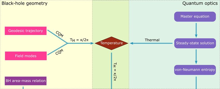
FIG. 1: Logical flow of basic concepts in this article. On the right hand side we have the elements of
quantum optics that leads to a thermal steady state. The black-hole (BH) geometry on the left side
assigns the temperature of the thermal steady state to be Hawking temperature via near-horizon
CQM. This assignment of temperature connects the BH aspects of the problem with the quantum
optics methodology. What remains to be explored is exactly how this relates to the BH entropy
on a deeper level.
the statistical quantum-optics approach leading to the thermodynamics through the master
equation for the reduced field density matrix. The logical progression of concepts and their
interrelationship are outlined in Fig. 1, with the details on the master equation briefly
summarized from the extensive treatment of Ref. [17]. In Section II, the basic concepts
for both tracks are introduced: the geometry, the interactions, and a review of the master
equation from Ref. [17]. In Sec. III, we show that the physics of the scalar field in the
gravitational background near the event horizon is governed by CQM; both the near-horizon
field equations and geodesics are derived. In Sec. IV, we examine the implications of the
governing physics of CQM, both in terms of the gravitational background and the master
3equation; in particular, this includes a derivation of the Planck form of the atom’s probability
of emission of photons, the existence of detailed balance Boltzmann factor associated with
the Hawking temperature, and a characterization of the thermal nature of the field state
via the master equation. These buildup of concepts culminates in Sec. V, with a thorough
analysis of the HBAR thermodynamics leading to the HBAR-black-hole thermodynamic
correspondence, and including the HBAR entropy flux formula of Ref. [18], with a general
proof of its conformal nature. Concluding remarks are given in Sec. VI, and followed by
the appendices, which include a summary of the Kerr geodesics (A) and the technicalities
of Kerr-geometry modes and vacuum states (B).
II. BASIC CONCEPTS: KERR GEOMETRY, ATOM-FIELD-GRAVITY INTER-
ACTIONS, AND FIELD MASTER EQUATION
A. Kerr geometry
The spacetime geometry provides the gravitational background where the atom-field in-
teractions take place. In this paper, we will focus on the geometry due to non-extremal
Kerr black holes, as these are of current interest and broad generality. as representatives
of the rotating class of black holes in 4D. Specifically, the Kerr metric describes the space-
time geometry that is the exact vacuum solution of the Einstein general relativistic field
equations in 4D in the presence of a black hole of mass M and angular momentum J. In
Boyer-Lindquist coordinates (t, r, θ, φ), the metric admits several equivalent expressions; in
its most basic form, in geometrized units c = G = 1, it is given by
(∆ − a2 sin2 θ) 2 4Mr ρ2 2 Σ2
ds2 = − dt − a sin2
θdtdφ + dr + ρ2
dθ 2
+ sin2 θdφ2 (1)
ρ2 ρ2 ∆ ρ2
where the Kerr parameter a = J/M, is the angular momentum per unit mass, and the
symbols ∆, ρ, and Σ are defined as
∆ = r 2 − 2Mr + a2 , ρ2 = r 2 + a2 cos2 θ ,
(2)
Σ2 = r 2 + a2 ρ2 + 2Mra2 sin2 θ = (r 2 + a2 )2 − ∆a2 sin2 θ .
The analysis of this paper is similarly valid for the Kerr-Newman geometry, which has the
same structural form form with an additional black hole electric charge Q, which shows up
4as a modification ∆ = r 2 − 2Mr + a2 + Q2 , leading to a replacement a2 → a2 + Q2 in Eq. (5)
and ensuing equations.
An alternative form of the Kerr metric,
∆ρ2 2 ρ2 2 Σ2
ds2 = − dt + dr + ρ2
dθ 2
+ sin2 θ (dφ − ̟dt)2 , (3)
Σ2 ∆ ρ2
can be derived by absorbing the off-diagonal term gtφ in a shift of the angular coordinate φ,
such that
gtφ
̟=− (4)
gφφ
is interpreted as a position-dependent angular velocity [24]. Equation (4) is particularly
useful to understand the physics as the event horizon is approached, as we will further
analyze in Sec. III.
The roots of the equation g rr = 0, which amounts to ∆ = 0, give the locations of the
outer and inner event horizon,
r± = M ± (M 2 − a2 )1/2 . (5)
In addition, the ergosphere is the region between the outer event horizon and the outer
static limit, which is defined by the largest root of gtt = 0. The non-extremal geometry
that we study in this paper corresponds to the physical condition M > a, which amounts
to ∆′+ ≡ ∆′ (r+ ) = r+ − r− 6= 0, and where the prime stands for the radial derivative.
The symmetries of the metric (1) lead to the Killing vectors
ξ(t) = ∂t , ξ(φ) = ∂φ (6)
associated with the stationary and axisymmetric nature of the metric (independence with
respect to t and φ respectively). In addition, the particular combination ξ = ξ(t) + ΩH ξ(φ)
defines a Killing vector with respect to which the horizon H is a null hypersurface; see the
interpretation in Sec. III, in and around Eq. (19). Three most relevant geometrical and
physical properties of the black hole are the horizon area A, the surface gravity κ, and the
angular velocity ΩH . The horizon area is
Z
√ 2
A= gθθ gφφ dθdφ = 4π(r+ + a2 ) . (7)
The surface gravity, geometrically defined from the Killing vector ξ by the horizon value of
κ = −(∇µ ξν )(∇µ ξ ν )/2 at r+ , takes the form
∆′+
κ= 2
. (8)
2(r+ + a2 )
5The angular velocity of frame dragging defines the angular velocity of the black hole as the
limit
a a
ΩH = lim ̟ = 2
= . (9)
r→r+ r+ + a2 2Mr+
B. Atom-field-gravity interactions
In addition to the gravitational background of the Kerr geometry, our model involves the
two interacting systems: the atomic cloud and the quantum field, as discussed in Refs. [17,
18, 22, 23]. The basic interaction leading to acceleration radiation is modeled by means of a
dipole coupling of a scalar field Φ with a freely falling atom. The atoms are randomly injected
and are freely fall into the Kerr black hole through a Boulware-like vacuum. For the Kerr
metric, the definition of a Boulware-like vacuum is technically challenging because of the
superradiant modes [25, 26]; this is discussed briefly in Ref. [23] and in Appendix B in greater
detail. One simple approach to overcome this difficulty is the introduction of a boundary to
exclude the regions of asymptotic infinity, as discussed in Sec. IV; the alternatives including
the asymptotic regions are considered in Appendix B. Any such states qualify as Boulware-
like and permit the generation of the HBAR radiation considered in this paper.
The quantization of the scalar field is expressed as
X
Φ(r, t) = [as φs (r, t) + h.c.] , (10)
s
where h.c. stands for the Hermitian conjugate; and r = (r, θ, φ) denotes the spatial Boyer-
Lindquist coordinates for the metric (1). The lowering operator as annihilates the Boulware-
type vacuum, with corresponding field modes φs . The labeling of the field modes with the
symbol s refers to the complete set of “quantum numbers” (including the mode frequency
ω); for the Kerr geometry in 3 spatial dimensions, this is s = {ω, l, m}, where {l, m}
are the spheroidal number and the “magnetic” quantum number associated with angular
momentum.
The interaction of the field Φ of Eq. (10) with a given two-level atom can be modeled as
a weak-dipole coupling of strength g,
VI (τ ) = g Φ(r(τ ), t(τ )) σ , (11)
in which σ = σ− e−iντ + σ+ eiντ is the operator that causes atomic state transitions, with σ−
being the corresponding atomic lowering operator. Given at atom in its ground state |bi,
6the coupling (11) allows for the emission of a scalar photon with the simultaneous transition
of the atom to its excited state |ai; this process has a first-order perturbation probability
R
amplitude −igIe,s , where Ie,s = dτ h1s , a| VI (τ ) |0, bi, and the field ground state |0i and
the state |1s i with one photon in mode s are involved. Similarly, the absorption probability
R
amplitude is −igIa,s , where Ia,s = dτ h0, a| VI (τ ) |1s , bi. Thus, the emission and absorption
probabilities are given by
P Z 2
e,s 2
=g dτ φ(±);s (r(τ ), t(τ )) eiντ (12)
Pa,s
where φ(ǫ);s , with ǫ = ±, are functions selected from φs and φ∗s according to the convention
φ(±);s = φ∗s , φs (in that order).
C. Field density matrix and master equation
Our goal is to study the the thermal properties of the HBAR radiation field. In order to
find the field configuration that is generated by the falling atomic cloud in the Kerr geometry,
an additional ingredient is useful beyond the the geometry details and interactions discussed
above: the density matrix. This is needed to fully characterize the nature of the emerging
field state and to compute the thermodynamic properties. The details are fully worked in
the first article of this series [17], generalizing Refs. [27] and [28]; a brief summary follows
next. The key step consists in evaluating the rate of change of the reduced density matrix
(ρP ) of the field, due to the random injection of atoms. The reduced field density matrix is
obtained via partial tracing (over the atomic degrees of freedom) from the density matrix
of the composite system: ρP = TrA ρPA . At the same time, this requires enforcing an
averaging procedure with respect to the atomic cloud (distribution of injection times) in
going from the density matrix of one atom to that of the whole cloud. The resulting coarse-
grained field density matrix satisfies the multimode master equation [17]
Xn
ρ̇diag ({ n }) = − Re, j (nj + 1) ρdiag ({ n }) − nj ρdiag ({ n }nj −1 )
j (13)
o
+Ra, j nj ρdiag ({ n }) − (nj + 1) ρdiag ({ n }nj +1 ) ,
which is valid under the assumption that only the diagonal elements are relevant; this is the
case for random injection times. In Eq. (13), the emission and absorption rate coefficients
7are Re,j = r Pe,j and Ra,j = r Ra,j , with r being the atom injection rate; and the index
j is shorthand for a given mode sj , with the single-mode quantum numbers s chosen in
an ordered sequence. In addition, the diagonal elements of the density matrix are denoted
by ρdiag ({ n }) ≡ ρn1 ,n2 ,...;n1 ,n2 ,... , where the notation { n } ≡ { n1 , n2 , . . . , nj , . . . } is used
for the occupation number representation, along with { n }nj +q ≡ { n1 , n2 , . . . , nj + q, . . . }
(with q an integer-number shift). In Sec. IV, we will use Eq. (13) to establish the thermal
nature of the HBAR radiation field.
III. NEAR-HORIZON PHYSICS AND CONFORMAL QUANTUM MECHANICS
IN KERR GEOMETRY: FIELD EQUATIONS AND GEODESICS
Two direct consequences of the gravitational field are need for the calculations of the
HBAR radiation field: the equations satisfied by the scalar field modes and the geodesic
equations.
A scalar field with mass µΦ in a generic metric gµν ∂ν satisfies the Klein-Gordon equation
1 √
− µ2Φ Φ ≡ √ ∂µ −g g µν ∂ν Φ − µ2Φ Φ = 0 .
(14)
−g
The general form of the metric leads to a differential equation for the mode functions that
is a particular case of the Teukolsky equation [26]. Instead of tackling its general form, we
will mainly consider its particular near-horizon behavior, which leads to a simplified gov-
erning equation of motion for the field that highlights the physical role played by conformal
symmetry. In this section, following Ref. [23], we briefly discuss the near-horizon form of
the field modes.
The field modes can be found by the following procedure. The Kerr metric (1) has the
symmetries of independence with respect to t and φ (stationary and axisymmetric); this
implies the existence of the Killing vectors ∂t and ∂φ of Eq. (6). As a result, it can be
analyzed with the separation of variables
φs (r, Ω, t) = Rs (r)Ss (θ)eimφ e−iωt , (15)
Replacing Eq. (15) in Eq. (14) for the metric (1), the polar-coordinate angular equation is
satisfied by spheroidal wave functions [26, 29]. We will use the regular solutions, the oblate
spheroidal wave functions of the first kind Ss (θ) [29], with eigenvalues given by the separation
8costant Λs ; the normalized combination Zs (Ω) = (2π)−1/2 Ss (θ)eimφ is a spheroidal harmonic.
Then, the radial function R(r) becomes
2
(r + a2 )2 ω 2 − 4Mramω + a2 m2
d dR 2 2 2 2
∆ + − Λs − a ω − µΦ r R = 0 . (16)
dr dr ∆
In addition, we introduce a new set of coordinates
t̃ = t , φ̃ = φ − ΩH t , (17)
which define a corotating frame with the black hole’s angular velocity ΩH . At the same
time, we perform a concomitant separation of variables
φω̃lm (r, t) = R(r)S(θ)eimφ̃ e−iω̃t̃ , ω̃ = ω − mΩH , (18)
which is viewed by a locally corotating observer as a frequency shift. Equation (18) highlights
the shifted frequency ω̃ to be used for the remainder of this paper; its relevance is due to its
association with the Killing vector
ξ ≡ ξ(t̃) = ξ(t) + ΩH ξ(φ) , (19)
which is timelike near the event horizon and null on the event horizon. Instead, the original
Killing vector ∂t is spacelike near the horizon and throughout the interior of a region known
as the ergosphere, whose external boundary—the outer static limit—is defined as the locus
where ∂t or gtt is null. The timelike behavior of ξ(t̃) allows us to define positive frequency
modes near the horizon with respect to this Killing vector, from the condition ξ(t̃) φs = −iω̃φs .
(H)
The near-horizon expansion, denoted by ∼ , involves the use of the hierarchy x ≡ r−r+ ≪
r+ . This can be enforced with the substitutions
(H) (H)
∆(r) ∼ ∆′+ x [1 + O(x)] , ∆′ (r) ∼ ∆′+ [1 + O(x)] , ∆′′ (r) = ∆′+ = 2 . (20)
In particular, we will apply this procedure to both the field equations and the geodesics.
For the Klein-Gordon equation (14), with the expression for the Kerr metric given by
Eq. (3), in the near-horizon region, one can directly write
Σ2 ∂ ρ2
∂ 1 ∂ ∂ 1 ∂
− 2 + + ∆ + 2 2 Φ (21)
ρ ∆ ∂ t̃2 Σ2 sin2 θ ∂ φ̃2 ρ2 ∂r ∂r ρ ∂θ
2 2 2
(H) (r + a ) ∂ 1 ∂ ∂ (H)
∼ − + ∆ Φ ∼ 0; (22)
ρ2 ∆ ∂ t̃2 ρ2 ∂r ∂r
9(H)
this is governed by the leading behavior ∆(r) ∼ ∆′+ x, which extracts the radial-time sector
of the metric. Equation (22) yields
" 2 #
1 d d ω̃ 1 (H)
x + 2
R(x) ∼ 0 . (23)
x dx dx 2κ x
It is easy to verify that this near-horizon equation can also be derived from Eq. (16) with
additional algebra.
Equation (23) is conformally invariant and can be reduced to the standard form of CQM
with the Liouville transformation R(x) ∝ x−1/2 u(x); thus, the near-horizon reduced radial
function u(x) satisfies the differential equation
d2 u(x) λ
2
+ 2 [1 + O(x)] u(x) = 0 , (24)
dx x
where
1 ω̃
λ= + Θ2 , Θ= . (25)
4 2κ
As in Ref. [17], the Hamiltonian H = p2x /2 + Veff (x), where Veff (x) = −λ/x2 is classically
scale invariant and defines conformal quantum mechanics (CQM) with an enlarged SO(2,1)
symmetry group that includes H , the dilation operator D and the special conformal oper-
ator K.
Equation (24) leads to a basic set of solutions given by u(x) = x1/2±iΘ . These are out-
going/ingoing wave functions that possess a logarithmic-phase singular behavior associated
with scale invariance. When their time dependence is restored, these solutions give the
outgoing and ingoing CQM modes,
(H)
φs (r, Ω, t) ∼ Φ±
s
(CQM)
∝ x±iΘ Ss (θ)eimφ̃ e−iω̃t , (26)
where φ̃ is the redefined corotating azimuthal coordinate for spinning black holes. We will
use these CQM modes in Sec. IV to find the emission and absorption rates of the free-falling
atoms.
We now turn to a brief summary of relevant results of the near-horizon geodesics in the
Kerr geometry. These are the spacetime trajectories of the atoms in free fall—they are in
locally inertial systems in the black-hole background, according to general relativity. The
trajectories are required for the evaluation of the photon emission and absorption probabil-
ities in Eq. (12), which we will consider in the near-horizon approximation. The geodesic
10equations are derived and analyzed in Appendix A. Inspection of Eq. (12) shows that the
functional dependences xµ (τ ) are needed. Basically, the relationship between r and τ can
be easily determined in the near-horizon limit, leading to explicit expressions of the other
coordinates in terms of x = r − r+ . In short, the leading near-horizon relationship τ = τ (x)
is
(H)
τ ∼ −kx + O(x2 ) + const; , (27)
where k = ρ̂2+ /c0 ; and the relationships t = t(x) and φ = φ(x) take the forms
(H) 1
t ∼ − ln x − Cx + O(x2 ) , (28)
2κ
(H)
φ̃ ∼ αx + O(x2 ) . (29)
where the constants C and α are given in Appendix A. The derivation of the emission and
absorption probabilities in the next section shows that neither these constants nor k are
explicitly needed for the final radiation results.
IV. HBAR IN KERR GEOMETRY: CONFORMAL NATURE AND THERMAL
CHARACTERIZATION
A. Emission and absorption probabilities: conformal nature
Emission and absorption rates of scalar photons by freely falling atoms in the Kerr geom-
etry can be derived from the basic Eq. (12) with the outgoing CQM modes from Eq. (26),
∗
with the assignments φ(+);s ∼ [Φ+(CQM) ] and φ(−);s ∼ Φ+(CQM) ; then,
P Z xf 2
e,s (H) 2 2
∼ g k dx x∓iΘ e∓imφ̃(x) e±iω̃t(x) eiντ (x) (30)
Pa,s 0
where k = ρ̂2+ /c0 and we have kept the φ̃ dependence for consistency of near-horizon calcu-
lations in the presence of frame dragging. In Eq. (30), the near-horizon region is bounded,
in principle, by an approximate upper limit xf . In particular, when τ , t, and φ̃ are replaced
in the integrand of Eq. (30) with Eqs. (27), (28), and (29), the emission rate takes the form
Z xf 2
2 2
Re,s = r g k dx x−iω̃/κ e−iqx , (31)
0
where q = C ω̃ + kν + αm, with C and α given by Eqs. (A18) and (A19), respectively.
11The emission rate of Eq. (31) displays an integral that has been analyzed in Refs. [17,
22, 23] The conclusions of that analysis are as follows. First, the behavior of the integral
is controlled by the competition of the two oscillatory factors x−iω̃/κ and e−iqx , Second, the
factor x−iω̃/κ , which arises from the properties of CQM, oscillates wildly with a logarithmic
phase as the horizon is approached, with scale invariance governed by ω̃/κ = 2Θ, and is thus
responsible for the leading value of the integral. Third, the upper limit xf can be effectively
replaced by infinity as the oscillations of e−iqx average out to essentially zero. Consequently,
the final expression for the emission rate becomes
∞ 2
2πr g 2ω̃ 1
Z
2 2
Re,s = r g k dx x−iω̃/κ e−iqx = 2 2π ω̃/κ
, (32)
0 κν e −1
in which the approximation ν ≫ ω̃ is applied. The functional dependence of the emission
rate in Eq. (32) corresponds to a Planck distribution; in particular, it is insensitive to the
initial conditions of the atoms in the cloud because it does not depend on the constants k,
C, and α.
Moreover, while the outgoing CQM waves in Eq. (26), Φ+
s
(CQM)
∝ xiΘ Ss (θ)eimφ̃ e−iω̃t , give
the Planck-distribution form of Eq. (32), the ingoing waves Φ+
s
(CQM)
do not contribute due
to the cancellation of the logarithmic phases. An important consequence of this property
is that acceleration radiation with a Planckian distribution from a freely falling atom will
exist for any generic Boulware-like state |Bi, as a result of the nonzero conformal integral in
Eq. (32). In effect, all that is needed is the extraction of the outgoing part of any definition
of the field modes. For the implementation of this procedure, one simple choice of boundary
conditions and vacuum is to analyze the acceleration radiation and its associated HBAR
entropy consists in enclosing the system with a boundary or mirror inside the speed-of-light
surface (which is within the ergosphere) [30], thus removing the problematic superradiant
modes [26] and defining a unique state |BM i, as considered in the references under [31].
Alternatively, as analyzed in Appendix B, the conventional bases that define the past and
future Boulware states |B ∓ i [32, 33] require the selection of purely outgoing components—
these are φup − out +
ωlm for |B i and φωlm for |B i. The precise definitions and characterizations of
these states are reviewed in Appendix B. For the states |B ∓ i, the superradiant modes [25]
(for −mΩH < ω̃ < 0) need to be handled separately. But, most importantly, the outgoing
components can be identified as in Eq. (B15) for |B ± i. In short, all of the possible definitions
of a Boulware-like state—including in particular |BM i and |B ± i—directly yield the Planck-
12distribution form of Eq. (32) through the extraction of the outgoing components, with any
remaining ingoing components not contributing to the radiation.
Finally, the absorption rate Ra,s can be computed in a manner similar to the derivation
leading to the emission rate Re,s of Eq. (32). As it turns out, Ra,s is more directly derived
from Re,s via the replacements ω̃ → −ω̃, and m → −m; this is, from first principles, due to
the functional forms of the rates in Eq. (30). Thus,
2πrg 2ω̃ 1
Ra,s = 2 −2π ω̃/κ
= e2πω̃/κ Re,s , (33)
κν 1−e
which has remarkable consequences for the question of possible thermal behavior, as will be
shown next.
B. Thermal behavior
We will now analyze in detail the properties of the HBAR radiation field and its possible
thermal nature. This involves two levels. First, we will reexamine the emission and ab-
sorption rates to evaluate a candidate Boltzmann factor and its relationship to the Hawking
temperature. Second, we will conduct a more thorough analysis through the reduced field
density matrix.
The Planck distribution displayed by the emission rate in Eq. (32) suggests thermal
behavior—or at least, it has a universal form compatible with thermality for all modes
of the radiation field. This property can be further tested with the ratio emission over
absorption, which, from Eq. (33), is equal to
Re,s
= e−2πω̃/κ . (34)
Ra,s
This ratio has the form of a thermal state with detailed-balance Boltzmann factor
Re,s
= e−β ω̃ (35)
Ra,s
(in natural units where the Boltzmann constant is kB = 1), with temperature
κ
T = β −1 = −1
≡ βH = TH . (36)
2π
The value of the effective temperature defined by this procedure in Eq. (36) is the same
as the Hawking temperature of the black hole—and it agrees with the form of the Planck
distribution of Eq. (32).
13It should be noted that the “temperature” in the primary thermal properties of Eqs. (35)
and (36) does not appear to be merely an effective phenomenological parameter, but it is
good candidate for a thermodynamic temperature in detailed-balance relations. This is due
to the fact that it is a universal temperature defined for all modes in Eq. (35), which is
identical to the thermodynamic temperature of the black hole. In addition, the condition
displayed in Eq. (35) is a direct consequence of the equations of near-horizon CQM, and can
be traced to the same logarithmic form of the phase in all of its modes.
The thermal nature of the state of the HBAR radiation field, under the conditions defined
via CQM in Eqs. (35) and (36), can be fully characterized using the master equation for
the field density matrix. For a cloud of freely falling atoms, with random injection times,
the density matrix has a diagonal form and satisfies the master equation (13). This is the
procedure fully worked out in Ref. [17], and which we now summarize and generalize for the
Kerr geometry. In fact, the general properties of the density matrix in this approach are
essentially geometry-independent and apply equally well to the generalized Schwarzschild
and Kerr geometries.
In Eq. (13), the vanishing of the time derivative defines the steady-state density matrix
(SS)
ρdiag ({ n }). Finding the steady-state solution involves an effective procedure that consists
of the following steps. First, one starts by finding the single-mode steady state, which
satisfies
Re,s 1 −nj β ω̃j
ρ(SS)
n,n single−mode = 1− (Re,s /Ra,s )n = e , (37)
Ra,s Zj
−1
with Zj = 1 − e−β ω̃j . Second, the factorization
(SS)
Y
ρdiag ({ n }) = ρ(SS)
nj ,nj (38)
j
can be proposed because the multimode density matrix is expected to be composed of
independent single-mode pieces under the given injection-averaging condition. Third, the
fact that this is the correct state can be verified by direct substitution in Eq. (13). Fourth,
the effective temperature T = β −1 can be enforced from the Boltzmann factor. As a result,
(SS)
Y Re,j nj 1 Y −nj β ω̃j
ρdiag ({ n }) = N = e , (39)
j
Ra,j Z j
−1
where Z = N −1 = 1 − e−β ω̃j
Q Q
j Zj = j is the partition function. This is indeed
a thermal distribution at the Hawking temperature, according to Eqs. (35) and (36); in
(SS) −1
particular, it yields the steady-state average occupation numbers hnj i = eβ ω̃j − 1 .
14Two critical points should be highlighted: (i) the appearance of the shifted frequency ω̃
in all ensuing expressions describing the thermal behavior; (ii) the fact that the result is
critically dependent on the primary thermal properties of Eqs. (35) and (36): the Boltzmann
factor and the Hawking temperature, where both emerge from near-horizon CQM for all field
modes. The thermal state of Eq. (39) confirms and extends the validity of the steady-state
analysis and HBAR properties, including the entropy flux calculations, of Refs. [17, 18] for
Kerr black holes. Such surprising results show close parallels with the thermodynamics of
the black hole itself [18]. We now turn to an analysis of this all-important problem, with a
thorough treatment of HBAR thermodynamics.
V. HBAR THERMODYNAMICS: ENTROPY AND HBAR-BLACK-HOLE COR-
RESPONDENCE
A. From von Neumann to the thermodynamic entropy
In Sec. IV, we have derived the thermal steady-state density matrix directly from near-
horizon CQM, and generalized it to rotating black holes with arbitrary initial conditions
for the freely falling atoms. With these robust results, we can now proceed to find the
entropy rate of change or flux ṠP due to the generation of acceleration radiation or field
quanta (“photons”). This is the horizon brightened acceleration radiation (HBAR) entropy
proposed in Ref. [18], whose insightful procedure we will follow and generalize in this section.
In general, for any quantum system, starting from the von Neumann entropy, S =
−Tr [ρ ln ρ], its rate of change is simply given by Ṡ = −Tr [ρ̇ ln ρ]. For the radiation field,
the corresponding trace can be evaluated as
X X
ṠP = − ρ̇diag ({ n }) ln [ρdiag ({ n })] = − ρ̇n1 ,n2 ,...;n1 ,n2 ,... ln ρn1 ,n2 ,...;n1 ,n2 ,... , (40)
{n} n1 ,n2 ,...
in which we are considering the diagonal sum over all the states { n } associated with all
the field modes, as in Sec. IV. Near the steady-state configuration, the density matrix in the
(SS)
logarithm of Eq. (40) can be approximated to leading order with ρdiag from Eq. (39). Thus,
the entropy flux of Eq. (40) becomes
h i
(SS)
X XX
ṠP ≈ − ρ̇diag ({ n }) ln ρdiag ({ n }) = − ρ̇diag ({ n }) ln ρ(SS)
nj ,nj , (41)
{n} j {n}
15as follows from the factorization (38) and by reversing the order of the sums. As a reminder,
the resulting summation with respect to j is a shorthand for the sum over all the field-mode
numbers s = {ω̃, l, m}, i.e., the field frequencies ω̃ in addition to the angular quantum
numbers. It should be noted that it is essential to account for all the available frequencies
in appropriate sums that define the full-fledged thermodynamic behavior. The replacement
of the thermal steady-state density matrix, e.g., Eq. (37), in Eq. (41) implies that
XX
ρ̇diag ({ n }) nj β ω̃j − ln(1 − e−β ω̃j ) .
ṠP ≈ (42)
j {n}
Moreover, Eq. (42) can be interpreted by enforcing two conditions: the trace normalization
Tr [ρ] = 1 and the dynamic generalization of the occupation-number averages
X
hnj i ≡ nj ρdiag ({ n }) , (43)
{n}
where these quantities hnj i ≡ hns i are defined for each set of field-mode numbers s =
{ω̃, l, m}. It should be further stressed that Eq. (43) is a generalization of the steady-state
(SS) −1
average occupation numbers hnj i = eβ ω̃j − 1 ; as such, it is no longer given exactly by
the Planck distribution, in such a way that it can generate a nonzero flux through hn˙ s i =
6 0.
Moreover, the second-term in Eq. (42) vanishes, to the same order of approximation, due to
the constancy of trace normalization; and the first term yields the entropy flux
2π
hn˙ s i ω̃ = hn˙ s i ω̃ .
X X
ṠP ≈ βH (44)
κ
s={ω̃,l,m} s={ω̃,l,m}
where the unique Hawking temperature, Eq. (36), is explicitly used as a last step.
In Eq. (44), the product hn˙s i ω̃ is the portion of the energy flux carried away by the
photons of the acceleration radiation, at a given frequency, and measured in the corotating
frame. For a single photon, the corotating energy ω̃ = ω − ΩH m involves the energy ω
(measured by an asymptotic observer) and the axial component m of the angular momentum
(along the black hole’s rotational axis). Then, the total corotating energy flux is
Ẽ˙ P = hn˙ s i ω̃ = hn˙ s i ω − ΩH m = ĖP − ΩH J˙P,z ,
X X
(45)
s={ω̃,l,m} s={ω̃,l,m}
which involves a combination of the change in the total energy EP and axial angular mo-
mentum JP,z of the photons. Therefore, the HBAR von Neumann entropy flux becomes
ṠP = βH ĖP − ΩH J˙P,z ,
(46)
16or ṠP = βH Ẽ˙ P , which can be restated in the form of thermodynamic changes
(th)
δSP = βH δEP − ΩH δJP,z ≡ δSP , (47)
(th)
where SP is the thermodynamic entropy. In other words, under near-equilibrium con-
ditions, where the steady state is a good first-order approximation, the changes in the
HBAR von Neumann and thermodynamic entropies of the radiation field coincide, with
the functional changes of Eq. (47). More generally, going back to the von Neumann en-
tropy, S = −Tr [ρ ln ρ], we can repeat the steps above to calculate SP and directly verify
this result. In effect, replacing ρ̇diag ({ n }) by ρdiag ({ n }) in Eqs. (40)–(42), these steps
lead to the modified analogue of Eq. (44), which is SP = β(EP − FP ); here, FP is the
Helmholtz free energy, such that βFP = − ln Z = j ln 1 − e−β ω̃j , with a partition func-
P
tion Z defined in Eq. (39). The agreement with Eq. (44) is due to the fact that the changes
of this thermodynamic entropy with fixed temperature reduce to Eq. (47): the black hole
acts as a temperature reservoir where the Hawking temperature is fixed by its characteristic
parameters.
B. HBAR-black-hole thermodynamic correspondence
The entropy flux (46) reinforces the existence of universal thermodynamic relations that
are intrinsic to the black hole but have other manifestations through relevant probes. In
other words, there are other aspects of black hole thermodynamics that extend the standard
results and can be revealed by accessing the near-horizon physics. In particular, the vacuum
states are probes that can generate different forms of radiation. By selecting a Boulware-like
state, the existence of HBAR radiation and its associated entropy are revealed. Moreover,
the thermodynamic changes of the Bekenstein-Hawking black hole entropy,
δSBH = βH δM − ΩH δJ , (48)
in terms of the mass M and angular momentum J of the black hole, display a striking formal
similarity with the HBAR entropy flux of Eqs. (46) and (47): they are analog relations with
corresponding entropy, energy, and angular momentum variables; and they are subject to
−1
the Hawking temperature TH = βH of Eq. (36). Thus, there exists a thermodynamic
correspondence
β=βH
SP , EP , JP,z ←−−→ SBH , M, J . (49)
17In addition, these analog relations can be further extended to charged black holes (Kerr-
Newman geometry), with an additional charge variable. Incidentally, as in Eq. (47), the
quantity δ M̃ = δM − ΩH δJ is the black hole energy in the corotating frame. The correspon-
dence (49) is not coincidental because of two key properties: (i) both systems are described
by the first law of thermodynamics in terms of just energy (mass), angular momentum, and
any other relevant degrees of freedom consistent with no-hair theorems [26]; (ii) they share
the same unique Hawking temperature. In essence, in thermal equilibrium, the quantum
field macroscopically mimics the black hole degrees of freedom; and the black hole generates
a near-horizon background governed by CQM and encoding this characteristic temperature
[cf. arguments leading to Eq. (36)]. Therefore, both the HBAR and the black hole entropies
have a common origin via near-horizon conformal symmetry; and the field satisfies thermo-
dynamic relations formally identical to black hole thermodynamics. We will refer to this set
of properties as the HBAR-black-hole thermodynamic correspondence.
C. Area-entropy-flux relation and radiation correspondence
There is an additional intriguing consequence of the thermodynamic correspondence. As
−1
it was found by Hawking [6, 7], the assignment TH = βH = κ/2π of Eq. (36) fixes the
values of the relationship of the entropy to other thermodynamic variables in Eq. (48),
thus determining the correct proportionality constant in the Bekenstein-Hawking entropy
SBH = A/4, so that
1
δSBH = δA . (50)
4
2
This can be verified directly for a Kerr black hole, with area A = 4π(r+ + a2 ), which implies
the change δA = 8πδ M̃ /κ, where κ = ∆′+ /2(r+
2
+ a2 ); from the Hawking temperature (36),
its change δA is [26]
δA = 4βH (δM − ΩH δJ) . (51)
In other words, once the temperature is fixed, there is a unique entropy-area relation. Then,
the HBAR-black-hole thermodynamic correspondence and the Bekenstein-Hawking entropy-
area relation of Eq. (50) suggest the existence of an analog entropy-area relation for the
HBAR entropy,
1
ṠP = ȦP , (52)
4
18where ȦP is the magnitude of the change in the area of the event horizon due to the emission
of acceleration radiation. Further justification of the HBAR area-entropy-flux relation (52)
can be outlined as follows. From Eq. (51), the magnitude of the black hole area change is
˙ where δ M̃ = δM − Ω δJ. If this change |M̃|
|Ȧ| = 4βH |M̃|, ˙ is due to photon emission in
H
the amount |M̃|˙ = Ẽ˙ , then the black hole area changes by the following specific amount
P
due to acceleration radiation, and according to Eq. (47),
1
|ȦP | = 4βH Ẽ˙ P = 4ṠP =⇒ ṠP = ȦP , (53)
4
which is the anticipated result. The area-entropy-flux relation (52) is a surprising and con-
venient rule of thumb, with a geometric interpretation that restates the central result of
this paper: the thermodynamic HBAR entropy property of Eq. (47), which is mandated by
the von Neumann entropy of the radiation field and implies an HBAR-black-hole thermo-
dynamic correspondence. Most importantly, we have established the robust form of these
results under fairly general conditions (black hole geometry and initial conditions of the
falling atomic cloud). However, some aspects of the area-entropy-flux relation (52) need to
be qualified, as discussed below.
First, the HBAR radiation does not involve the photons and black hole alone, but it is
mediated by the interaction of the field with the atoms. When the atoms are accounted
for in the relevant equations of the radiation generation process, the energy and angular
momentum of the black hole are transferred to the radiation field, but subject to the following
conservation laws,
δM + δEP + δEA = 0 , (54a)
δJ + δJP,z + δJA,z = 0 , (54b)
where EA and JA,z are the energy and angular momentum of the atom, respectively. Equa-
tions (54a) and (54b) can be combined into an energy conservation statement in the coro-
tating frame,
(δM − ΩH δJ) + δ ẼP + δ ẼA = 0 , (55)
where δ ẼP and δ ẼA are the field and atom corotating energy changes, respectively. Then,
going back to Eq. (51), the black hole area change is Ȧ = 4βH M̃, ˙ and Eq. (55) leads to
Ȧ = −4βH Ẽ˙ P + Ẽ˙ A , which can be interpreted as giving two distinct contributions to the
black hole area changes
Ȧ = ȦP + ȦA , (56)
19with one area change associated with the radiation field as in Eq. (52), i.e.,
ȦP = −4βH Ẽ˙ P = −4SP , (57)
but also with an extra contribution associated with the atoms,
ȦA = −4βH Ẽ˙ A , (58)
Therefore, when stating the HBAR area-entropy-flux relation (52), the area change ȦP under
consideration is only a fraction of the total change in the black hole area.
Second, in Eqs. (56)–(58), one should be careful with the signs—this is the reason that
we need to use an absolute value in Eq. (52). In particular, there is indeed a sign reversal
for the radiation field: as it carries away positive corotating energy, this corresponds to a
decrease in the area of the black hole (and increase in the HBAR entropy), according to
Eq. (57). This paradoxical situation is similar to the well-known corresponding statement
for Hawking radiation. However, such statements do not contradict the generalized second
law of thermodynamics (GSL), which refers to the sum of the entropies and not to the
entropy of the black hole or of the radiation field alone; thus, δAP ∝ −SP < 0 is allowed.
It should be noted, however, that the atoms carry corotating energy and fall into the black
hole with δ ẼA < 0, thus yielding an area increase δAA > 0, according to Eq. (58). Typical
nonrelativistic atoms contribute, in magnitude, significantly more than the radiation, so
that the overall area of the black hole does increase—this net result is different from the
corresponding case for Hawking radiation.
Incidentally, if the atoms are injected sufficiently close to the event horizon, one could
consider an effective description in which they are merely mediators for the radiation process,
in such a way that, if they could be counted as part of the black hole for bookkeeping
purposes. This is consistent with the dominant role played by near-horizon CQM and the
fact that the horizon can be regarded as a thick membrane or stretched horizon [34, 35], and
as seen from the outside, the atoms appear to accumulate therein. In a very real sense, the
black hole is their inevitable destiny. Then, one could interpret that there is a decrease in
the black-hole area from the radiation emission alone.
Third, in Eq. (55), the black hole and radiation corotating energies can be directly re-
lated to the corresponding entropies via Eqs. (47) and (48). As a result, the generalized
second law of thermodynamics, δStotal = δSBH + δSA + δSP ≥ 0, implies the inequality
20
δSA ≥ βH δEA − ΩH δJA,z , but no further predictions are possible without accounting for
additional information about the atoms.
   In short, our detailed analysis of the HBAR entropy highlights the thermodynamic en-
tropy property of Eq. (47), which similarly states the equivalence of the von Neumann and
thermodynamic entropies of the acceleration radiation. In addition, the entropy of the ra-
diated photon field can be written in terms of the change in the area of the event horizon
via the HBAR area-entropy-flux relation (52) as part of a larger set of relations within an
HBAR-black-hole thermodynamic correspondence. In particular, the area-entropy-flux for-
mula (52) is structurally identical to the Bekenstein-Hawking (BH) entropy, with the correct
prefactor 1/4. However, this entropy of the radiation field is due to the photon generation
by the freely falling atoms—as such, it is apparently different from the intrinsic BH entropy,
which is solely due to the existence of an event horizon as part of the geometry of a black
hole.
   Similarly, the HBAR field is not the same as Hawking radiation, even though they share
many formally identical qualities. The former requires the presence of an atomic cloud as a
mediator for the radiation process, while the latter is intrinsic to the black hole. As a result
of the mediation process and the conservation laws (54a)–(55), the HBAR radiation field is
maintained only inasmuch as atoms are falling into the black hole, and is limited by the size
of the cloud—but, of course, one can imagine a steady-state random injection that keeps
the process going on indefinitely. As time goes by, for the HBAR process, the black hole
mass increases due to the dominant contribution of the falling atoms, while for the Hawking
effect, the black hole mass decreases in the well-known evaporation scenario. Despite these
differences associated with the concomitant HBAR mediation by the atoms, for the random-
injection conditions considered in this paper, both forms of radiation, as seen far from the
black hole, have identical properties. Specifically, they are both thermal and characterized
by the same (Hawking) thermodynamic temperature TH = κ/2π. Therefore, just as for the
other thermodynamic attributes, there is an HBAR-black-hole correspondence that extends
beyond Eq. (49) to also include the mapping

                                        β=βH
                        (HBAR field) ←−
                                      −→ (Hawking radiation)          .                    (59)

   The area law (52) and the correspondence defined by Eqs. (49) and (59) are suggestive
of even deeper connections between the HBAR entropy and radiation field on the one hand,

                                               21
and the BH entropy and Hawking radiation on the other hand. This is an intriguing prospect
that will be explored elsewhere.
VI. CONCLUSIONS
In this article, we have shown that the von Neumann HBAR entropy flux (time rate of
change of the entropy) due to the acceleration radiation of a cloud of randomly injected
atoms falling into a black hole, in a Boulware-like vacuum, takes a functional form that is
in agreement with a specific form of thermodynamic entropy. This peculiar HBAR entropy
is defined with degrees of freedom mimicking those of the black hole itself, and with a
temperature equal to the Hawking temperature. As a consequence, it generates a powerful
HBAR-black-hole thermodynamic correspondence, which also includes the suggestive area-
entropy-flux relation ṠP ∝ ȦP . This intriguing result has a striking formal similarity with
the intrinsic Bekenstein-Hawking entropy of the black hole, including the proportionality
constant 1/4. The origin of the HBAR entropy has been elucidated with the thermal steady-
state field density matrix of the acceleration radiation by the randomly injected atoms into
the Boulware-like vacuum state. Moreover, the thermal property of the field density matrix
is completely governed by the conformal near-horizon physics of the black hole. This is due
to the fact that the field modes near the horizon are described by the CQM Hamiltonian;
the scale symmetry of these modes is responsible for the thermality of the HBAR field,
which involves both the Hawking temperature and the HBAR-black-hole thermodynamic
correspondence, including the correct prefactor in the entropy formula.
The near-horizon treatment is also useful as a practical analytical tool since it provides
an asymptotically exact approximation (in the usual asymptotic WKB sense), which yields
a closed-form solution for the emission and absorption probabilities that define the effective
temperature. While we have illustrated its use for the specifics of acceleration radiation and
HBAR entropy, its scope and computational effectiveness are not limited to these applica-
tions.
In conclusion, this paper establishes both the nature of the acceleration radiation and
the HBAR-black-hole thermodynamic correspondence for a fairly large class of black hole
solutions and arbitrary initial conditions of the atomic cloud. Furthermore, in this work,
we have elucidated the connection between the near-horizon CQM modes and the conven-
22tional Boulware modes for both the generalized Schwarzschild and Kerr geometries. These
generalizations cover all black solutions in 4D and a variety of solutions in higher dimen-
sionalities, thus displaying the robustness of the framework. Possible future extensions of
this work include understanding the connection of the HBAR entropy with the BH entropy
and exploring the group-theoretical aspects of this problem.
Acknowledgments
M.O.S. and A.A. acknowledge support by the National Science Foundation (Grant No.
PHY-2013771), the Air Force Office of Scientific Research (Award No. FA9550-20-1-0366
DEF), the Office of Naval Research (Award No. N00014-20-1-2184), the Robert A. Welch
Foundation (Grant No. A-1261) and the King Abdulaziz City for Science and Technology
(KACST). H.E.C. acknowledges support by the University of San Francisco Faculty De-
velopment Fund. This material is based upon work supported by the Air Force Office of
Scientific Research under award FA9550-21-1-0017 (C.R.O. and A.C.).
Appendix A: Kerr geodesics
The geodesic equations can be reduced to their first-order form, written in terms of the
conserved quantities: the energy E = −pt = −ξ(t) · p, the angular momentum along z-
direction Lz = pφ = ξ(φ) · p (as follows from the 4-momentum p and the Killing vectors),
the invariant mass µ, and the Carter constant Q. The geodesic equations are then given by
dr p
ρ2 = − R(r) (A1)
dτ
dθ p
ρ2 = ± Θ(θ) (A2)
dτ
dφ ℓ a
ρ2 = − ae − P(r)
+ (A3)
dτ sin2 θ ∆
dt r 2 + a2
ρ2 = −a(ae sin2 θ − ℓ) + P(r) , (A4)
dτ ∆
with the auxiliary functions P(r), R(r), and Θ(θ) defined by
P(r) = e(r 2 + a2 ) − aℓ (A5)
R(r) = [P(r)]2 − ∆ r 2 + (ℓ − ae)2 + q
(A6)
23ℓ2
Θ(θ) = q − cos θ a2 (1 − e2 ) +
2
. (A7)
sin2 θ
Here, we have used specific (per unit mass) conserved quantities e = E/µ, ℓ = Lz /µ, and
q = Q/µ = (pθ /µ)2 + cos2 θ a2 (1 − e2 ) + (ℓ/sin θ)2 .
In our approach, we only need the near-horizon behavior of the trajectories, which we
extract with the hierarchical near-horizon expansion. In terms of the near-horizon variable
x = r − r+ . Using Taylor expansion around the horizon in terms of the variable x, the radial
geodesic equation (A1) becomes
dx (H)
q
ρ2+ ∼ − c20 − c1 x + O(x2 ) , (A8)
dτ
where ρ2+ ≡ ρ2+ (θ) = r+
2
+ a2 cos2 θ. The constants in Eq. (A8) are functions of the conserved
quantities of the motion and black hole parameters, and are given by
2
+ a2 (e − ΩH ℓ) = r+ 2
+ a2 ẽ
c0 = P(r+ ) = r+ (A9)
c1 = −4er+ c0 + ∆′+ r+
2
+ (ℓ − ae)2 + q ,
(A10)
where
ẽ = −ξ(t̃) · p = e − ΩH ℓ > 0 (A11)
is the energy in a frame rotating with the black hole’s angular velocity ΩH .
However, we cannot yet integrate Eq. (A8) to get the proper time in terms of x due to
its θ dependence through ρ2+ , where θ evolves with the proper time following Eq. (A2). This
issue can be resolved if there is a functional relationship between θ and x, independently
of the other variables; this is indeed the case, as combining Eqs. (A1) and (A2) yields the
separable differential equation
dr dθ
p .= ∓p (A12)
R(r) Θ(θ)
Moreover, the near-horizon expansion and a change of variables y ≡ cos θ reduce this equa-
tion to the form
dx (H)dy
p ∼ ∓p (A13)
c20
− c1 x Θ(y) (1 − y 2)
[where, by abuse of notation, we have used Θ(θ) ≡ Θ(y)]. Equation (A13) provides a solution
y(x) that can be written using elliptic integrals of the first kind; more general results can be
found in Ref. [36]. However, we can avoid using the full-fledged solution by extracting the
leading-order near-horizon term, which gives
(H)
y ∼ const + O(x) . (A14)
24(H)
Reverting to the θ coordinate, we get cos θ ∼ cos θ+ + O(x). Here θ+ is a constant value of
the polar coordinate, which can be interpreted as the value of θ at which the atom approaches
the event horizon. This subsequently leads to the replacement of ρ2+ → ρ̂2+ ≡ r+
2
+ a2 cos2 θ+ .
Any O(x) terms have been ignored because, after integration, they will yield additional
contributions of order O(x2 ). Therefore, after making the replacement ρ2+ → ρ̂2+ , Eq. (A8)
can be integrated to give the proper-time functional relationship τ = τ (x) to leading order,
(H)
τ ∼ −kx + O(x2 ) + const , (A15)
in which k = ρ̂2+ /c0 . Furthermore, the factors ρ2 (which are θ-dependent) in Eqs. (A3) and
(A4) can be removed through division by Eq. (A1); this gives the functional relationships
t = t(x) and φ = φ(x) by integration in the near-horizon limit,
(H) 1
t ∼ − ln x − Cx + O(x2 ) , (A16)
2κ
(H)
φ̃ ∼ αx + O(x2 ) . (A17)
Instead of finding φ, we have calculated φ̃ = φ − ΩH t (which can be obtained by combining
solutions for φ and t), because the CQM modes in Eq. (26) explicitly depend on this corotat-
ing azimuthal variable. Most importantly, even though both φ and t have logarithmic terms
proportional to ln x, these cancel out when combined into the locally well-defined coordinate
φ̃. Finally, the constants C and α can be computed by collecting all the O(x) terms arising
from the functions on the right-hand side of Eqs. (A1)–(A4); a straightforward calculation
gives
1 1 c1 2r+ (ẽ + ΩH ℓ) 1 ΩH 2
C= + 2 − − aes+ − ℓ (A18)
2κ 2 c20 R+ ẽ 2κR+2
ẽ
and
aes2+ − ℓ ΩH a − 1/s2+
r+
α = ΩH 2
− 2
, (A19)
κR+ R+ ẽ
2 2
where R+ = r+ + a2 and s+ = sin θ+ . The constants C, α, and k, as shown in Sec. IV, do
not play a direct role in the radiation formulas.
Appendix B: Boulware vacuum and field modes for the Kerr black hole
In this appendix, we address the issue of the nonuniqueness of a Boulware vacuum for the
Kerr metric. Specifically, for this metric, when the asymptotic-infinity regions are included
25in the spacetime manifold, the presence of superradiant modes precludes the existence of a
unique Boulware vacuum that is empty at both past (I − ) and future (I + ) null infinity—
see the details that follow in this appendix. It is noteworthy that, even though this is a
technical issue that needs to be addressed, as shown below and in Sec. IV, the use of a
generic Boulware-like vacuum in our setup is sufficient—the final results for the acceleration
radiation and the HBAR entropy are insensitive to whatever choice is made within this
apparent ambiguity.
We begin by discussing the conventional past (B − ) and a future (B + ) Boulware vacuum
states defined on the Cauchy surfaces I − ∪ H− and I + ∪ H+ respectively [26, 32, 33]. For
comparison purposes with the existing literature, instead of using the near-horizon variables
and CQM modes of our paper, one can describe the relevant physics with the equivalent
tortoise coordinate r∗ , defined by
dr∗ 1 ∆
= , where f ≡ 2 , (B1)
dr f (r) (r + a2 )
dr r 2 + a2 /∆. This coordinate choice is made so that the radial-
R
which implies that r∗ =
time sector of the metric appears as near-horizon conformally flat and pushes the horizon
radially to minus infinity. Notice that the scale factor f (r) plays the same role as the homol-
ogous factor in generalized Schwarzschild coordinates. In the corotating coordinates (18),
the radial function R(r) satisfies the wave equation
2
d 2
+ ω̃ R(r) = 0 . (B2)
dr∗2
Most importantly, Eq. (B2) with the tortoise coordinate is equivalent to its counterpart
with the regular Boyer-Lindquist radial variable (24). The ingoing and outgoing waves
n o
e−iω̃(t̃+r∗ ) , e−iω̃(t̃−r∗ ) in terms of r∗ correspond to the conformal ingoing/outgoing modes
x∓iΘ of CQM. More generally (for all regions of spacertime), the coordinate transformation
of Eq. (B1) converts the radial equation into the equivalent form
2
d
− V (r∗ ) R(r) = 0 , (B3)
dr∗2
with r∗ ∈ (−∞, ∞), the event horizon being located at r∗ = −∞, and the scattering problem
taking a conventional form with an asymptotic potential V (r∗ ) ≡ Vωlm (r∗ ) given by
−ω̃ 2
r∗ → −∞ (r → r+ )
V (r∗ ) ∼ . (B4)
−ω 2
r∗ → ∞ (r → ∞)
26You can also read