IPHC Management Strategy Evaluation for Pacific halibut (Hippoglossus stenolepis) - International Pacific Halibut Commission

IPHC-2021-AM097-11
 IPHC Management Strategy Evaluation for Pacific halibut (Hippoglossus stenolepis)
 PREPARED BY: IPHC SECRETARIAT (A. HICKS, P. CARPI, I. STEWART, & S. BERUKOFF; 18 DECEMBER 2020)

PURPOSE
To provide a description of the International Pacific Halibut Commission (IPHC) Management
Strategy Evaluation (MSE) framework and an evaluation of management procedures for
coastwide scale and distributing the TCEY to IPHC Regulatory Areas.

SUMMARY
The Management Strategy Evaluation (MSE) at the International Pacific Halibut Commission
(IPHC) has completed an evaluation of management procedures (MPs) relative to the coastwide
scale of the Pacific halibut stock and fishery and has developed a framework to investigate MPs
related to distributing the Total Constant Exploitation Yield (TCEY) to IPHC Regulatory Areas.
The MSE framework contains the Operating Model (OM) that simulates the Pacific halibut
population and fisheries, and the Management Procedure (MP) with a closed-loop feedback. A
four-region operating model was conditioned to match historical data and then simulated forward
in time with uncertainty and using eleven MPs, defined at the 15th Session of the IPHC
Management Strategy Evaluation Board (MSAB015), to determine distributed mortality limits.
There are many trade-offs between objectives and between IPHC Regulatory Areas that must
be considered in the evaluation. Biological sustainability objectives were met for all MPs, except
that the percentage of spawning biomass in IPHC Regulatory Area 4B was less than 2% in more
than 5% of the simulations for all MPs. This particular result may be due to a number of factors,
including a misspecification of the population dynamics in that Biological Region. Yield objectives
were similar for coastwide performance metrics but varied across IPHC Regulatory Areas
depending on the elements of the MPs. MPs were ranked higher with respect to stability
objectives when methods to dampen variability, such as constraints on the annual change in the
TCEY and averaging of stock distribution estimates, were included in the MP. Two MPs
performed the best. One (MP-D) allowed for increases in the fishing intensity to accommodate
agreements in 2A and 2B. The other (MP-J) used a moving five year average of stock distribution
estimates to distribute the TCEY. All MSE results and visualizations to evaluate the MPs are
available on the MSE Explorer online tool1.

1 INTRODUCTION
The Management Strategy Evaluation (MSE) at the International Pacific Halibut Commission
(IPHC) has completed an evaluation of management procedures (MPs) relative to the coastwide
scale of the Pacific halibut stock and fishery and has developed a framework to investigate MPs
that also include distributing the Total Constant Exploitation Yield (TCEY) to IPHC Regulatory
Areas. The TCEY is the mortality limit composed of mortality from all sources except under-26-

1The current MSE Explorer tool is updated at http://shiny.westus.cloudapp.azure.com/shiny/sample-apps/MSE-
Explorer/ and the results are archived at http://shiny.westus.cloudapp.azure.com/shiny/sample-apps/IPHC-MSE-
AM097/

 Page 1 of 49

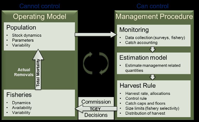
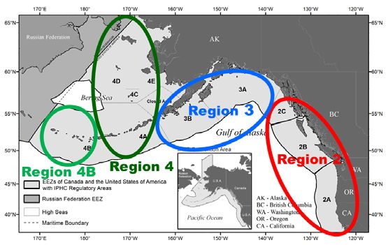
IPHC-2021-AM097-11

inch (66.0 cm, U26) non-directed commercial discard mortality, and is determined by the
Commission at each Annual Meeting for each IPHC Regulatory Area (Figure 1).
The development of this MSE framework aimed to support the scientific, forecast-driven study
of the trade-offs between fisheries management scenarios. Crafting this tool required:
 • the definition and specification of a multi-area operating model (OM);
 • an ability to condition operating model parameters using historical catch and IPHC
 Fishery-Independent Setline Survey (FISS) data and other observations;
 • identification and development of management procedures with closed-loop feedback
 into the operating model;
 • definition and calculation of performance metrics and statistics based on defined
 objectives to evaluate the efficacy of applied management procedures.
The MSE framework is briefly described below, followed by a description of the management
procedures being evaluated that distribute the TCEY to IPHC Regulatory Areas, and then the
presentation of simulation results.

2 FRAMEWORK ELEMENTS
The MSE framework includes elements that simulate the Pacific halibut population and fishery
(OM) and management procedures (MPs) with a closed-loop feedback (Figure 2). Specifications
of some elements are described below, with additional technical details in document IPHC-2020-
MSAB016-INF01.

2.1 Multi-area operating model
The generalized operating model is able to model multiple spatial components, which is
necessary because mortality limits and some objectives (Appendix I) are defined at the IPHC
Regulatory Area level (Figure 1). The OM is flexible, fast, modular, and easily adapted to many
different assumptions. It will be a useful tool for many investigations of the Pacific halibut fishery
in the future.

Figure 1: Biological Regions overlaid on IPHC Regulatory Areas. Region 2 comprises 2A, 2B,
and 2C, Region 3 comprises 3A and 3B, Region 4 comprises 4A and 4CDE, and Region 4B
comprises solely 4B.

 Page 2 of 49

IPHC-2021-AM097-11

Figure 2. Illustration of the closed-loop simulation framework with the operating model (OM) and
the management procedure (MP). This is the annual process on a yearly timescale.

2.1.1 Population and fishery spatial specification
The current understanding of Pacific halibut diversity across the geographic range of its stock
indicates that IPHC Regulatory Areas should be only considered as management units and do
not represent relevant sub-populations (Seitz et al. 2017). Therefore, four Biological Regions
(Figure 1) were defined with boundaries that matched some of the IPHC Regulatory Area
boundaries for the following reasons. First, data for stock assessment and other analyses are
most often reported at the IPHC Regulatory Area scale and are largely unavailable for sub-
Regulatory Area evaluation. Particularly for historical sources, there is little information to
partition data to a portion of a Regulatory Area. Second, it is necessary to distribute TCEY to
IPHC Regulatory Areas for quota management. If a Biological Region was not defined by
boundaries of IPHC Regulatory Areas (i.e. a single IPHC Regulatory Area is in multiple Regions)
it would be difficult to create a distribution procedure that accounts for biological stock distribution
and distribution of the TCEY to IPHC Regulatory Areas for management purposes. Further, the
structure of the current directed fisheries does not delineate fishing zones inside individual IPHC
Regulatory Areas, so there would be no way to introduce management at that spatial resolution.
To a certain degree, Pacific halibut within the same Biological Region share common biological
traits different from adjacent Biological Regions. These traits include sex ratios, age composition,
and size-at-age, and different historical trends in these data may be indicative of biological
diversity within the greater Pacific halibut population. Furthermore, tagging studies have
indicated that within a year, larger Pacific halibut tend to undertake feeding and spawning
migrations within a Biological Region, and movement between Biological Regions typically
occurs between years (Seitz et al. 2007; Webster et al. 2013).
Given the goals to divide the Pacific halibut stock into somewhat biologically distinct regions and
conserve the distribution of spawning biomass across the entire range of the Pacific halibut

 Page 3 of 49

IPHC-2021-AM097-11

stock, Biological Regions are considered by the IPHC Secretariat, and supported by the SRB
(paragraph 31 IPHC-2018-SRB012-R), to be the best option for biologically-based areas to meet
management needs. They also offer a parsimonious spatial separation for modeling inter-annual
population dynamics.
However, as mentioned earlier, mortality limits are set for IPHC Regulatory Areas and thus
directed fisheries operate at that spatial scale. Furthermore, since some fishery objectives have
been defined at the IPHC Regulatory Area level (Appendix I), the TCEY will need to be
distributed to that scale. Even though the population is modelled at the Biological Region scale,
fisheries can be modelled at the IPHC Regulatory Area scale by using an areas-as-fleets
approach within Biological Regions. This requires modelling each fleet with separate selectivity
and harvest rates that operate on the biomass occurring in the entire Biological Region in each
year. The distribution of the population within a Biological Region is currently approximated
assuming specified proportions of the population in each IPHC Regulatory Area within a
Biological Region that are based on historical observations. These proportions are constant over
ages and time, and allow for the calculation of statistics specific to IPHC Regulatory Areas.
Future improvements to the framework will allow for different options such as modelling
proportions based on population attributes and accounting for year-to-year variability.
2.1.1.1 Recruitment
Recruitment at age 0 to the population is determined at the coastwide level and is a function of
the coastwide spawning biomass using a Beverton-Holt spawner-recruit relationship with a
steepness of 0.75. The recruitment to each Biological Region is simply a proportion of the
coastwide recruitment and those proportions (constrained to sum to 1) are time-invariant.
Variability is incorporated as described below.
2.1.1.2 Fisheries
Fisheries were defined by IPHC Regulatory Areas (or combinations of areas if fishing mortality
in that area was small) and for five general sectors, which are consistent with the definitions in
the recent IPHC stock assessment (IPHC-2020-AM096-09 Rev_2):
 • directed commercial representing the O32 mortality from the directed commercial
 fisheries including O32 discard mortality;
 • directed commercial discard representing the U32 discard mortality from the directed
 commercial fisheries, comprised of Pacific halibut that die on lost or abandoned fishing
 gear, and Pacific halibut discarded for regulatory compliance reasons;
 • non-directed commercial discard representing the mortality from incidentally caught
 Pacific halibut in non-directed commercial fisheries;
 • recreational representing recreational landings (including landings from commercial
 leasing) and recreational discard mortality; and
 • subsistence representing non-commercial, customary, and traditional use of Pacific
 halibut for direct personal, family, or community consumption or sharing as food, or
 customary trade.

 Page 4 of 49

IPHC-2021-AM097-11

Thirty-three (33) fisheries were defined as a sector/area combination based on the amount of
mortality in the combination, data availability, and MSAB recommendations (Table 1).
The FISS is included as a fishery to output summaries of observations such as indices and
observed proportions-at-age in the population available to the FISS at a specific time and in a
specific region. Mortality from the FISS is included with the directed commercial fishery mortality,
although it could be kept separate. The fishery mimicking the FISS is simply referred to as
‘survey’ here to avoid confusion with actual FISS observations.
Selectivity determines the age composition of fishery mortality and ensures the removal of
appropriate numbers-at-age from the population when mortality occurs in the annual time-step.
Selectivity in this OM represents the proportion at each age that is captured and retained (i.e.,
landed) by the gear. Directed commercial discard mortality is modelled as a separate sector with
its own selectivity, and discard mortality for other sectors is included in the total mortality for
those sectors. Parameters for selectivity when conditioning models were determined from the
estimated parameters from the long Areas-As-Fleets (AAF) model in the recent stock
assessment (IPHC-2020-SA-01) including annual deviations in selectivity for the directed
fisheries and the survey. These parameters were modified to make the selectivity curves for
directed commercial fisheries and the survey asymptotic (i.e., no descending limb) because
movement should account for implied availability of a spatially explicit model compared to the
coastwide stock assessment. Selectivity could be further modified as necessary to improve fits
to data.
2.1.1.3 Weight-at-age
Empirical weight-at-age by region for the population, fisheries, and survey are determined using
observations from the FISS and the fisheries, as is done with the stock assessment models
(IPHC-2020-SA-02) and as described in detail in Stewart and Martell (2016). Smoothed
observations of weight-at-age from NMFS trawl surveys were used to augment weight-at-age
for ages 1–6 in the fishery sectors and survey. Population weight-at-age is smoothed across
years to reduce observation error. Finally, survey and population weight-at-age prior to 1997 is
scaled to fishery data because survey observations are limited if present at all.
2.1.1.4 Movement
Many data sources are available to inform Pacific halibut movement. Decades of tagging studies
and observations have shown that important migrations characterize both the juvenile and adult
stages and apply across all regulatory areas. The conceptual model of halibut ontogenetic and
seasonal migration, including main spawning and nursery grounds, as per the most current
knowledge, was presented in IPHC-2019-MSAB014-08 and was used to assist in parameterizing
movement rates in the OM.
In 2015, the many sources of information were assembled into a single framework representing
the IPHC’s best available information regarding movement-at-age among Biological Regions.
Key assumptions in constructing this hypothesis included:

 Page 5 of 49

IPHC-2021-AM097-11

 • ages 0-1 do not move (most of the young Pacific halibut reported in Hilborn et al. (1995)
 were aged 2-4),
 • movement generally increases from ages 2-4,
 • age-2 Pacific halibut cannot move from Region 4 to Region 2 in a single year, and
 • relative movement rates of Pacific halibut of age 2-4 to/from Region 4 are similar to those
 observed for 2-4-year-old Pacific halibut in Region 3, relative to older Pacific halibut.
Based on these assumptions, appreciable emigration is estimated to occur from Region 4,
decreasing with age. Pacific halibut age-2 to age-4 move from Region 3 to Region 2 and from
Region 4B to Regions 3 and 2, and some movement of older Pacific halibut is estimated to occur
from Region 2 back to Region 3 (Figure 3).
The conceptual model and assembled movement rates were used to inform the development of
the MSE operating model framework and were used as a starting point to incorporate variability
and alternative movement hypotheses in Pacific halibut movement dynamics. Movement in the
OM is modelled using a transition matrix as the proportion of individuals that move from one
Biological Region to another for each age class in each year.
2.1.1.5 Maturity
Spawning biomass for Pacific halibut is currently calculated from annual weight-at-age and a
maturity-at-age ogive that is assumed to be constant over years. There is currently no evidence
(IPHC-2020-SA-02) for skip spawning or maternal effects (increased reproductive output or
offspring survival for larger/older females) and therefore are not modelled but could be added.
Stewart & Hicks (2017) examined the sensitivity of the estimated biomass to a trend in declining
spawning potential (caused by a shift in maturity or increased skip spawning) and found that
under that condition there was a bias in both scale and trend of recent estimated spawning
biomass. The SRB document IPHC-2020-SRB016-07 tested maternal effects on estimates of
recruitment and concluded “there appears to be no evidence in the current data that the addition
of a simple age-based maternal effects relationship improves the ability of the current stock
assessment models to explain the time-series of estimated recruitments.” Ongoing research on
maturity and skip spawning will help to inform future implementations of the basis for and
variability in the determination of spawning output.

 Page 6 of 49

IPHC-2021-AM097-11

Table 1: The thirty-three fisheries in the OM, the IPHC Regulatory Areas they are composed of,
and the 2019 mortality (metric tonnes and millions of net pounds) for each.
 IPHC Regulatory 2019 Mortality 2019 Mortality
 Fishery Areas tonnes Mlbs
 Directed Commercial 2A 2A 404 0.89
 Directed Commercial 2B 2B 2,368 5.22
 Directed Commercial 2C 2C 1,665 3.67
 Directed Commercial 3A 3A 3,701 8.16
 Directed Commercial 3B 3B 1,048 2.31
 Directed Commercial 4A 4A 658 1.45
 Directed Commercial 4B* 4B 454 1.00
 Directed Commercial 4CDE 4CDE 748 1.65
 Directed Commercial Discards 2A 2A 14 0.03
 Directed Commercial Discards 2B 2B 59 0.13
 Directed Commercial Discards 2C 2C 27 0.06
 Directed Commercial Discards 3A 3A 145 0.32
 Directed Commercial Discards 3B 3B 68 0.15
 Directed Commercial Discards 4A 4A 41 0.09
 Directed Commercial Discards 4B 4B 14 0.03
 Directed Commercial Discards 4CDE 4CDE 32 0.07
 Non-directed Commercial Discards 2A 2A 59 0.13
 Non-directed Commercial Discards 2B 2B 109 0.24
 Non-directed Commercial Discards 2C 2C 41 0.09
 Non-directed Commercial Discards 3A 3A 748 1.65
 Non-directed Commercial Discards 3B 3B 218 0.48
 Non-directed Commercial Discards 4A 4A 159 0.35
 Non-directed Commercial Discards 4CDE 4CDE 1,588 3.50
 Non-directed Commercial Discards 4B 4B 68 0.15
 Recreational 2B 2B 390 0.86
 Recreational 2C 2C 857 1.89
 Recreational 3A 3A 1,674 3.69
 Subsistence 2B 2B 186 0.41
 Subsistence 2C 2C 168 0.37
 Subsistence 3A 3A 86 0.19
 Recreational/Subsistence 2A 2A 218 0.48
 Recreational/Subsistence 3B 3B 9 0.02
 Recreational/Subsistence 4 4A, 4CDE 27 0.06
 *The small amount of recreational and subsistence mortality from IPHC Regulatory Area 4B is included in
 Directed Commercial 4B

 Page 7 of 49

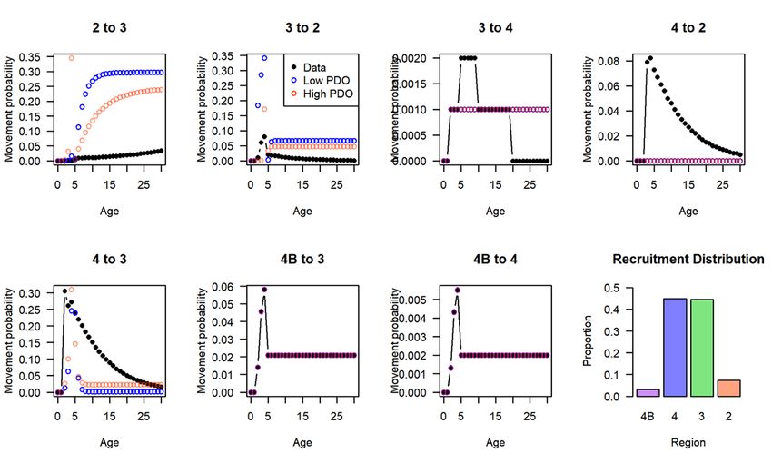
IPHC-2021-AM097-11

Figure 3: Estimated aggregate annual movement rates by age from Biological Regions (panels)
based on currently available data (from IPHC-2019-AM095-08).

2.1.2 Uncertainty and variability in the operating model
Uncertainty and variability are important to consider, as the goal of an MSE is to develop
management procedures that are robust to both. The OM should simulate potential states of the
population in the future, uncertainties within the management procedure, and variability when
implementing the management procedure.
2.1.2.1 Uncertainty in the conditioned OM
The conditioned OM is a representation of the Pacific halibut population and matches
observations from the fishery, FISS, and research. Uncertainty can be included in the OM by
varying parameters in two different ways. A common method method is to vary parameters
(Table 2) between simulated trajectories by randomly generating them from correlated
probability distributions that are derived from estimation procedures (e.g. the stock assessment).
A second method is to fix specific parameters at different values representing potential states.
Trajectories may be simulated using both methods and then integrated appropriately to produce
distributions of potential outcomes. At this time, the second method of fixing specific parameters
at alternative values is not being used but can easily be implemented in the future.
2.1.2.2 Projected population variability
Variability in the projected population is a result of initializing the population with a range of
parameters to recreate a range of historical trajectories and then including additional variability
in certain population processes in the projection. The major sources of variability in the
projections are shown in Table 3 and some are described in more detail below.

 Page 8 of 49

IPHC-2021-AM097-11

Table 2: Major sources of parameter uncertainty and variability in the conditioned operating
model (OM).
 Process Uncertainty
 Natural Mortality (M) Uncertainty determined from assessment
 Effect of the coastwide environmental regime shift based on the PDO and variability
 Average recruitment (R0)
 determined from conditioning
 Random lognormal deviations. Variability on distribution to Biological Regions
 Recruitment
 determined from conditioning
 Movement Uncertainty estimated when conditioning.

2.1.2.3 Linkage between average coastwide recruitment and environmental conditions
The average recruitment (R0) is related to the Pacific Decadal Oscillation index2, expressed as
a positive or negative regime (IPHC-2020-SA-02). The regime was simulated in the MSE by
generating a 0 or 1 to indicate the regime of each future year, as described in IPHC-2018-
MSAB011-08. To encourage regimes between 15 and 30 years in length (assuming a common
periodicity, although recent years have suggested less), the environmental index was simulated
as a semi-Markov process, where each subsequent year depends on recent years. However,
the probability of changing to the opposite regime was a function of the length of the current
regime, with a change probability equal to 0.5 at 30 years, and a probability near 1 at 40 or
greater years. This default parameterization results in simulated regime lengths most often
between 20 and 30 years, with occasional runs between 5 and 20 years or greater than 30 years.
This can be modified to test other scenarios.

Table 3. Major sources of projected variability in the operating model (OM).
 Process Variability
 Effect of the coastwide environmental regime shift, modelled as an autocorrelated
 Average recruitment (R0)
 indicator based on properties of the PDO
 Recruitment Random lognormal deviations.
 Annual and cohort deviations in weight-at-age by Biological Region, with approximate
 Size-at-age
 historical bounds
 Sector mortality allocation variability on non-directed commercial discard mortality,
 Sector mortality
 directed discard mortality, and unguided recreational mortality within an area
 Movement (variability) Change in parameters synchronized with simulated PDO-linked regime shift

2.1.2.4 Projected weight-at-age
Weight-at-age varies over time historically, and the projections capture that variation using a
random walk from the previous year. It is important to simulate time-varying weight-at-age
because it is an influential contributor to the yield and scale of the Pacific halibut stock. This
variability was implemented using the same ideas as in the coastwide MSE (IPHC-2018-
MSAB011-08), but was modified to incorporate autocorrelation in a more straightforward
manner, and allow for slight departures between regions and fisheries.

2 https://oceanview.pfeg.noaa.gov/erddap/tabledap/cciea_OC_PDO.htmlTable?time,PDO

 Page 9 of 49

IPHC-2021-AM097-11

The method used to simulate weight-at-age was described in IPHC-2020-SRB016-08 Rev1. Two
example projections are shown in Figure 4.

2.2 Conditioned four-region operating model
A multi-region OM was specified with four Biological Regions (2, 3, 4, and 4B; Figure 1), thirty-
three (33) fisheries (Table 1), and four (4) surveys. The model was initiated in 1888 and initially
parameterized using estimates from the long AAF assessment model.
Parameters for R0, the proportion of recruitment to each Biological Region, movement from 2 to
3, 3 to 2, and 4 to 3 were estimated by minimizing an objective function based on lognormal
likelihoods for spawning biomass predictions and region-specific modelled FISS indices,
robustified multivariate normal likelihoods for the proportion of FISS biomass in each region, and
observed proportions at age from the FISS. Other movement parameters were fixed to estimates
from data (Figure 3) except that movement probabilities from 4 to 2, 2 to 4, 4B to 2, and 2 to 4B
were set to zero for all ages. This makes the assumption that a Pacific halibut cannot travel
between these areas in an annual time step even though some movement from 4 to 2 at young
ages is predicted to occur from past data (Figure 3).

Figure 4: Past observed (shaded area) and two examples of possible one-hundred-year
projections of female weight at ages 5, 8, 12, 15, 20, and 25 in Biological Region 3.

The OM was conditioned using five sets of observations: the average estimated spawning
biomass from the long AAF and long coastwide stock assessment models (1888–1992),
estimated spawning biomass from the stock assessment ensemble including four models (1993–
2019), modelled FISS indices of abundance for each Biological Region, FISS proportions-at-age
for each Biological Region, and the proportion of “all selected sizes” modelled FISS biomass in
each Biological Region (all-sizes stock distribution).

 Page 10 of 49

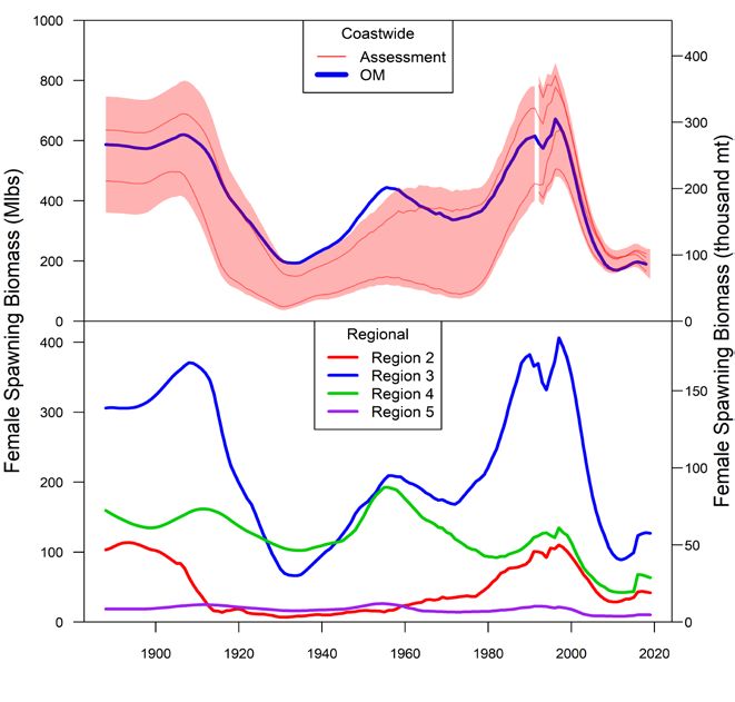
IPHC-2021-AM097-11

The predicted spawning biomass from the conditioned OM fell mostly within the range of
estimated spawning biomass from the four stock assessment models in the ensemble (Figure
5). The multi-region operating model predicted a female spawning biomass at the upper part
and slightly above the 90% credible interval from about 1930 to 1960 for the long assessment
models due to a large amount of predicted total biomass in Biological Regions 3 and 4. The
predicted stock distribution matched closely for most years, although the end of the time-series
in Biological Regions 2 and 3 and beginning of the time-series in Biological Regions 4 and 4B
showed departures. These departures from the observed stock distribution were consistent for
all models examined and suggest that the current structural specifications cannot capture these
trends, although preliminary estimates of stock distribution for 2020 are more consistent with the
OM (IPHC-2020-IM096-08).
Fits to the modelled FISS index were reasonable for all Biological Regions but showed some
patterns in residuals in Biological Region 2 (Figure 6). Few models that were examined were
able to fit the time-series in Biological Region 2 much better, and those that did show an
improved fit had poor fits to stock distribution.
Estimated and assumed movement probabilities-at-age from one Biological Region to another
are shown in Figure 7. Movement from 2 to 3 is estimated to be much greater than the data
suggest with higher movement of very young fish and lower movement rates of older fish during
high PDO regimes. The generally higher movement of older fish from 2 to 3 may be to counter-
balance the high movement rates of young fish from 3 to 2. The OM has movement rates near
5% for movement of older fish from 3 to 2. Younger fish tend to move at higher rates from 4 to
3 with little movement once they are age 8 and older. The OM assumes that this is a closed
population with no movement in or out of the four Biological Regions, which may explain some
of the differences observed from the movement rates based on observations.
The final OM shown here is a reasonable representation of the Pacific halibut population but has
some shortcomings. For example, the lack of fit to the 2019 stock distribution in Biological
Regions 2 and 3 (Figure 5) and the high predictions of young fish in Biological Region 2 in 2019
(Figure 6). The lack of fit to the proportions-at-age in 2019 are balanced by better fits in previous
years (not shown). There are many changes to the model and conditioning process that could
be made to potentially improve these fits. For example, movement may be sex-specific, but
tagging data are lacking this information.
Overall, the conditioned multi-region model represents the general trends of the Pacific halibut
population and is a useful model to simulate the population forward in time and test management
strategies.

 Page 11 of 49

IPHC-2021-AM097-11

Figure 5: Predicted coastwide spawning biomass (top left) where the blue line is the predicted spawning biomass from the
OM, the red lines are the predicted spawning biomass from each model in the stock assessment ensemble, and the red
shaded area is the 90% credible interval from the ensemble stock assessment. Total biomass by Biological Region in
millions of pounds (bottom left) where Region 4B is denoted by “Region 5”. Predicted annual proportions of biomass in each
Biological Region (right plots) from the conditioned OM (unfilled symbols) compared to the modelled FISS results (filled
circles) with 95% credible intervals.

 Page 12 of 49

IPHC-2021-AM097-11

Figure 6: Fits to modelled FISS NPUE index (four panels on the left) where filled circles are modelled FISS NPUE with 95%
credible intervals and the open triangles are predictions from the conditioned OM. Fits to proportions-at-age by sex and
Biological Region from the year 2019 (eight panels on the right) with filled circles connected by lines showing the proportions-
at-age determined from FISS data and the open circles showing predictions from the conditioned OM.

 Page 13 of 49

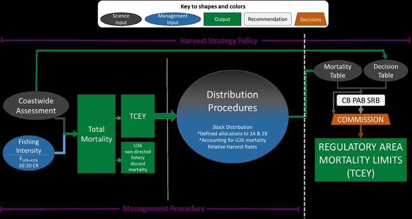
IPHC-2021-AM097-11

Figure 7: Probabilities of movement-at-age from the data and assumptions (as in Figure 3) and
the conditioned OM (blue and red circles for low and high PDO regimes, respectively). The
proportion of recruitment distributed to each Biological Region is shown in the lower right.

2.2.1 Uncertainty in the four-region operating model
Uncertainty in population trajectories was captured by adding variability to the parameters of the
operating model as specified in Table 2 with correlations between these parameters taken into
account. Different hypotheses of specific parameterizations (e.g. movement or steepness) may
be investigated through sensitivities and robustness tests.
Simulated trajectories of the OM with parameter variability show a wider range of female
spawning biomass than the 90% credible interval from the ensemble stock assessment (Figure
8). Prior to 1993, the trajectories are mostly within and above the upper portion of the ensemble
assessment 90% credible interval, but from 1993 to 2019 the trajectories encompass and extend
below and above the credible interval. Therefore, the OM is a reasonable representation of the
Pacific halibut population in recent decades and is modelled with variability that will allow for the
robust testing of MPs.

 Page 14 of 49

IPHC-2021-AM097-11

Figure 8: The 90% credible interval from six hundred trajectories of the OM with parameter
variability included (blue shaded area), shown against the 90% credible interval of the ensemble
stock assessment (two models before 1993 and four models for 1993–2019, red shaded area).
An example twenty trajectories are shown (thin blue lines) along with the median of all 600
trajectories (thick blue line).

The stock distribution with variability does not show a large departure from the observed stock
distribution (Figure 9). The variability is consistent with the observations except at the beginning
of the time-series in Biological Region 4 and in 2019 for Biological Regions 2 and 3. The
beginning of the time-series in Biological Region 4 was estimated with few data. The recent year
may have seen a shift in movement that is not explained by the OM, although preliminary
estimates of stock distribution for 2020 are more consistent with the OM (IPHC-2020-IM096-08).
Projections with the OM, incorporating parameter variability (Table 2) and projection variability
(Table 3), produced a wide range of trajectories. Figure 10 shows the median of six-hundred
simulations to 2119 without mortality due to fishing along with the interval between the 5th and
95th percentiles. Individual trajectories show that a single trajectory is highly variable and may
cover a wide range of that interval in this one-hundred-year projection period.

 Page 15 of 49

IPHC-2021-AM097-11

Figure 9: Stock distribution determined from FISS observations (points) and from the OM with
variability (shaded areas).

Figure 10: Six hundred 100-year simulations without fishing mortality. The dark blue line is the
median and the blue shaded area shows the interval between the 5th and 95th percentiles. The
thin blue lines denote the first 20 individual trajectories.

 Page 16 of 49

IPHC-2021-AM097-11

2.3 Management Procedures for coastwide scale and distribution of the TCEY
The management procedure consists of three elements (Figure 2): monitoring, estimation, and
the harvest rule. Monitoring (data generation) specifies the data collected from the stock that are
used by the estimation model (estimation) and the harvest rule to determine the total mortality,
the distribution of the TCEY to IPHC Regulatory Areas, and subsequent allocation to sectors.

2.3.1 Monitoring (data generation)
The MSE framework generates data by simulating the sampling process and can incorporate
variability, bias, and any other properties that are desired. Fishery data are generated as needed
by the estimation model (e.g., age compositions and CPUE). Data are generated from the survey
in the OM (NPUE, WPUE, age compositions, and stock distribution) that are used by the
estimation model and management procedures.

2.3.2 Estimation model
The Estimation Model (EM) is analogous to the stock assessment and introduces estimation
error in the simulations. Three approaches to introduce and investigate estimation error were
included in the MSE framework. Results from all three methods are available on the MSE
Explorer.
2.3.2.1 No estimation error
The estimates and predictions needed for the harvest rule are taken directly from the operating
model and do not include estimation error. This provides an indication of the best possible
outcome given the natural variability in the population, although it is unrealistic because
population quantities are never known without error, and therefore not presented here.
2.3.2.2 Simulate estimation error
This approach simulated the error in estimates and predictions needed for the harvest rule using
random number generation from probability distributions, as was done in the coastwide MSE.
The OM determines the stock status and the TM consistent with the input fishing intensity (i.e.
FSPR). Correlated deviates randomly generated with a bivariate normal distribution, including an
autocorrelation of 0.4 with previous deviates, were applied to the stock status and TM. Details
can be found in Section 4.2.2. of IPHC-2018-SRB012-08. This method is useful to provide a
reasonable approximation of the assessment process while speeding up the simulation process
and allowing investigation of specific levels of bias and variability.
2.3.2.3 Model estimation error
This method uses a model similar to the stock assessment (i.e. stock synthesis), but simplified,
with generated data to determine the estimates and predictions needed for the harvest rule. The
assessment models that this EM were based on are complex and developed for short-term
forecasts using currently available data. Increasing the number of years of data in the models,
possibly not simulated with the exact processes that the assessment was tuned to, can cause
the models to perform less than optimal. However, the use of an EM based on the assessment
models provides a more accurate representation of the assessment process and of the bias
associated with it. This method is currently in development and will be available for future
iterations of the MSE. Some results using only one of the four assessment models used in the

 Page 17 of 49

IPHC-2021-AM097-11

ensemble are available for preliminary comparison to the other methods, although are not
presented here.

2.3.3 Harvest Rule
The Harvest Rule contains additional procedures when determining the mortality limits, such as
the application of a control rule and distribution of the limits to IPHC Regulatory Areas. The
harvest rule for distributing the TCEY begins with the coastwide TCEY determined from the stock
assessment and fishing intensity defined by the reference SPR (with application of the control
rule). Figure 11 is an illustration of the current interim harvest strategy policy at IPHC, which
includes the harvest rule as part of the management procedure. The TCEY may be distributed
to Biological Regions first and then to IPHC Regulatory Areas, or directly to IPHC Regulatory
Areas. Relative adjustments can be applied in each step of the distribution process. Typically,
the distribution procedure does not appreciably alter the coastwide fishing intensity (although a
slight change may occur when applying distribution methods that differ greatly due to different
selectivity patterns accessing the population). However, there is interest in management
procedures that are only limited to being less than a maximum fishing intensity (i.e., above a
minimum SPR) that would account for modifications in the TM during the distribution procedures.

Figure 11: Illustration of the Commission interim IPHC harvest strategy policy (reflecting
paragraph ID002 in IPHC CIRCULAR 2020-007) showing the coastwide scale and TCEY
distribution components that comprise the management procedure. Items with an asterisk are
three-year interim agreements to 2022. The decision component is the Commission decision-
making procedure, which considers inputs from many sources.

 Page 18 of 49

IPHC-2021-AM097-11

The Coastwide TCEY is calculated from the TM by removing the U26 portion of the non-directed
discard mortality, which is approximated in the MSE framework by a fixed length-at-age key
determined from historical observations applied to non-directed discard mortality observed the
previous year.
The outputs of the management procedure are TCEY limits for each IPHC Regulatory Area,
which then need to be allocated to the different sectors specific to the IPHC Regulatory Area.
See Table 1 for a complete list of the fishing sectors by IPHC Regulatory Area. There are two
parts to the simulation procedure: the allocation of the upcoming mortality limits by sector, and
the calculation of the realized mortality by sector. The allocation of mortality limits is necessary
because some sector’s mortality limits are determined from the limits for other sectors. In the
current framework, the calculation of the realized mortality differs from the calculation of the
mortality limits for the non-directed discard, directed discard, subsistence, and unguided
recreational mortalities (i.e., implementation error). Mortality limits and realized mortality are
equal for the various recreational and directed commercial sectors (i.e. no implementation error
for these sectors).
The simulation procedure begins by subtracting the non-directed commercial O26 discard
mortality by IPHC Regulatory Area from the corresponding IPHC Regulatory Area TCEY, and
the remainder is then allocated to directed fishery sectors. Each IPHC Regulatory Area has a
unique catch-sharing plan (CSP) or allocation procedure, and these CSPs were mimicked as
closely as possible in the MSE framework. When the TCEY for an IPHC Regulatory Area is very
low, the CSP may no longer be applicable and alternative decisions may be necessary. It is
unknown what the allocation procedure may be at very low TCEYs (far below levels actually
observed in the historical time-series), so working with MSAB members, a simple assumption
was to assume that the sum of the directed non-FCEY components would not exceed the TCEY
without non-directed commercial O26 discard mortality, and the FCEY components would be
set to zero.
Overall, the estimated values from the data generation and estimation model/estimation error
steps are used in the application of the harvest rule to determine mortality limits by IPHC
Regulatory Area. The simulated application of the harvest rule will therefore include errors in
stock status as well as the size of the population, both of which are propagated into management
quantities.

2.3.4 Management procedures for evaluation
The MSAB has defined coastwide and distribution elements of management procedures that are
important for future evaluation, including the following listed in paragraph 42 of IPHC-2020-
MSAB015-R.

 Page 19 of 49

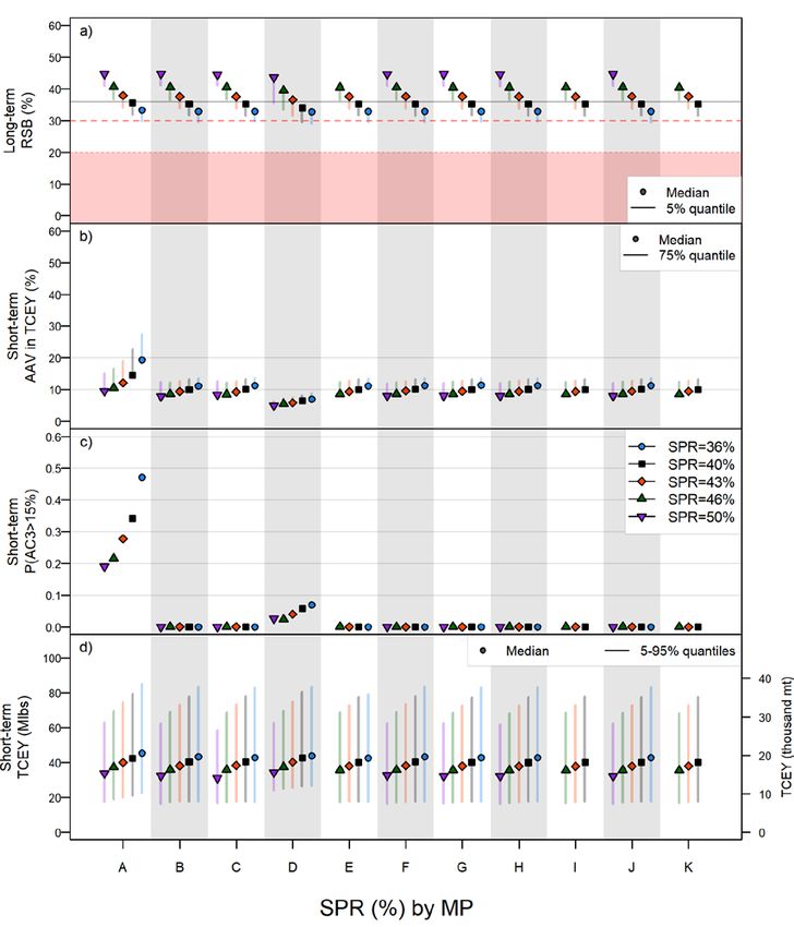
IPHC-2021-AM097-11

 IPHC-2020-MSAB015-R, para. 42.The MSAB AGREED that the following elements of
 interest for defining constraints on changes in the TCEY, and distribution procedures be
 considered for the Program of Work in 2020:
 a) constraints on the change in the TCEY can be applied annually or over multiple
 years at the coastwide or IPHC Regulatory Area level. Constraints on the change in
 TCEY currently considered include a maximum annual change in the TCEY of 15%,
 a slow-up fast down approach, multi-year mortality limits, and multi-year averages
 on abundance indices;
 b) indices of abundance in Biological Regions or IPHC Regulatory Area (e.g. O32 or
 All sizes from modelled survey results);
 c) a minimum TCEY for an IPHC Regulatory Area;
 d) defined shares by Biological Region, Management Zone, or IPHC Regulatory Area;
 e) maximum coastwide fishing intensity (e.g. SPR equal to 36% or 40%) not to be
 exceeded when distributing the TCEY;
 f) relative harvest rates between Biological Regions or IPHC Regulatory Areas.

At MSAB014 and MSAB015, elements specifying candidate management procedures were
defined for simulation and subsequent evaluation (Table 4 and Table II.1 in Appendix II,
reproduced from IPHC-2020-MSAB015-R).

3 CLOSED-LOOP SIMULATION RESULTS
For brevity, only the simulated estimation error results are reported to compare across SPR
values, and some figures and tables only present results using an SPR of 43%. Simulations with
alternative estimation error methods and additional SPR values are available on the interactive
MSE Explorer website. Pertinent results related to primary objectives are discussed below.
Figure 12 shows coastwide performance metrics linked to the primary coastwide objectives. The
relative spawning biomass (RSB) is similar across all management procedures, but varies with
SPR. All MPs are within the 10% tolerance for RSB dropping below 20% SPR (Table 5), and the
median RSB resulting from an SPR of 40% is slightly less than 36%. Table 5 shows that the
probability of being below 36% is slightly less for MP-A compared to all other MPs. The AAV
was higher for MP-A as well, especially at lower SPR values, because MP-A was the only MP
without an annual constraint of 15% on the TCEY. For the same reason, the probability that the
annual change (AC) was greater than 15% was greater than zero for MP-A and zero for all other
MPs, except MP-D which allowed the coastwide TCEY to accommodate agreements in 2A and
2B. Short-term median TCEY was between 30 and 50 Mlbs (13,600 and 22,700 t) for all MPs
and SPR values, with larger values for lower SPR values (higher fishing intensity) and slight
variations between MPs. The difference in the short-term median TCEY was less than 2.5 Mlbs
(1,100 t) between MPs for an SPR of 43% (Table 5).

 Page 20 of 49

IPHC-2021-AM097-11

Table 4: A comparison of management procedures (MPs) showing the elements included in defined MPs. See Appendix II
and Appendix III for additional details of the MPs.

 Element MP-A MP-B MP-C MP-D MP-E MP-F MP-G MP-H MP-I MP-J MP-K
 Maximum coastwide TCEY
 change of 15%

 Maximum Fishing Intensity
 buffer (SPR=36%)

 O32 stock distribution

 O32 stock distribution
 (5-year moving average)

 All sizes stock distribution

 Fixed shares updated in 5th
 year from O32 stock
 distribution
 Relative harvest rates of 1.0 for
 2-3A, and 0.75 for 3B-4

 Relative harvest rates of 1.0 for
 2-3, 4A, 4CDE, and 0.75 for 4B
 Relative harvest rates by
 Region: R2=1, R3=1, R4=0.75,
 R4B=0.75

 1.65 Mlbs fixed TCEY in 2A

 Formula percentage for 2B

 National Shares (2B=20%)

 Page 21 of 49

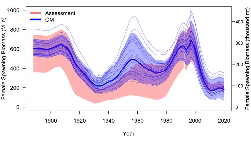
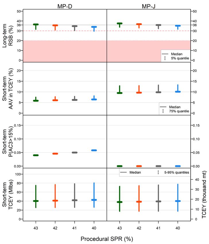
IPHC-2021-AM097-11

Short-term performance metrics for the TCEY in each IPHC Regulatory Area are shown in Figure
13 as well as Table 6, Table 7, and Table 8. These are the median-minimum and median-
average TCEY over a ten-year period and the median-minimum and median-average
percentage of TCEY in each IPHC Regulatory Area over a ten-year period (short-term). MPs F–
K show decreased TCEY in 2A and MPs E and G–K show decreased TCEY in 2B along with
increased TCEY in all other IPHC Regulatory Areas because the current agreements from 2A
and 2B, or national shares for 2B, are not included in those MPs. The TCEY increases in 3B,
4A, and 4B with the increased relative harvest rate included in MP-H and MP-K, while it
decreases in other IPHC Regulatory Areas. MP-J, which uses a 5-year average of stock
distribution, shows similar TCEY values as MP-G, but with lower AAV for most IPHC Regulatory
Areas (Table 8). Stability related performance metric differences are evident at the IPHC
Regulatory Area level with MP-J, even though its stability was not much different than that of
MP-G at the coastwide level (e.g., median AAV). Additional performance metrics presented in
the MSE Explorer may assist in the evaluation of the MPs.
Overall, the eleven MPs differ slightly at the coastwide level but showed some important
differences at the IPHC Regulatory Area level. Trade-offs between IPHC Regulatory Areas are
an important consideration when evaluating the MSE results. Ranking the performance metrics
across management procedures and then averaging groups of ranks (e.g., over IPHC
Regulatory Areas) can assist in identifying MPs that perform best overall.
The Biological Sustainability objectives have a tolerance defined making it possible to determine
if each objective is met by a management procedure. All management procedures met the
Biological Sustainability objectives, except for the objective to maintain a minimum percentage
of female spawning biomass above 2% in IPHC Regulatory Area 4B with a tolerance of 0.05
(Table 9). This distribution of the projected percentage of spawning biomass in Biological Region
4B has a probability of 0.19 to be less than 2% with no fishing mortality (Figure 14). This
probability is slightly less with fishing mortality (Table 9) because the spawning biomass is less
variable with fishing. The fact that this objective is not met without fishing or with any of the
management procedures suggests two things: 1) the objective should be revisited and/or 2) the
operating model is possibly mischaracterizing the population in Biological Region 4B, and thus
the proportion of the population in this Biological Region.
The operating model was conditioned to the observed stock distribution and the predicted range
of historical stock distribution from the operating model for Biological Region 4B is wider than
the confidence intervals for the observed stock distribution (Figure 8 in IPHC-2020-MSAB016-
08). Biological Region 4B is a unique region in the IPHC convention area, possibly with an
effectively separate stock (genetic research is ongoing to better understand the connectivity of
4B with the rest of the stock), and the operating model may not be completely capturing the
stock dynamics in that area. Additionally, with mostly out-migration from 4B and little recruitment
distributed to that area, large increases in spawning biomass in the other Biological Regions
may result in Biological Region 4B containing a small percentage of the spawning biomass even
though the absolute spawning biomass is at a high level. Regardless, the spawning biomass

 Page 22 of 49

IPHC-2021-AM097-11

simulated in the OM persists in that Biological Region. In addition to revisiting the assumptions
in the OM, it may be prudent to revisit the regional spawning biomass objective.

Figure 12: Coastwide performance metrics for MPs A through K using simulated estimation error
with SPR values of 40%, 43%, and 46% for all and 36% and 50% for some. The relative
spawning biomass and the limit (20%), trigger (30%) and target (36%) are shown in a). The AAV
for TCEY is shown in b). The probability that the annual change exceeds 15% in 3 or more years
is shown in c). The median TCEY along with 5th and 95th quantiles are shown in d).

 Page 23 of 49

IPHC-2021-AM097-11

Table 5: Coastwide long-term performance metrics for the biological sustainability objective and P(all RSB

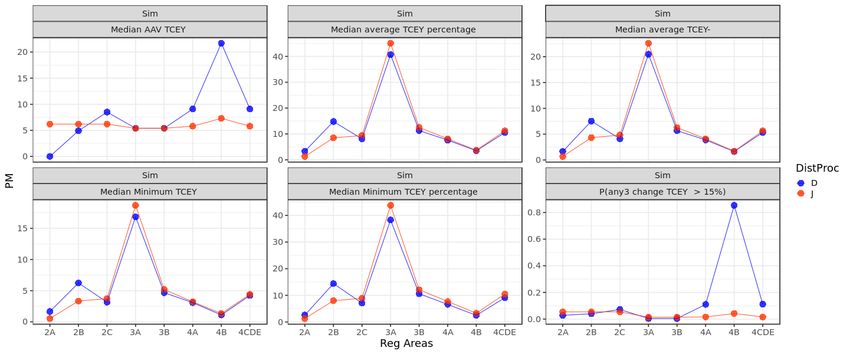
IPHC-2021-AM097-11

Figure 13: Performance metrics by IPHC Regulatory Areas for MPs A through K using simulated
estimation error with an SPR value of 43%. The AAV for TCEY is shown in a). The probability
that the annual change exceeds 15% in 3 or more years is shown in b). The median TCEY with
5th and 95th quantiles is shown in c). The median percentage of the TCEY in each IPHC
Regulatory Area is shown in d).

 Page 25 of 49

IPHC-2021-AM097-11

Table 6: Long-term spawning biomass performance metrics by Biological Region and TCEY (Mlbs) short-term performance
metrics by IPHC Regulatory Areas for MPs A through K with an SPR value of 43% using simulated estimation error.
 Input SPR/TM 43% 43% 43% 43% 43% 43% 43% 43% 43% 43% 43%
 Distribution Procedure A B C D E F G H I J K
 Number of Simulations 500 500 500 500 500 500 500 500 500 500 500
 Biological Sustainability
 P(%SBR=2 < 5%)

IPHC-2021-AM097-11

Table 7: Percentage of TCEY (Mlbs) short-term performance metrics by IPHC Regulatory Areas for MPs A through K with
an SPR value of 43% using simulated estimation error.
 Input SPR/TM 43% 43% 43% 43% 43% 43% 43% 43% 43% 43% 43%
 Distribution Procedure A B C D E F G H I J K
 Number of Simulations 500 500 500 500 500 500 500 500 500 500 500
 Fishery Sustainability
 Median Minimum % TCEY 2A 2.9% 3.4% 3.4% 3.3% 3.4% 1.0% 1.3% 1.2% 1.4% 1.4% 1.3%
 Median Minimum % TCEY 2B 16.1% 16.2% 16.1% 14.5% 7.6% 20.0% 8.0% 7.5% 9.1% 8.5% 7.9%
 Median Minimum % TCEY 2C 6.9% 7.2% 6.9% 7.5% 8.5% 7.2% 8.9% 8.3% 9.7% 9.5% 8.8%
 Median Minimum % TCEY 3A 37.9% 39.2% 37.4% 40.4% 42.8% 39.4% 44.4% 40.8% 40.4% 45.1% 39.8%
 Median Minimum % TCEY 3B 10.5% 10.9% 13.8% 11.2% 11.9% 10.9% 12.3% 15.1% 13.6% 12.5% 14.7%
 Median Minimum % TCEY 4A 4.9% 5.0% 4.8% 5.1% 5.4% 5.0% 5.6% 6.5% 5.4% 6.0% 6.9%
 Median Minimum % TCEY 4CDE 6.9% 6.9% 6.7% 7.0% 7.5% 6.9% 7.7% 8.9% 8.1% 8.3% 9.5%
 Median Minimum % TCEY 4B 2.5% 2.8% 2.7% 3.0% 3.1% 2.8% 3.2% 2.9% 3.2% 3.9% 4.5%

 Median average % TCEY 2A 4.4% 4.5% 4.5% 4.2% 4.5% 1.2% 1.4% 1.3% 1.6% 1.4% 1.3%
 Median average % TCEY 2B 16.4% 16.5% 16.4% 14.8% 8.4% 20.0% 8.9% 8.3% 10.1% 9.0% 8.3%
 Median average % TCEY 2C 8.0% 8.1% 7.8% 8.5% 9.4% 8.2% 9.9% 9.2% 10.8% 10.0% 9.2%
 Median average % TCEY 3A 41.2% 41.4% 39.4% 42.6% 45.4% 41.5% 46.9% 43.2% 42.9% 46.7% 41.5%
 Median average % TCEY 3B 11.4% 11.5% 14.6% 11.8% 12.6% 11.5% 13.0% 16.0% 14.5% 12.9% 15.4%
 Median average % TCEY 4A 5.6% 5.7% 5.5% 5.9% 6.2% 5.7% 6.4% 7.5% 6.2% 6.4% 7.7%
 Median average % TCEY 4CDE 8.3% 8.0% 7.7% 8.0% 8.6% 8.0% 8.9% 10.3% 9.3% 8.9% 10.7%
 Median average % TCEY 4B 3.7% 3.9% 3.8% 4.1% 4.3% 3.9% 4.4% 4.1% 4.6% 4.5% 5.6%

 Page 27 of 49

IPHC-2021-AM097-11

Table 8: Short-term fishery stability performance metrics by IPHC Regulatory Areas for MPs A through K with an SPR value
of 43% using simulated estimation error.
 Input SPR/TM 43% 43% 43% 43% 43% 43% 43% 43% 43% 43% 43%
 Distribution Procedure A B C D E F G H I J K
 Number of Simulations 500 500 500 500 500 500 500 500 500 500 500
 Fishery Sustainability
 P(any3 change TCEY 2A > 15%) 0.01 0.00* 0.00* 0.00* 0.00* 0.38 0.33 0.32 0.30 0.29 0.04
 P(any3 change TCEY 2B > 15%) 0.28 0.27 0.28 0.06 0.41 0.10 0.33 0.32 0.30 0.29 0.04
 P(any3 change TCEY 2C > 15%) 0.46 0.41 0.42 0.11 0.41 0.38 0.33 0.32 0.30 0.29 0.04
 P(any3 change TCEY 3A > 15%) 0.34 0.40 0.40 0.06 0.39 0.32 0.31 0.30 0.30 0.29 0.04
 P(any3 change TCEY 3B > 15%) 0.34 0.40 0.40 0.06 0.39 0.32 0.30 0.30 0.30 0.29 0.04
 P(any3 change TCEY 4A > 15%) 0.52 0.48 0.48 0.19 0.46 0.43 0.40 0.38 0.45 0.31 0.50
 P(any3 change TCEY 4CDE > 15%) 0.50 0.48 0.49 0.21 0.47 0.42 0.42 0.38 0.43 0.29 0.50
 P(any3 change TCEY 4B > 15%) 0.94 0.92 0.91 0.90 0.92 0.92 0.91 0.91 0.93 0.34 0.48

 Median AAV TCEY 2A 0.0% 0.0% 0.0% 0.0% 0.0% 11.2% 10.8% 10.7% 10.8% 9.6% 9.8%
 Median AAV TCEY 2B 12.2% 9.4% 9.4% 6.5% 11.1% 9.5% 10.8% 10.8% 10.8% 9.6% 9.8%
 Median AAV TCEY 2C 15.3% 11.5% 11.5% 9.1% 11.1% 11.2% 10.8% 10.8% 10.8% 9.6% 9.8%
 Median AAV TCEY 3A 13.2% 10.2% 10.1% 6.8% 10.1% 9.7% 9.8% 9.9% 9.7% 9.4% 9.7%
 Median AAV TCEY 3B 13.2% 10.2% 10.1% 6.8% 10.1% 9.7% 9.8% 9.9% 9.7% 9.4% 9.7%
 Median AAV TCEY 4A 16.1% 12.5% 12.5% 10.2% 12.3% 12.2% 12.1% 12.0% 12.5% 9.6% 9.8%
 Median AAV TCEY 4CDE 14.4% 12.4% 12.5% 10.4% 12.3% 12.1% 12.1% 12.0% 12.4% 9.6% 9.8%
 Median AAV TCEY 4B 28.4% 23.7% 23.6% 22.4% 23.6% 23.4% 23.5% 23.5% 22.6% 10.8% 12.6%
 *These probabilities are zero because by definition the TCEY is fixed at 1.65 Mlbs in IPHC Regulatory Area 2A for these MPs.

 Page 28 of 49

IPHC-2021-AM097-11

Table 9: Long-term performance metrics for biological sustainability objectives for MPs A through K with an SPR value of
43% using simulated estimation error. Red shading indicates that the currently defined objective is not met, and green
shading indicates that the objective is met. Values in the cells are the calculated probabilities.

 Performance
 Objective A B C D E F G H I J K
 Metric

 Maintain a coastwide
 female SB above a
 P(SB < SBLim) 0.00 0.00 0.00 0.01 0.00 0.00 0.00 0.00 0.00 0.00 0.00
 biomass limit reference
 point 95% of the time

 Maintain a minimum
 P(%SBR=2 < 5%) 0.00 0.00 0.00 0.01 0.00 0.00 0.00 0.00 0.00 0.00 0.00
 proportion of female SB

 Maintain a minimum
 P(%SBR=3 < 33%) 0.00 0.00 0.00 0.01 0.00 0.00 0.00 0.00 0.00 0.00 0.00
 proportion of female SB

 Maintain a minimum
 P(%SBR=4 < 10%) 0.00 0.00 0.00 0.01 0.00 0.00 0.00 0.00 0.00 0.00 0.00
 proportion of female SB

 Maintain a minimum
 P(%SBR=4B < 2%) 0.15 0.15 0.15 0.15 0.15 0.15 0.16 0.15 0.16 0.16 0.18
 proportion of female SB

Table 10: Long-term performance metrics for fishery objective 2.1 for MPs A through K with an SPR value of 43% using
simulated estimation error. The ranks are determined by how close the long-term probability is to 0.5 after rounding to two
decimal places. Blue shading represents the ranking with light coloring indicating the objective is better met compared to
other management procedures.

 Objective Performance Metric A B C D E F G H I J K

 Maintain the coastwide
 female SB above a target P(SB < SB36%) 11 4 4 1 4 4 4 2 2 4 4
 at least 50% of the time

 Page 29 of 49

IPHC-2021-AM097-11

Figure 14: Distribution of the percentage of spawning biomass in each Biological Region after
60 years of projections with no fishing mortality. The right panel is zoomed in on Biological
Region 4B. A horizontal line shows the 5% quantile in each plot. Primary objectives are to
maintain the female spawning biomass above 5%, 33%, 10%, and 2% for Biological Regions 2,
3, 4, and 4B, respectively. These limits are shown in orange horizontal lines.

The ranking of short-term performance metrics for the Fishery Sustainability objectives are
shown in Table 10, Table 11, Table 12, and Table 13. Higher ranks generally occurred for MPs
D, I, J, and K, although not necessarily for IPHC Regulatory Areas 2A and 2B when compared
to MPs where agreements for those areas are in place. The general objectives were averaged
over IPHC Regulatory Areas to produce a summary of ranks as shown in Table 14. This
summary shows that MPs D and J generally have higher ranks for stability and yield objectives
specific to IPHC Regulatory Areas, although better stability at the IPHC Regulatory Area level
does not imply stability at the coastwide level. Further summarizing the ranks to general
objectives are shown in Table 15, with better averaged performance for MPs D, I, J, and K, in
general.

 Page 30 of 49

IPHC-2021-AM097-11

 Table 11: Short-term performance metrics for fishery stability objectives for MPs A through K
 with an SPR value of 43% using simulated estimation error. Blue shading represents the ranking
 with light coloring indicating the objective is better met compared to other management
 procedures. Ranks were determined after rounding probabilities (i.e. P(AC3>15%)) to two
 decimals and percentages (i.e. AAV) to one decimal.
Objective Performance Metric A B C D E F G H I J K
Limit TCEY AC P(AC3 > 15%) 11 1 1 10 1 1 1 1 1 1 1
Limit TCEY AAV Median AAV TCEY 11 3 2 1 3 8 8 3 3 8 3
 P(AC3 2A > 15%) 5 1 1 1 1 11 10 9 8 7 6
 Limit AC in Reg

 P(AC3 2B > 15%) 5 4 5 2 11 3 10 9 8 7 1
 Areas TCEY

 P(AC3 2C > 15%) 11 8 10 2 8 7 6 5 4 3 1
 P(AC3 3A > 15%) 8 10 10 2 9 7 6 4 4 3 1
 P(AC3 3B > 15%) 8 10 10 2 9 7 4 4 4 3 1
 P(AC3 4A > 15%) 11 8 8 1 7 5 4 3 6 2 10
 P(AC3 4CDE > 15%) 10 8 9 1 7 4 4 3 6 2 10
 P(AC3 4B > 15%) 11 7 4 3 7 7 4 4 10 1 2
 Median AAV 2A 1 1 1 1 1 11 9 8 9 6 7
 Limit AAV in Reg

 Median AAV 2B 11 2 2 1 10 4 7 7 7 5 6
 Areas TCEY

 Median AAV 2C 11 9 9 1 7 8 4 4 4 2 3
 Median AAV 3A 11 10 8 1 8 3 6 7 3 2 3
 Median AAV 3B 11 10 8 1 8 3 6 7 3 2 3
 Median AAV 4A 11 8 8 3 7 6 5 4 8 1 2
 Median AAV 4CDE 11 8 10 3 7 5 5 4 8 1 2
 Median AAV 4B 11 10 8 3 8 5 6 6 4 1 2

 Table 12: Short-term performance metrics for fishery yield objectives related to the TCEY for
 MPs A through K with an SPR value of 43% using simulated estimation error. Blue shading
 represents the ranking with light coloring indicating the objective is better met compared to other
 management procedures. Ranks were determined after rounding to the nearest one million
 pounds.
Objective Performance Metric A B C D E F G H I J K
Optimize
 Median TCEY 1 3 3 1 3 3 3 3 3 3 3
TCEY
 Median Min 2A 1 1 1 1 1 6 6 6 6 6 6
 minimum TCEY

 Median Min 2B 5 2 2 2 8 1 8 8 6 6 8
 by Reg Areas

 Median Min 2C 8 8 8 1 1 8 1 1 1 1 1
 Maintain

 Median Min 3A 11 5 10 1 2 5 2 5 5 2 5
 Median Min 3B 9 9 2 2 2 9 2 1 2 2 2
 Median Min 4A 11 1 1 1 1 1 1 1 1 1 1
 Median Min 4CDE 5 5 5 5 5 5 5 1 1 1 1
 Median Min 4B 1 1 1 1 1 1 1 1 1 1 1
 Optimize Reg Areas

 Median TCEY 2A 1 1 1 1 1 9 6 9 6 6 9
 Median TCEY 2B 2 3 3 3 7 1 7 7 6 7 7
 Median TCEY 2C 5 5 5 5 1 5 1 5 1 1 5
 TCEY

 Median TCEY 3A 3 6 11 3 3 6 1 6 6 1 6
 Median TCEY 3B 5 10 1 5 5 10 5 1 1 5 1
 Median TCEY 4A 3 3 3 3 3 3 3 1 3 3 1
 Median TCEY 4CDE 4 4 4 4 4 4 4 1 1 4 1
 Median TCEY 4B 6 6 6 1 6 6 1 6 1 1 1

 Page 31 of 49

IPHC-2021-AM097-11

Table 13: Short-term performance metrics for fishery yield objectives related to the percentage
of TCEY in each IPHC Regulatory Area for MPs A through K with an SPR value of 43% using
simulated estimation error. Blue shading represents the ranking with light coloring indicating the
objective is better met compared to other management procedures. Ranks were determined
after rounding to two decimals.
Objective Performance Metric A B C D E F G H I J K
 Median Min % 2A 5 1 1 4 1 11 8 10 6 6 8
 Median Min % 2B 3 2 3 5 10 1 8 11 6 7 9
 TCEY by Reg
 minimum %

 Median Min % 2C 10 8 10 7 5 8 3 6 1 2 4
 Maintain

 Areas

 Median Min % 3A 10 9 11 5 3 8 2 4 5 1 7
 Median Min % 3B 11 9 3 8 7 9 6 1 4 5 2
 Median Min % 4A 10 8 11 7 5 8 4 2 5 3 1
 Median Min % 4CDE 8 8 11 7 6 8 5 2 4 3 1
 Median Min % 4B 11 8 10 6 5 8 3 7 3 2 1
 Median % TCEY 2A 4 1 1 5 1 11 7 9 6 7 9
 among Reg Areas
 Optimize TCEY

 Median % TCEY 2B 3 2 3 5 9 1 8 10 6 7 10
 percentage

 Median % TCEY 2C 10 9 11 7 4 8 3 5 1 2 5
 Median % TCEY 3A 10 9 11 6 3 7 1 4 5 2 7
 Median % TCEY 3B 11 9 3 8 7 9 5 1 4 6 2
 Median % TCEY 4A 10 8 11 7 5 8 3 2 5 3 1
 Median % TCEY 4CDE 7 8 11 8 6 8 4 2 3 4 1
 Median % TCEY 4B 11 8 10 6 5 8 4 6 2 3 1

 Page 32 of 49