Comparison of Acoustic to Optical Backscatter Continuous Measurements of Suspended Sediment Concentrations and Their Characterization in an ...
←
→
Page content transcription
If your browser does not render page correctly, please read the page content below

water
Article
Comparison of Acoustic to Optical Backscatter
Continuous Measurements of Suspended Sediment
Concentrations and Their Characterization in
an Agriculturally Impacted River
Zacharie Sirabahenda 1, * , André St-Hilaire 1 , Simon C. Courtenay 2 and
Michael R. van den Heuvel 3
 1   Canadian Rivers Institute, INRS-ETE, 490 Rue de la Couronne, Québec City, QC G1K 9A9, Canada;
     Andre.St-Hilaire@ete.inrs.ca
 2   Canadian Rivers Institute, School of Environment, Resources and Sustainability, University of Waterloo,
     200 University Avenue West, Waterloo, ON N2L 3G1, Canada; scourten@connect.uwaterloo.ca
 3   Canadian Rivers Institute, Department of Biology, University of Prince Edward Island,
     550 University Avenue, Charlottetown, PEI C1A 4P3, Canada; mheuvel@upei.ca
 *   Correspondence: zacharie.sirabahenda@ete.inrs.ca

 Received: 19 March 2019; Accepted: 8 May 2019; Published: 10 May 2019

 Abstract: The increased soil loss in an agricultural watershed raises challengers for river water quality
 and a reliable automated monitoring for suspended sediment concentrations (SSC) is crucial to
 evaluate sediment budgets variation in systems. The aims of this study were (1) to test if an acoustic
 doppler current profiler (ADCP) would give similar results to turbidity probe measurements as a high
 frequency monitoring tool for suspended sediment; and (2) to analyze the relationship between
 sediment drivers and SSC in a typical agricultural drainage basin. The acoustic and optical backscatter
 sensors were used to collect SSC data during the ice-free seasons of four consecutive years in the Dunk
 River (PEI, Canada). The slopes of the relationships between the two SSC indirect measurements
 were not significantly different than 1. Correlations between SSC and hydro-meteorological variables
 showed that the high SSC values were more associated with the streamflow and water velocity than
 precipitation. This study highlighted the great potential of ADCP for the continuous monitoring
 of suspended sediment in an agricultural watershed. For summer periods the prevalence of
 clockwise hysteresis (74.1% of measured rainstorm events with SSC > 25 mg L−1 ) appeared related to
 rainstorm behaviors.

 Keywords: turbidity; ADCP; sediment dynamic; agricultural watershed

1. Introduction
     River water quality and ecosystem integrity are often threatened by human activities [1,2]. Rivers
within agricultural watersheds can be impacted by erosion that leads to a high level of turbidity and
an increase of the sediment-associated pollutant load originating from the drainage basin. This in
turn, may result in damage to aquatic flora and fauna [3,4]. The increased soil loss rate in farm
fields raises challenges for implementing soil conservation techniques [5,6]. Water resource protection
strategies need to include in situ measurement protocols for detecting changes in suspended sediment
concentration (SSC) in order to evaluate remedial actions.
     A cost-effective and reliable automated sampling or monitoring strategy for SSC is essential to
develop sediment budgets in systems. Optical backscatter sensors (OBS), and more recently acoustic
backscatter sensors, are indirect SSC monitoring techniques suitable for continual monitoring that

Water 2019, 11, 981; doi:10.3390/w11050981                                         www.mdpi.com/journal/water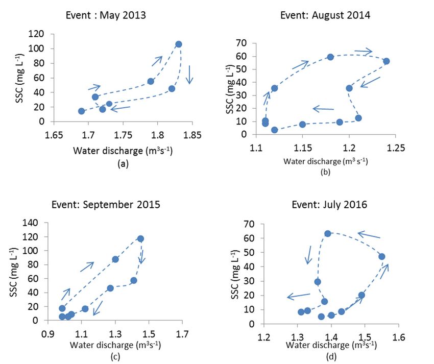
Water 2019, 11, 981                                                                                   2 of 12

is essential for a highly temporally variable such as SSC [7–9]. The technologies of both types of
instrument have improved markedly recently and they have been successfully applied to quantifying
the suspended sediment transports in many fluvial environments [10–14]. The more recently introduced
ADCPs have the advantage of being able to collect vertical profiling of sediment concentration and
water velocity variation as compared to OBS. Furthermore, the conversion of backscatter data to SSC is
complicated due to the site-specific variability in sediment physical properties [15,16]. Co-deployment
of optical and acoustic backscatter sensors is one option that allows for partial validation of site-specific
calibration [17–20].
       Investigations over recent decades show an increasing interest in links between the drivers of
suspended sediment transport in rivers and the uncertainties related to their spatial and temporal
variability [21–23]. Hydro-climatic factors, in interaction with catchment characteristics, have been
identified as the dominant drivers for suspended sediment loading over many time scales [24–26].
However, sediment budget variation was found to be strongly dependent on local conditions and there
is still need of a better understanding of the functional relationships between variables that most affect
sediment dynamics. Hence, a systematic assessment of the degree of correlation and hysteresis patterns
between hydro-climatic factors and SSC provides valuable insights for development of sediment
estimation tools within rivers [27,28].
       Environmental stakeholders in Prince Edward Island (PEI) recognize the increasing degradation
of the water quality in estuaries and coastal waters. Sediments from intense agricultural activities
are among the major sources of pollution [16,29]. The soils in PEI are extremely sensitive to water
erosion and the soil losses have been reported as a major long-term environmental and economic
challenge for the province [30,31]. The Dunk River (PEI, Canada) has historically experienced fish
kills linked to the use of pesticides that can bind to soil and/or be transported by erosion processes
on its highly agricultural watershed during summer rainstorms [32,33]. Degradation of its water
quality through high sediment loads caused by an annual mean soil loss estimated at 10 tonnes ha−1
has been reported for over a decade [1,34]. Hence, continuously monitoring suspended sediment
yield, with adequate techniques to acquire representative data, is necessary to support water resources
managers and farm owners in their efforts to address the water quality issues in the Dunk River.
Furthermore, a descriptive analysis focusing on the interdependence between suspended sediment
fluxes and other hydro-meteorological variables may prove instructive in the development of strategies
to protect and preserve its water resources.
       The hypothesis of this study was that the use of ADCP would give similar results to turbidity
probe measurements as a high frequency monitoring tool for suspended sediment in an agricultural
river basin. The hypothesis was examined through continuously monitoring suspended sediment
yield using both technologies in the Dunk River. Furthermore, as a second objective, this study sought
to elucidate descriptive relationships between suspended sediment fluxes and hydro-meteorological
variables. Specifically, the degree of correlation between SSC and the hydro-meteorological variables
was quantified using ADCP backscatter data. The SSC temporal variability was also investigated by
analyzing the hysteresis loops between streamflow and SSC for rainstorm events for different years.

2. Materials and Methods

2.1. Site Description and Instrument Setup
      The Dunk River is situated in the central portion of Prince Edward Island (Canada) and flows into
the Bedeque Bay that empties into the Northumberland Strait in the Southern Gulf of St. Lawrence
(Figure 1). Suspended sediment was measured within the Dunk River at a monitoring station
(46◦ 200 5” N, 63◦ 390 46” W) with an upstream watershed surface area of 140.6 km2 . The studied
watershed area is dominated by agriculture (66.1%) while the forest covers an area of 25.1%.
The topographic relief is largely of moderately undulating plains with low slopes [1]. The Dunk
watershed soils are geologically derived from sedimentary rocks known as redbeds and formed during
Water 2019, 11, x FOR PEER REVIEW 3 of 12
Water 2019, 11, 981 3 of 12
are the Charlottetown soil series (mainly well drained) and the Albery soil series (moderately
drained) occupying, respectively, 74.4% and 17.7% of the total surface area.
the Stephanian-late Early Permian period [35]. The two dominant soil types for the study area are
the Charlottetown soil series (mainly well drained) and the Albery soil series (moderately drained)
occupying, respectively, 74.4% and 17.7% of the total surface area.
Figure 1. Dunk River Watershed location.
Figure 1. Dunk River Watershed location.
SSCs data were collected using acoustic and optical instruments during monitoring campaigns in
May–August
SSCs data2013, andcollected
were from June untilacoustic
using Octoberand
for the yearsinstruments
optical 2014–2016. A Sentinel
during V-ADCP campaigns
monitoring (1000 KHz
with four beams) from Teledyne RD Instruments (Poway, CA, USA) was
in May–August 2013, and from June until October for the years 2014–2016. A Sentinel V-ADCPdeployed on the river(1000
bed
(upward-looking) for acoustic backscatter monitoring (minimum depth above
KHz with four beams) from Teledyne RD Instruments (Poway, CA, USA) was deployed on the river the ADCP: 0.95 m).
Itbed
was(upward-looking)
set up to collect velocity and acoustic
for acoustic backscatter
backscatter in 1 min
monitoring bursts (60depth
(minimum pings)above
every 30
themin.
ADCP:The 0.95
bin
size and the blank distance were configured to 0.30 m and 0.30 m, respectively. To avoid
m). It was set up to collect velocity and acoustic backscatter in 1 min bursts (60 pings) every 30 min. any errors
due
Thetobinmagnetic
size andfield distortions,
the blank the were
distance compass calibration
configured wasm
to 0.30 first
and conducted at the monitoring
0.30 m, respectively. station
To avoid any
location as per manufacturer’s instructions.
errors due to magnetic field distortions, the compass calibration was first conducted at the monitoring
Forlocation
station optical as
backscatter sampling,instructions.
per manufacturer’s a YSI 6136 turbidity probe from Teledyne RD Instruments
(Poway,ForCA, USA)
optical was installed
backscatter near the
sampling, Sentinel
a YSI 6136 V for sampling
turbidity probe turbidity data inRD
from Teledyne nephelometric
Instruments
turbidity units (NTU) with a recording frequency of 30 min during the same
(Poway, CA, USA) was installed near the Sentinel V for sampling turbidity data in nephelometricperiod. The turbidity
measured by the(NTU)
turbidity units YSI sensor
with aare based onfrequency
recording the absorption
of 30 of
min infrared
duringradiation
the sameemitted
period. by
Thethe sensor
turbidity
and backscattered
measured by suspended
by the YSI sediment
sensor are based through
on the the water
absorption body [36].
of infrared YSI-certified
radiation emittedpolymer-based
by the sensorWater 2019, 11, 981 4 of 12
standards were used for primary calibration and the unit associated with turbidity readings was NTU.
For the proper device maintenance and to avoid bio-fouling effects, a regular daily automatic cleaning
was set up and an instrument calibration was completed every year.
2.2. Conversion of the Acoustic and Optical Backscatters Data to SSC
The relationship between the turbidity measurements in NTU and SSC in mg L−1 was determined
using sediment concentrations of the mixtures of in situ water and local sediment as a function of
their correspondent recorded turbidity. Local water and sediments (wet sieved using a 63-µm sieve to
retain only the fine particles that are most likely to be suspended in the water column) were mixed
at different concentrations in a 40 L container and mixed constantly while the turbidity meter was
immersed in the solution. This protocol was repeated many times to cover the largest possible range
of SSC values [37]. The sediment concentrations of the grab samples were calculated after filtering,
drying, and weighing in the laboratory. Thus, data were fitted with a non-linear function (Equation (1))
using the Levenberg-Marquardt algorithm, using the nlinfit function in Matlab software developed by
The Mathworks, Inc. (Natick, MA, USA) [38]:
SSC = a1 × (Turbidity)b1 (1)
where SSC and Turbidity are expressed in mg L−1 and in NTU, respectively; a1 and b1 are coefficients to
be estimated.
Backscatter data recorded by the Sentinel V-ADCP were calibrated against concentration of
sediment in collocated grab samples. To cover a wide range of sediment concentrations encountered
in river, solutions with different concentrations were pumped gradually upstream of the Sentinel V
and were allowed to flow downstream. Grab samples associated with different SSC were collected
above the ADCP concomitantly with V-ADCP measurements. For the conversion of the received echo
intensity to SSC, the exponential form of the sonar equation [39] was used:
10 log10 (SSC) = a2 + b2 Idb (2)
where a2 and b2 are parameters representing the characteristics of the instrument obtained by calibration
using a linear regression analysis; Idb is the relative acoustic backscatter and expressed based on the
equation proposed by Deinnes [40]:
Idb = C + 10 log10 ((T + 273.16)R2 ) − 10 log10 (Lt ) − 10 log10 (Pw ) + 2αR + Kc (E − Er ) (3)
D
R = r+ (4)
4
where C is a constant combining several parameters specific to each instrument, T is the temperature
measured at the transducer (◦ C); R is the slant distance (m); r is the distance between the surface of
the sentinel V-ADCP emitters and the midpoint of the bin (m); D is the width of the bin (m); Lt is
the transmit pulse length (m); Pw is the acoustic transmit power level (w); α represent the absorption
coefficient combining the sound absorption factor due to water αw and the sound absorption by
particles αs due to properties of sediment; E is the received signal strength indicator (RSSI) amplitude
for each bin recorded by the Sentinel V-ADCP (counts); Er is the RSSI amplitude in the absence of noise
(counts) and it is calibrated to be 40 counts for the Sentinel V-ADCP [41]; Kc is a conversion factor for
counts to decibels and it calibrated to be 0.40 db count−1 for the Sentinel V-ADCP [41].
Inter-annual correspondence of SSC estimated by acoustic backscatter versus optical backscatter
was quantified using four commonly used index statistics [42]: the Nash-Sutcliffe efficiency (NSE),
the Coefficient of determination (R2 ), the root mean square error (RMSE) and the percent bias (PBIAS).
The NSE is a standardized statistic that indicates the relative magnitude of the residual variance
compared to the measured data variance [43]. The NSE is calculated with Equation (5) and can rangeWater 2019, 11, 981 5 of 12
from −∞ to 1. The values of NSE close to 1 indicate a high level of performance for a model. The RMSE
indicates the error in the units of the variable of interest. The R2 describes the degree of collinearity
between two variables data while the PBIAS measures the average absolute difference between the
two methods [44]. The PBIAS is computed as shown in Equation (6) and a good model is characterized
by the low values of PBIAS. The R2 is similar to NSE and its values ranges between 0 (the model
explains no variance) and 1 (perfect linear relationship between model and measurements). The RMSE
indicates the error in the units of the variable of interest. It is calculated with Equation (7) and values
close to 0 indicate a good agreement between observed values and predicted values:
(Xi − Yi )2
Pn
NSE = 1 − P i=1 2
(5)
n
i = 1 ( Xi − X i )
Pn
i=1 (Xi − Yi ) × 100
PBIAS = Pn (6)
i = 1 Xi
s
(Xi − Yi )2
Pn
i=1
RMSE = (7)
n
where Xi and Xi are, respectively, the observed data and their average, n is the number of observations
and Yi refers to the simulated data by a model.
2.3. Characterization of Sediment Temporal Variation
The SSCs from acoustic backscatter data were used to characterize the catchment’s sediment
dynamic in relation to the hydro-climatic factors precipitation, streamflow and water velocity. The daily
precipitation data for Elmwood and New Glasgow stations (http://climate.weather.gc.ca) and daily
water discharges for Dunk River at Wall Road station (https://wateroffice.ec.gc.ca) operated by
Environment and Climate Change Canada were used. Its interannual average discharge is 2.55 m3 s−1
while the highest and lowest daily averages are respectively equal to 0.212 m3 s−1 and 84.7 m3 s−1 .
The Climate Normals (1981–2010) indicate that the total annual precipitation is on average 1257.9 mm
(944.3 mm for rainfall and 313.6 mm for snow). The extreme daily total rainfall was 85.6 mm and the
maximum number of days with rainfall ≥10 mm was 29.7 for the New Glasgow station.
The two most commonly used correlation coefficients (Pearson coefficient and Spearman
coefficient [45]) were retained to see how well the variables related. Those correlation measurements
between data sets were chosen because linear and non-linear relationships are both possible between
hydro-climatic factors and SSC. Pearson’s r correlation is used to measure the degree of the relationship
between linearly related variables. Spearman’s rank correlation is a non-parametric test that is used to
assess the strength of the monotonic association between two variables [46]. Hence, the sensitivity
analysis was made by calculating those indices of correlation for four subsets data: SSC > 25 mg L−1 ,
SSC > 15 mg L−1 , SSC > 10 mg L−1 and SSC > 0 mg L−1 . The temporal sediment loading patterns were
explored by quantifying of the number of rainfall events displaying clockwise versus anti-clockwise
hysteresis loops between SSC and streamflow.
3. Results
3.1. Indirect Suspended Sediment Measurements
For the OBS, the non-linear relationship between the SSC in mg L−1 as a function of the turbidity
in NTU (i.e., the calibration curve) is presented in Figure 2 (NSE and R2 = 0.96 and 0.95, respectively).
Figure 3 shows the suspended sediment calibration curve for the ADCP that resulted from the
linear regression analysis (R2 = 0.90 with p < 0.001 for 10 log10 (SSC) as a function of intensity of
echo backscatter).Water2019,
Water 2019,11,
11,981
x FOR PEER REVIEW 66ofof1212
Water 2019, 11, x FOR PEER REVIEW 6 of 12
Figure 2. Suspended sediment calibration curve for a turbidity probe YSI 6136.
Figure2.2.Suspended
Figure Suspendedsediment
sedimentcalibration
calibrationcurve
curvefor
foraaturbidity
turbidityprobe
probeYSI
YSI6136.
6136.
) )
-1
(SSC)
loglog(SSC)
10
L -1L
(mg(mg
10
10 10
Figure 3. 3.
Figure Suspended sediment
Suspended calibration
sediment curve
calibration forfor
curve thethe
Sentinel V-ADCP.
Sentinel V-ADCP.
Figure 3. Suspended sediment calibration curve for the Sentinel V-ADCP.
The
Theslope
slopeofofthe
therelationship
relationshipbetween
betweenSSCSSCasasdetermined
determinedby byADCP
ADCPvs. vs.that
thatdetermined
determinedusing using
The
turbidity slope
turbiditywas
was0.9, of the
0.9,0.87, relationship
0.87,0.85,
0.85,and
and0.87 between
0.87for
forthe SSC
thefour as determined
fouryears
yearsexamined. by
examined.WhileADCP
Whilethis vs. that
thisindicatesdetermined
indicates that
thatthe using
theADCP
ADCP
turbidity slightly
produced
produced was 0.9,lower
slightly 0.87,
lower0.85, andthese
values,
values, 0.87
thesefor thewere
slopes
slopesfour years
werenot examined.
significantly
not While thisthan
different
significantly different indicates that
1 (Table
than 1 (Table1, the ADCP
Figure 4).
1, Figure
produced
Despite a slightly
significant lower values,
agreement these
betweenslopes
the were
two not significantly
measurement different
approaches, than
the
4). Despite a significant agreement between the two measurement approaches, the acoustic method 1 (Table
acoustic 1, Figure
method
4). Despite
provided
provided a significant
generally
generally lower
lower agreement
values
valuesthan between
thanoptical the two for
opticalmethod
method measurement
forhigh approaches,
highsediment
sediment the acoustic
concentrations
concentrations (Figure
(Figuremethod
4).4).
provided generally lower values than optical method for high sediment concentrations (Figure 4).Water 2019, 11, 981 7 of 12
Table 1. Statistics for acoustic backscattered versus optical backscattered data.
Water 2019, 11, x FOR PEER REVIEW 7 of 12
n NSE R2 p RMSE PBIAS
Annual
Table Period for acoustic backscattered versus optical backscattered data.
1. Statistics
(Days) (mg L−1 ) (%)
17 May–27 to n NSE R2 p RMSE PBIAS
Annual Period 103 0.96 0.98Water 2019, 11, 981 8 of 12
Water 2019,Table 2. Significant
11, x FOR PEER REVIEW correlation (p < 0.05%) for Spearman (Rho) and Pearson (r). 8 of 12
SSC—Flow
Table 2. Significant correlation (p < 0.05%)SSC—Precipitation
for Spearman (Rho) andSSC—Velocity
Pearson (r).
Threshold of SSC
Rho r Rho r Rho r
SSC—Flow SSC—Precipitation SSC—Velocity
Threshold of SSC2013 0.58
Rho 0.49 r 0.33
Rho 0.23
r 0.60
Rho r0.54
20142013 0.30 0.30 0.44 0.33 0.23 0.26
SSC > 0 mg L −1 0.58 0.49 0.33 0.23 0.60 0.54
2015 0.39 0.17 0.46 0.62
2014 0.30 0.30 0.44 0.33 0.23 0.26
SSC > 0 mg L−12016 0.26 0.34 0.43 0.41 0.23 0.21
2015 0.39 0.17 0.46 0.62
20132016 0.340.26 0.280.34 0.29
0.43 0.25
0.41 0.40
0.23 0.43
0.21
2014 0.22
2013 0.34 0.28 0.21 −0.41
0.29 −0.35
0.25 0.40 0.29
0.43
SSC > 10 mg L−1
2015 0.20 0.25 0.43 0.29 0.23 0.15
2014 0.22 0.21 −0.41 −0.35 0.29
SSC > 10 mg L−1 2016 0.23 0.30 0.43 0.28 0.35
2015 0.20 0.25 0.43 0.29 0.23 0.15
20132016 0.450.23 0.300.30 0.34
0.43 0.37 0.49
0.28 0.52
0.35
20142013 0.340.45 0.27
0.30 −0.33
0.34 0.21
0.37 0.40
0.49 0.37
0.52
SSC > 15 mg L −1
20152014 0.350.34 0.31
0.27 0.58
−0.33 0.45
0.21 0.39
0.40 0.40
0.37
SSC > 15 mg L−1 2016 0.27 0.30 0.31 0.36 0.38 0.45
2015 0.35 0.31 0.58 0.45 0.39 0.40
20132016 0.510.27 0.540.30 0.21
0.31 0.36 0.61
0.38 0.56
0.45
2014 0.46
2013 0.51 0.54 0.31 −0.17
0.21 0.40
0.61 0.34
0.56
SSC > 25 mg L−1
20152014 0.44 0.19
0.46 0.31 0.41
−0.17 0.55 0.49
0.40 0.36
0.34
SSC > 25 mg L−1 20162015 0.410.44 0.380.19 0.21
0.41 0.37
0.55 0.49
0.49 0.48
0.36
2016 0.41 0.38 0.21 0.37 0.49 0.48
The indices of correlation were moderately weak for precipitation and streamflow and showed
The indices of correlation were moderately weak for precipitation and streamflow and showed
that there were neither high significant linear relationships nor high significant monotonic function
that there were neither high significant linear relationships nor high significant monotonic function
with the SSC. For high SSC (>25 mg L−1 ),−1the indices of correlation were relatively improved for the
with the SSC. For high SSC (>25 mg L ), the indices of correlation were relatively improved for the
streamflow and the water velocity. The hysteresis patterns between SSC and water discharge for events
streamflow and the water velocity. The hysteresis patterns between SSC and water discharge for
with SSC >
events25with L−1 >were
mg SSC analyzed
25 mg L−1 weregraphically and an example
analyzed graphically from each
and an example fromyear is year
each shown in Figure
is shown in 5.
Over all monitoring campaign periods we collected a total of 27 events of which 20 events
Figure 5. Over all monitoring campaign periods we collected a total of 27 events of which 20 events (74.1%)
show clockwise
(74.1%) showhysteresis
clockwiseloops, fourloops,
hysteresis events (14.8%)
four events had anti-clockwise
(14.8%) hysteresis
had anti-clockwise loops
hysteresis andand
loops three
events three events
(11.1%) were (11.1%) were mixed-shaped
mixed-shaped loops. Thisloops. This
result result highlighted
highlighted that thethat the pattern
pattern of SSC–
of SSC–discharge
discharge
relationship relationship
for Dunk Riverfor Dunk River is
is dominated bydominated
clockwisebyhysteresis
clockwise loops.
hysteresis loops.
Figure Figure 5. Typical
5. Typical hysteresis
hysteresis loopsloops observed
observed (daily
(daily averageddata)
averaged data) for
for summers
summersofof2013 (a),(a),
2013 2014 (b),(b),
2014
2015 (c), and 2016
2015 (c), and 2016 (d). (d).Water 2019, 11, 981 9 of 12
4. Discussion
The SSC calculated from data recorded using a sentinel V-ADCP and an YSI 6136 turbidity
probe using established calibration curves did not differ from a slope of 1 for the four studied years.
Their relative high slopes and low y-intercepts of the best-fit regression lines indicated a good agreement
between the two indirect measurement techniques of SSC [47]. However, the acoustic method provided
generally lower values than optical method for high sediment concentrations. The difference may
be due to a slight bias in the acoustic calibration for high of suspended sediment concentrations.
There may also be variations of the particles size distribution for higher vs lower SSC. Moreover,
the trend of SSC underestimation at smaller size distribution conditions by the acoustic method is
often reported in the literature [7,8,17]. Ultimately, the results of this comparison reveal the potential
of the acoustic backscatter technique for a non-intrusive monitoring of SSC within rivers with high
sediment loads. Further investigations are needed for accuracy assessment of the outputs of the two
measurement approaches by in situ automatic sampling during rainstorms events.
The correlation values for streamflow and water velocity increased with an increasing threshold
for SSC. It appears therefore that high SSC are more associated with the river processes. Thus, this
highlighted the important role of the water velocity in sediment transport capacity by the river
during events. The sediment transport capacity also depends on the hydraulic and morphological
characteristics of the river [48,49] and it may increase with the increasing of the flow rate [50]. By
contrast, the impact of the variability of precipitation on SSC appears to be more complex and thorough
investigations are needed to better understand sediment process patterns.
Frequent occurrence of clockwise SSC-flow hysteresis patterns was observed. A similar outcome
has been reported in many previous studies and the rapid exhaustion of available sediments was pointed
out as the principal cause of the clockwise hysteresis patterns [26,51,52]. Dunk River, as an important
PEI alluvial river, the rapid sediment mobilization from land near riparian zone by intense rainstorms
and from the bed river by high flow may potentially result in a clockwise hysteresis loop. There is an
increase in turbulence and discharge within a river during rainstorm events. The high turbulence may
result in high sediment concentration from resuspension of the bed sediments, followed by a gradually
decrease of sediment delivery to the river during prolonged rainstorms [53–55]. The sediment
concentration peaks occur before discharge peaks for clockwise hysteresis loops. The counter-clockwise
hysteresis may be the result of late arrival of sediment at the point of measurement and the timing of
the rainfall events or spatial location could explain waves of higher SSC arriving after the flow had
started to decline [53–55]. The hysteresis loop pattern may be linked to the characteristics of the source
sediment as well as to the frequency and intensity of precipitation [24,56,57].
5. Conclusions
This study focused on the comparison of continual SSC monitoring by acoustic and optical
approaches on the Dunk River and the characterization of sediment dynamic variation. The SSC
calculated from data recorded using an ADCP and an OBS using established calibration curves showed
good agreement between the two techniques. High SSC was more correlated to streamflow and water
velocity than precipitation. The SSC-discharge relationship was dominated by clockwise hysteresis
loops and it may be linked to the characteristics of the source sediment as well as to rainstorms
behaviors for summer periods. Further investigations will be needed for better understanding of
SSC dynamic during all periods of the year. For future work, a close analysis of temporal and spatial
rainfall records, from a denser storm event sampling network would be useful to improve dynamic
sediment characterization.
Author Contributions: Conceptualization: Z.S., A.S.-H., S.C.C., and M.R.v.d.H.; formal analysis: Z.S.; funding
acquisition: A.S.-H.; investigation: Z.S.; methodology: Z.S., A.S.-H., S.C.C., and M.R.v.d.H.; supervision:
A.S.-H., S.C.C., and M.R.v.d.H.; validation: A.S.-H., S.C.C., and M.R.v.d.H.; writing—original draft: Z.S.;
writing—review and editing: A.S.-H., S.C.C., and M.R.v.d.H.Water 2019, 11, 981 10 of 12
Funding: This research was funded by the Canadian Water Network and the Department of Fisheries and Oceans
Canada through support of Northumberland Strait Environmental Monitoring Partnership (NorSt-EMP) node of
the Canadian Watershed Research Consortium and through the Scientific Director’s Research Fund (SCC)
Acknowledgments: We owe thanks to Christina Pater for her assistance during field work.
Conflicts of Interest: The authors declare no conflict of interest. The funders had no role in the design of the
study; in the collection, analyses, or interpretation of data; in the writing of the manuscript, or in the decision to
publish the results.
References
1. Cunjak, R.A.; Newbury, R.W. 21—Atlantic Coast Rivers of Canada. In Rivers of North America; Benke, A.C.,
Cushing, C.E., Eds.; Academic Press: Burlington, VT, USA, 2005; pp. 938–980. [CrossRef]
2. Cloern, J.E.; Abreu, P.C.; Carstensen, J.; Chauvaud, L.; Elmgren, R.; Grall, J.; Greening, H.; Johansson, J.O.R.;
Kahru, M.; Sherwood, E.T.; et al. Human activities and climate variability drive fast-paced change across the
world’s estuarine–coastal ecosystems. Glob. Chang. Biol. 2016, 22, 513–529. [CrossRef]
3. Boyd, C.E. Water Quality: An Introduction, 2nd ed.; Springer: New York, NY, USA, 2015.
4. Suedel, B.C.; Lutz, C.H.; Clarke, J.U.; Clarke, D.G. The effects of suspended sediment on walleye (Sander
vitreus) eggs. J. Soils Sediments 2012, 12, 995–1003. [CrossRef]
5. Hudson, N. Soil Conservation: Fully Revised and Updated, 3rd ed.; New India Publishing Agency: New Delhi,
India, 2015; 392p.
6. Pearce, D.; Barbier, E.; Markandya, A. Sustainable Development: Economics and Environment in the Third World;
Routledge: London, UK, 2000.
7. Ghaffari, P.; Azizpour, J.; Noranian, M.; Chegini, V.; Tavakoli, V.; Shah-Hosseini, M. Estimating suspended
sediment concentrations using a broadband ADCP in Mahshahr tidal channel. Ocean Sci. Discuss. 2011, 8,
1601–1630. [CrossRef]
8. Felix, D.; Albayrak, I.; Boes, R.M. Continuous measurement of suspended sediment concentration: Discussion
of four techniques. Measurement 2016, 89, 44–47. [CrossRef]
9. Merten, G.H.; Capel, P.D.; Minella, J.P.G. Effects of suspended sediment concentration and grain size on
three optical turbidity sensors. J. Soils. Sediments 2014, 14, 1235–1241. [CrossRef]
10. Simmons, S.M.; Parsons, D.R.; Best, J.L.; Oberg, K.A.; Czuba, J.A.; Keevil, G.M. An evaluation of the use
of a multibeam echo-sounder for observations of suspended sediment. Appl. Acoust. 2017, 126, 81–90.
[CrossRef]
11. Sahin, C.; Verney, R.; Sheremet, A.; Voulgaris, G. Acoustic backscatter by suspended cohesive sediments:
Field observations, Seine Estuary, France. Cont. Shelf. Res. 2017, 134, 39–51. [CrossRef]
12. Moura, M.G.; Quaresma, V.S.; Bastos, A.C.; Veronez, P. Field observations of SPM using ADV, ADP, and OBS
in a shallow estuarine system with low SPM concentration—Vitória Bay, SE Brazil. Ocean Dyn. 2011, 61,
273–283. [CrossRef]
13. Zhang, W.-x.; Luo, X.-x.; Yang, S.-l. Comparison between measurements of suspended sediment concentration
using ADP and OBS. J. Sediment Res. 2010, 5, 59–65.
14. Wei, X.; Wang, Y.; Yang, Y.; Chen, J.; Gao, J.; Wang, A.; Li, D.; Hu, G. Suspended sediment concentration in
shallow sea: Comparative study of methods. Mar. Geol. Quat. Geol. 2013, 1, 161–170. [CrossRef]
15. Guerrero, M.; Di Federico, V. Suspended sediment assessment by combining sound attenuation and
backscatter measurements–analytical method and experimental validation. Adv. Water Resour. 2018, 113,
167–179. [CrossRef]
16. Alberto, A.; St-Hilaire, A.; Courtenay, S.C.; van den Heuvel, M.R. Monitoring stream sediment loads in
response to agriculture in Prince Edward Island, Canada. Environ. Monit. Assess. 2016, 188, 415. [CrossRef]
17. Guerrero, M.; Rüther, N.; Haun, S.; Baranya, S. A combined use of acoustic and optical devices to investigate
suspended sediment in rivers. Adv. Water Resour. 2017, 102, 1–12. [CrossRef]
18. Hoitink, A.J.F.; Hoekstra, P. Observations of suspended sediment from ADCP and OBS measurements in
a mud-dominated environment. Coastal Eng. 2005, 52, 103–118. [CrossRef]
19. Marttila, H.; Postila, H.; Kløve, B. Calibration of turbidity meter and acoustic doppler velocimetry
(Triton-ADV) for sediment types present in drained peatland headwaters: Focus on particulate organic peat.
River Res. Appl. 2010, 26, 1019–1035. [CrossRef]Water 2019, 11, 981 11 of 12
20. Moore, S.A.; Le Coz, J.; Hurther, D.; Paquier, A. On the application of horizontal ADCPs to suspended
sediment transport surveys in rivers. Cont. Shelf. Res. 2012, 46, 50–63. [CrossRef]
21. Aich, V.; Zimmermann, A.; Elsenbeer, H. Quantification and interpretation of suspended-sediment discharge
hysteresis patterns: How much data do we need? Catena 2014, 122, 120–129. [CrossRef]
22. Fan, X.; Shi, C.; Shao, W.; Zhou, Y. The suspended sediment dynamics in the Inner-Mongolia reaches of the
upper Yellow River. Catena 2013, 109, 72–82. [CrossRef]
23. Marttila, H.; Kløve, B. Dynamics of erosion and suspended sediment transport from drained peatland
forestry. J. Hydrol. 2010, 388, 414–425. [CrossRef]
24. Keesstra, S.D.; Davis, J.; Masselink, R.H.; Casalí, J.; Peeters, E.T.H.M.; Dijksma, R. Coupling hysteresis
analysis with sediment and hydrological connectivity in three agricultural catchments in Navarre, Spain.
J. Soils Sediments 2019, 19, 1598–1612. [CrossRef]
25. Gellis, A.C.; Mukundan, R. Watershed sediment source identification: Tools, approaches, and case studies.
J. Soils Sediments 2013, 13, 1655–1657. [CrossRef]
26. Vercruysse, K.; Grabowski, R.C.; Rickson, R.J. Suspended sediment transport dynamics in rivers: Multi-scale
drivers of temporal variation. Earth Sci. Rev. 2017, 166, 38–52. [CrossRef]
27. Pietroń, J.; Jarsjö, J.; Romanchenko, A.O.; Chalov, S.R. Model analyses of the contribution of in-channel
processes to sediment concentration hysteresis loops. J. Hydrol. 2015, 527, 576–589. [CrossRef]
28. Eder, A.; Strauss, P.; Krueger, T.; Quinton, J.N. Comparative calculation of suspended sediment loads
with respect to hysteresis effects (in the Petzenkirchen catchment, Austria). J. Hydrol. 2010, 389, 168–176.
[CrossRef]
29. Coffin, M.R.; Courtenay, S.C.; Pater, C.C.; van den Heuvel, M.R. An empirical model using dissolved oxygen
as an indicator for eutrophication at a regional scale. Mar. Pollut. Bull. 2018, 133, 261–270. [CrossRef]
30. Commission on Land and Local Governance. Report of Commission on Land and Local Governance;
Communications PEI-Document Publishing Centre: Charlottetown, PEI, Canada, 2009.
31. PEI Department of Fisheries and Environment. Water on Prince Edward Island: Understanding the Resource,
Knowing the Issues; PEI Department of Fisheries and Environment; Environment Canada: Charlottetown,
PEI, Canada, 1996.
32. Xing, Z.; Chow, L.; Cook, A.; Benoy, G.; Rees, H.; Ernst, B.; Meng, F.; Li, S.; Zha, T.; Murphy, C.; et al. Pesticide
Application and Detection in Variable Agricultural Intensity Watersheds and Their River Systems in the
Maritime Region of Canada. Arch. Environ. Contam. Toxicol. 2012, 63, 471–483. [CrossRef] [PubMed]
33. Hellou, J.; Cook, A.; Ernst, B.; Leonard, J.; Steller, S. Pesticides in an estuary on Prince Edward Island, Canada.
Environment Canada, Atlantic Region, Occasional Report 23. In Proceedings of the 6th Bay of Fundy
Ecosystem Partnership Workshop, Cornwallis, NS, Canada, 29 September–2 October 2004; pp. 425–429.
34. Sirabahenda, Z.; St-Hilaire, A.; Courtenay, S.C.; Alberto, A.; van den Heuvel, M.R. A modelling approach for
estimating suspended sediment concentrations for multiple rivers influenced by agriculture. Hydrol. Sci. J.
2017, 62, 2209–2221. [CrossRef]
35. Van de Poll, H. Lithostratigraphy of the Prince Edward Island redbeds. Atlantic Geol. 1989, 25, 23–35.
[CrossRef]
36. Omar, A.F.B.; Matjafri, M.Z.B. Turbidimeter design and analysis: A review on optical fiber sensors for the
measurement of water turbidity. Sensors 2009, 9, 8311–8335. [CrossRef] [PubMed]
37. Pavey, B.; Saint-Hilaire, A.; Courtenay, S.; Ouarda, T.; Bobée, B. Exploratory study of suspended sediment
concentrations downstream of harvested peat bogs. Environ. Monit. Assess. 2007, 135, 369–382. [CrossRef]
38. The MathWorks, Inc. Matlab: Curve Fitting ToolboxTM User’s Guide. R2019a. 2019. Available online:
https://www.mathworks.com/help/pdf_doc/curvefit/curvefit.pdf (accessed on 10 April 2019).
39. Gartner, J.W. Estimating suspended solids concentrations from backscatter intensity measured by acoustic
Doppler current profiler in San Francisco Bay, California. Mar. Geol. 2004, 211, 169–187. [CrossRef]
40. Deines, K.L. Backscatter estimation using Broadband acoustic Doppler current profilers. In Proceedings of
the IEEE Sixth Working Conference on Current Measurement (Cat. No.99CH36331), San Diego, CA, USA,
13–13 March 1999; pp. 249–253.
41. Mullison, J. Backscatter Estimation Using Broadband Acoustic Doppler Current Profilers-Updated.
In Proceedings of the ASCE Hydraulic Measurements & Experimental Methods Conference,
Durham, NH, USA, 9–12 July 2017.Water 2019, 11, 981 12 of 12
42. Moriasi, D.N.; Arnold, J.G.; Van Liew, M.W.; Bingner, R.L.; Harmel, R.D.; Veith, T.L. Model Evaluation
Guidelines for Systematic Quantification of Accuracy in Watershed Simulations. Trans. ASABE 2007, 50, 885.
[CrossRef]
43. Nash, J.E.; Sutcliffe, J.V. River flow forecasting through conceptual models part I-A discussion of principles.
J. Hydrol. 1970, 10, 282–290. [CrossRef]
44. Gupta, H.V.; Sorooshian, S.; Yapo, P.O. Status of Automatic Calibration for Hydrologic Models: Comparison
with Multilevel Expert Calibration. J. Hydrol. Eng. 1999, 4, 135–143. [CrossRef]
45. Hauke, J.; Kossowski, T. Comparison of Values of Pearson’s and Spearman’s Correlation Coefficients on the
Same Sets of Data. Quaest. Geogr. 2011, 30, 87. [CrossRef]
46. Kendall, M.G. A new measure of rank correlation. Biometrika 1938, 30, 81–93. [CrossRef]
47. Willmott, C.J. On the validation of models. Phys. Geogr. 1981, 2, 184–194. [CrossRef]
48. Wu, B.; Wang, Z.; Shen, N.; Wang, S. Modelling sediment transport capacity of rill flow for loess sediments
on steep slopes. Catena 2016, 147, 453–462. [CrossRef]
49. Tena, A.; Vericat, D.; Batalla, R.J. Suspended sediment dynamics during flushing flows in a large impounded
river (the lower River Ebro). J. Soils Sediments 2014, 14, 2057–2069. [CrossRef]
50. Yang, S.-Q. Sediment transport capacity in rivers. J. Hydraul. Res. 2005, 43, 131–138. [CrossRef]
51. Sun, L.; Yan, M.; Cai, Q.; Fang, H. Suspended sediment dynamics at different time scales in the Loushui
River, south-central China. Catena 2016, 136, 152–161. [CrossRef]
52. Fang, N.F.; Shi, Z.H.; Chen, F.X.; Zhang, H.Y.; Wang, Y.X. Discharge and suspended sediment patterns in
a small mountainous watershed with widely distributed rock fragments. J. Hydrol. 2015, 528, 238–248.
[CrossRef]
53. Zhang, Q.; Harman, C.J.; Ball, W.P. An improved method for interpretation of riverine concentration-discharge
relationships indicates long-term shifts in reservoir sediment trapping. Geophys. Res. Lett. 2016, 43, 10–215.
[CrossRef]
54. Chanat, J.G.; Rice, K.C.; Hornberger, G.M. Consistency of patterns in concentration-discharge plots.
Water Resour. Res. 2002, 38, 22-1–22-10. [CrossRef]
55. Warrick, J.A. Trend analyses with river sediment rating curves. Hydrol. Process. 2015, 29, 936–949. [CrossRef]
56. Zimmermann, A.; Francke, T.; Elsenbeer, H. Forests and erosion: Insights from a study of suspended-sediment
dynamics in an overland flow-prone rainforest catchment. J. Hydrol. 2012, 428–429, 170–181. [CrossRef]
57. De Girolamo, A.M.; Pappagallo, G.; Lo Porto, A. Temporal variability of suspended sediment transport and
rating curves in a Mediterranean river basin: The Celone (SE Italy). Catena 2015, 128, 135–143. [CrossRef]
© 2019 by the authors. Licensee MDPI, Basel, Switzerland. This article is an open access
article distributed under the terms and conditions of the Creative Commons Attribution
(CC BY) license (http://creativecommons.org/licenses/by/4.0/).You can also read