Minimum Redundancy Array-A Baseline Optimization Strategy for Urban SAR Tomography - MDPI
←
→
Page content transcription
If your browser does not render page correctly, please read the page content below
remote sensing
Article
Minimum Redundancy Array—A Baseline
Optimization Strategy for Urban SAR Tomography
Lianhuan Wei 1, *, Qiuyue Feng 1 , Shanjun Liu 1 , Christian Bignami 2 , Cristiano Tolomei 2            and
Dong Zhao 3
 1    Institute for Geo-Informatics and Digital Mine Research, School of Resources and Civil Engineering,
      Northeastern University, Shenyang 110819, China; m13386873524@163.com (Q.F.); liusjdr@126.com (S.L.)
 2    Istituto Nazionale di Geofisica e Vulcanologia, 00143 Rome, Italy; christian.bignami@ingv.it (C.B.);
      cristiano.tolomei@ingv.it (C.T.)
 3    Shenyang Geotechnical Investigation & Surveying Research Institute, Shenyang 110004, China;
      fei_fei_lucky@126.com
 *    Correspondence: weilianhuan@mail.neu.edu.cn; Tel.: +86-24-8369-1682

 Received: 17 July 2020; Accepted: 18 September 2020; Published: 22 September 2020

 Abstract: Synthetic aperture radar (SAR) tomography (TomoSAR) is able to separate multiple
 scatterers layovered inside the same resolution cell in high-resolution SAR images of urban scenarios,
 usually with a large number of orbits, making it an expensive and unfeasible task for many practical
 applications. Targeting at finding out the minimum number of images necessary for tomographic
 reconstruction, this paper innovatively applies minimum redundancy array (MRA) for tomographic
 baseline array optimization. Monte Carlo simulations are conducted by means of Two-step Iterative
 Shrinkage/Thresholding (TWIST) and Truncated Singular Value Decomposition (TSVD) to fully
 evaluate the tomographic performance of MRA orbits in terms of detection rates, Cramer Rao
 Lower Bounds, as well as resistance against sidelobes. Experiments on COSMO-SkyMed and
 TerraSAR-X/TanDEM-X data are also conducted in this paper. The results from simulations and
 experiments on real data have both demonstrated that introducing MRA for baseline optimization in
 SAR tomography can benefit from the dramatic reduction of necessary orbit numbers, if the recently
 proposed TWIST method is used for tomographic reconstruction. Although the simulation and
 experiments in this manuscript are carried out using spaceborne data, the outcome of this paper can
 also give examples for airborne TomoSAR when designing flight orbits using airborne sensors.

 Keywords: minimum redundancy array; SAR tomography; baseline optimization; two-step iterative
 shrinkage/thresholding; truncated singular value decomposition

1. Introduction
     In high-resolution Synthetic Aperture Radar (SAR) images of urban scenarios, many pixels
contain the superposition of responses from multiple scatterers, which is induced by the intrinsic
side-looking geometry of SAR sensors (layover) [1]. As an advanced technique, SAR Tomography
(TomoSAR) makes it possible to overcome layover problem via estimating the 3D position of each
scatterer, targeting at a real and unambiguous 3D SAR imaging [2,3]. Since its proposition in the
1980s, TomoSAR has been gradually applied to simulated data in laboratory, airborne SAR images,
medium-resolution and very high-resolution spaceborne SAR images with the rapid evolvement
of modern SAR instruments [4–14]. With the high-resolution advantages of modern SAR sensors
such as TerraSAR-X/TanDEM-X and COSMO-SkyMed, it is possible to analyze details of urban
buildings with an absolute positioning accuracy of around 20 cm and a meter-order relative positioning
accuracy [15–18]. Besides exploiting TomoSAR with new data sources, many researchers have been

Remote Sens. 2020, 12, 3100; doi:10.3390/rs12183100                       www.mdpi.com/journal/remotesensing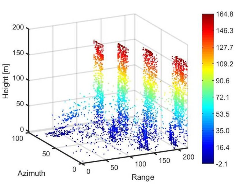
Remote Sens. 2020, 12, 3100                                                                         2 of 19

dedicated to developing new tomographic inversion algorithms and scatterers detectors in recent
decades [19–33]. In this manuscript, tomographic inversion algorithms refer to those aiming at
reconstructing “elevation profiles” from time series SAR images, whereas scatterers detectors refer to
those aiming at automatically detecting number of scatterers, their corresponding magnitude/strength
and precise elevation positions from the “elevation profiles”. Until now, the tomographic inversion
algorithms can be categorized into three groups, including back-propagation, spectrum estimation
and compressive sensing-based algorithms [5,19–30]. On the other hand, current scatterers detectors
can be categorized into three groups as well, such as Multi-Interferogram Complex Coherence
(MICC) based detectors, model order selectors, and Generalized Likelihood Ratio Test (GLRT) based
detectors [16,31–35].
      Notwithstanding, a large number of orbits are usually used for tomographic reconstruction,
in order to keep sufficient coherence. Previous study has shown that a single scatterer can always
be reliably detected when more than 5 orbits are used in tomographic reconstruction with X-band
spaceborne SAR data, whereas approximately more than 40 orbits are necessary for successful detection
of double scatterers [19]. However, X-band sensors have problems to handle both spatial coverage and
resolution. In many cases, there is no large number of acquisitions available. The minimum number of
tracks for tomographic inversion is only estimated for forest structure reconstruction, unfortunately
never for urban TomoSAR [36]. Different from the volume scattering mechanism in vegetated areas,
the signal inside one pixel of man-made structures is generally composed of components from several
scattering centers. Besides, there is no need to carry out tomographic reconstruction for every pixel
in urban areas. It is only necessary to carry out tomographic reconstruction for pixels with stable
back-scattering magnitude and high coherence (also referred to as persistent scatterers), instead of
all pixels. Since persistent scatterers are generally less affected by spatial and temporal decorrelation,
tomographic reconstruction of urban structures with limited number of images is therefore possible
and exploited in this article.
      Ideally speaking, the spatial baselines for tomographic SAR inversion should be uniformly
distributed. If the spatial span of baselines is determined for uniform baselines, the estimated elevation
resolution is determined [16]. The elevation resolution represents the minimal distinguishable distance
between two scatterers, which is the width of the elevation point response function (PRF) [16]. It can
be calculated with the following Equation:

                                                       λr
                                               ρs =                                                    (1)
                                                      2∆b
where ρs represents the elevation resolution, λ is the wavelength of SAR sensors, r is the target-sensor
distance in Line-Of-Sight (LOS) direction, and ∆b is the baseline aperture (the maximum difference
between orbits) of the SAR image stack [16]. The elevation resolution only depends on the baseline
aperture when the wavelength and height of sensors are determined. If we want to keep the elevation
resolution with limited number of SAR images, a possible solution should be increasing the spatial
interval between adjacent orbits and optimizing the baseline configuration in consideration of baseline
redundancy minimization.
     The optimal design of baselines in SAR has been studied for years, which can be categorized
into two different ways. One way is to set the interval between adjacent orbits as multiplies of
half-wavelength, such as minimum redundancy array (MRA), Restricted Minimum Redundancy
Array (RMRA) and Golomb Array (GA), etc. [37–39]. The other way is to design an optimal baseline
array with fixed number of elements and fixed baseline aperture based on bionics algorithms such
as artificial bee colony algorithm, memetic algorithm, and genetic algorithm, etc. [40–42]. In recent
years, baseline optimization has also been exploited for TomoSAR. Lu et al. has constructed a minimax
baseline optimization model based on non-uniform linear array for TomoSAR [43]. Bi et al. has
proposed a coherence of measurement matrix-based baseline optimization criterion and missing
data completion of unobserved baselines to facilitate wavelet-based Compressive Sensing TomoSAR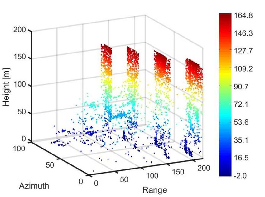
Remote Sens. 2020, 12, 3100 3 of 19
Remote Sens. 2020, 12, x FOR PEER REVIEW 3 of 19
(CS-TomoSAR) in forested areas [44]. Zhao et al. has explored the impact of baseline distribution
in spaceborne multistatic TomoSAR (SMS-TomoSAR) and proposed a baseline optimization method
optimization method under uniform-perturbation sampling with Gaussian distribution error [45].
under uniform-perturbation sampling with Gaussian distribution error [45]. However, most of
However, most of the above-mentioned research is conducted by simulations based on airborne
the above-mentioned research is conducted by simulations based on airborne system parameters.
system parameters. Unfortunately, very limited experimental result has been reported on the
Unfortunately, very limited experimental result has been reported on the optimization of spaceborne
optimization of spaceborne baselines for urban TomoSAR until now.
baselines for urban TomoSAR until now.
Targeting the above-mentioned problem, this paper focuses on finding an optimal baseline
Targeting the above-mentioned problem, this paper focuses on finding an optimal baseline
configuration of repeat-pass spaceborne SAR images for tomographic reconstruction using limited
configuration of repeat-pass spaceborne SAR images for tomographic reconstruction using limited
number of SAR images, which is called baseline optimization. In this paper, the minimum
number of SAR images, which is called baseline optimization. In this paper, the minimum redundancy
redundancy array (MRA) in wireless communication theory is innovatively applied for
array (MRA) in wireless communication theory is innovatively applied for tomographic baseline array
tomographic baseline array optimization, for the purpose of keeping equivalent elevation
optimization, for the purpose of keeping equivalent elevation resolution when only non-uniform
resolution when only non-uniform sampling and limited number of orbits are available.
sampling and limited number of orbits are available.
2. Methodology
2. Methodology
2.1. Tomographic
2.1. Phase Model
Tomographic Phase Model
In the
In the SAR
SAR image
image coordinate
coordinate system,
system, aa third
third coordinate
coordinate axis
axis orthogonal
orthogonal to to the
the azimuth–slant
azimuth–slant
range (x–r) plane is defined, called elevation (s) [6] as shown in Figure 1a. A focused
range (x–r) plane is defined, called elevation (s) [6] as shown in Figure 1a. A focused SAR image SAR imagecancan
be
be considered
considered as a as
2Daprojection
2D projection
of the of
3Dthe 3D back-scattering
back-scattering scenarioscenario
into the into the x–r
x–r plane [16].plane [16]. As
As shown in
shown in Figure 1b, the measurement of the resolution cell contains backscattered
Figure 1b, the measurement of the resolution cell contains backscattered signals from two different signals from two
different single-bounce
single-bounce scatterersscatterers
(scatterers(scatterers
A and B),A andthose
since B), since
twothose two single-bounce
single-bounce scatterers scatterers have
have the same
the same slant-range
slant-range distance to distance to the
the sensor andsensor
will and will be into
be focused focused into the
the same same resolution
resolution cell [21].cell [21].
With a
With a stack of N co-registered SAR acquisitions, we are able to reconstruct the
stack of N co-registered SAR acquisitions, we are able to reconstruct the backscattering profile along backscattering
profile
the alongdirection
elevation the elevation
for eachdirection
resolutionforcelleach resolution
with SAR cell with
tomography. The SAR tomography.
combination of thoseThe
N
combination of those N acquisitions forms
acquisitions forms the so-called elevation aperture.the so-called elevation aperture.
(a) 3D SAR coordinates (b) layovered double scatterers
1. 3D SAR
Figure 1. SAR coordinate
coordinatesystem
system(a)
(a)and
andtypical
typicallayover
layovereffect
effect
ofof double
double single-bounce
single-bounce scatterers
scatterers in
in urban
urban SAR SAR images
images (b).(b).
In a stack
stack of
of N
N co-registered
co-registered SAR
SAR acquisitions,
acquisitions, the complex value of a certain
certain resolution cell in
the nth image is considered as the integral of the real backscattering signals
nth image is considered as the integral of the real backscattering signals along elevation
along direction,
elevation
and represented
direction, by the following
and represented by the Equation
followingasEquation as
smax
Z smax
g n g=n = γ ( s )γ⋅(exp(
s)· exp ⋅ 2π ⋅ ξ n ·s⋅ s)·ds
− (j−j·2π·ξ ) ⋅ ds
n = n1,=2,1,· ·2,
· ,
N,N (2)(2)
− smax
−smax
where [−s−[ ]
s , s , s ] is the elevation span, ξ = −2bn /(λr) is the spatial frequency along elevation, γ(s)
where maxmaxmaxmax is the elevation nspan, ξ n =−2bn (λr) is the spatial frequency along
is the backscattering magnitude along the elevation direction [16]. There are N measurements in a
elevation, γ ( s ) is the backscattering magnitude along the elevation direction [16]. There are N
measurements in a tomographic data stack. The continuous reflectivity model could be
approximated by discretizing the function along s with a sampling frequency of L (L >> 0).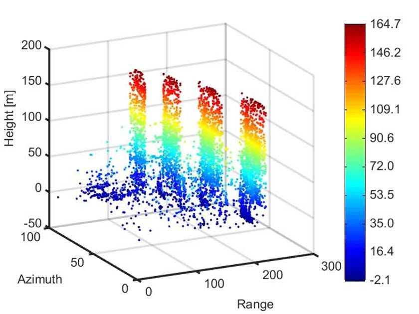
Remote Sens. 2020, 12, 3100                                                                       4 of 19

tomographic data stack. The continuous reflectivity model could be approximated by discretizing the
function along s with a sampling frequency of L (L >> 0).

                                             g = K ·γ + ε                                            (3)
                                         N×1    N×1 L×1   N×1

where g is the measurement vector with N elements gN , K is an N × L imaging operator, and γ is the
reflectivity vector along s with L elements [16]. ε is the noise term, which is assumed as independent
identically distributed complex zero mean and Gaussian. The noise could be neglected in the system
model if appropriate pre-processing of the data stack is conducted for real data analysis. Details about
the pre-processing are described in [5,12]. The objective of TomoSAR is to retrieve the backscattering
profile γ for each pixel from N measurements (gN ) and then use it to estimate scattering parameters,
such as the number of scatterers within a resolution cell, their elevations, as well as reflectivity,
with scatterers detectors [16,31–35].
     Among various tomographic reconstruction methods, Truncated Singular Value Decomposition
(TSVD) is commonly used in spaceborne TomoSAR due to its good performance and computational
simplicity [7]. On the other hand, Compressive Sensing (CS) based algorithms have been demonstrated
to have super-resolution power. However, its high computational complexity has prevented it from
being a useful tool for tomographic reconstruction of large areas on regular personal computers [22–24].
In our previous study, Two-step Iterative Shrinkage/Thresholding (TWIST) was proposed for TomoSAR
reconstruction as a balance between TSVD and CS [29,46]. The merits of TWIST in terms of
robustness, fast convergence speed, and super-resolution capability have been demonstrated by
both simulations and experiments on TerraSAR-X datasets [29]. Following tomographic reconstruction,
the number of scatterers, their corresponding strength/magnitude, and precise elevation positions are
automatically detected from the elevation profiles by scatterers detectors. Many scatterers detectors
have been proposed and assessed in literature. It is worth mentioning that with GLRT based detectors,
even simple inversion scheme like beamforming can achieve a very high detection rate on single and
double scatterers [19,31–35]. Since it is not our goal to compare different tomographic methods nor
scatterers detectors, tomographic reconstruction is conducted using both TWIST and classical TSVD,
combined with a common BIC-based detector in this article.
     Compared to the high resolution in azimuth and range direction, the relatively poor elevation
resolution does not necessarily mean that accuracy of estimated elevation is this poor. On the other
hand, the estimation accuracy of individual scatterers is defined by Cramer-Rao Lower Bound (CRLB),
which can be calculated with the following Equation.

                                                   λr
                                     σŝ =      √    √                                               (4)
                                             4π· NOA· 2SNR·σb

where NOA is the number of acquisitions, SNR is the signal to noise ratio, and σb is the standard
deviation of baselines [16].

2.2. Minimum Redundancy Array in SAR Tomography
     The Minimum Redundancy Array (MRA), also known as Minimum Redundancy Linear Array
(MRLA), was proposed in antenna array design in radio astronomy [37,47,48]. It is a subset of
non-uniform linear array which provides the largest aperture for a given number of elements or uses
the minimum number of elements to realize a given aperture [47–49]. It has been proved that the Mean
Square Error (MSE) and Cramer-Rao Bound (CRB) of MRAs are the least compared with coprime and
nested arrays [50,51]. A MRA is formed from a full antenna array by carefully eliminating redundant
antennas while the retained elements can generate all possible antenna separation between zero and
the maximum antenna length. Its merits come from the fact that it can provide the highest possible
resolution with minimized redundancy [51,52]. Numerically, redundancy R is defined as the number
of pairs of antennas divided by maximum spacing of the linear array. As shown in literatures [37,47],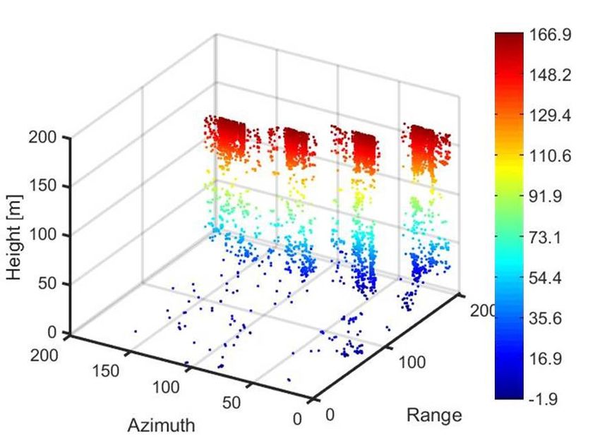
Remote
 RemoteSens.  2020,12,
        Sens.2020,  12,3100
                        x FOR PEER REVIEW                                                                                        55of
                                                                                                                                    of19
                                                                                                                                       19

 number of elements, R = 2( N − 1) / ( N + 2) for a MRA with even number of elements, where N
R = 2N (N − 1)/(N + 1)2 for a MRA with odd number of elements, R = 2(N − 1)/(N + 2) for a MRA
 is theeven
with     number
              numberof elements     in a linear
                          of elements,   wherearray.
                                                 N is the number of elements in a linear array.
       According       to  literatures  [37,47],
      According to literatures [37,47], when the when    thenumber
                                                             numberof  ofelements
                                                                          elementsisisless
                                                                                         lessthan
                                                                                              than5,5,zero-redundancy
                                                                                                        zero-redundancy
 arrays   exist.  In  other   words,   there  are only  four  zero-redundancy      arrays,
arrays exist. In other words, there are only four zero-redundancy arrays, which have been   which    have   beenelegantly
                                                                                                                   elegantly
 proved     in literature    [52]. The  four  zero-redundancy      arrays and   their spatial   distributions
proved in literature [52]. The four zero-redundancy arrays and their spatial distributions are shown             are  shown
 inFigure
in   Figure2.2. Except
                  Except forfor the
                                 the zero
                                     zero spacing
                                           spacing (spatial
                                                     (spatial distance)
                                                              distance) in
                                                                         in the
                                                                            the trivial
                                                                                 trivial case
                                                                                          case of
                                                                                                of single-element
                                                                                                   single-element array,array,
 each   spacing    is  presented    only  once.  For  example,   spacing  between    adjacent   elements
each spacing is presented only once. For example, spacing between adjacent elements are 1, 3, and            are  1, 3, and2,2,
 respectively,for
respectively,      forthethe  4-element
                           4-element       array,
                                       array,      leading
                                              leading       to a maximum
                                                       to a maximum     spatialspatial distance
                                                                                distance   of 6. Inof  6. Inwords,
                                                                                                    other     other there
                                                                                                                      words,is
 there   is  one,   and    only   one,  pair  of  elements   separated   by   each   multiple    of
one, and only one, pair of elements separated by each multiple of the unit spacing in zero-redundancythe  unit   spacing    in
 zero-redundancy          arrays,  resulting  in a  maximum     spacing  equal   to the distance
arrays, resulting in a maximum spacing equal to the distance between the left-end and right-end     between    the   left-end
 and right-end
elements.           elements.
              As shown            As shown
                             by Figure   2, theby  Figure 2,and
                                                3-element    the4-element
                                                                  3-elementarrays
                                                                              and 4-element
                                                                                     are the onlyarrays
                                                                                                     twoare   the only two
                                                                                                           non-uniformly
 non-uniformly        distributed    arrays
distributed arrays with zero-redundancy.     with   zero-redundancy.

      Figure 2. The four zero-redundancy linear arrays and their spatial distribution, where red diamonds
       Figure 2. The four zero-redundancy linear arrays and their spatial distribution, where red diamonds
      represent spatial positions of elements, white bars represent spacing (spatial distance) between
       represent spatial positions of elements, white bars represent spacing (spatial distance) between
      adjacent elements.
       adjacent elements.
      For linear arrays with more than 4 elements, redundancy is always larger than 0, and there has to be
some For   linear arrays
       configuration      with
                      of the    more than
                             elements  which 4 elements,  redundancy
                                               leads to minimum          is alwaysHowever,
                                                                    redundancy.    larger than
                                                                                             it is0,
                                                                                                  notand  there
                                                                                                       easy        has
                                                                                                             to find
 to be  some   configuration   of the elements   which   leads to  minimum     redundancy.    However,
the optimum MRA configurations for a large number of elements. Wherein, the relationship between            it  is not
 easy
the     to find
     number   of the
                 MRAoptimum
                       elementsMRA M andconfigurations     for N
                                           the array aperture  a large
                                                                   can benumber
                                                                           given byoftheelements.
                                                                                         followingWherein,
                                                                                                      theorem: the
 relationship
      For any M > 3, a set of positive integers {x1 , x2 , . . . , xM } can always be selected togiven
                between   the number    of MRA    elements  M  and   the array  aperture  N  can  be    satisfybythe
                                                                                                                   the
 following   theorem:
condition 0 = x < x2 < . . . < x = N, and for any integer i(0 ≤ i ≤ N ), there are always two elements
                                         M
                     1
with aFor   any M of
         difference  > 3,  a {x
                        i in               . . . , xM }, and
                             set1 , xof2 , positive            M2 /N
                                                         integers    {x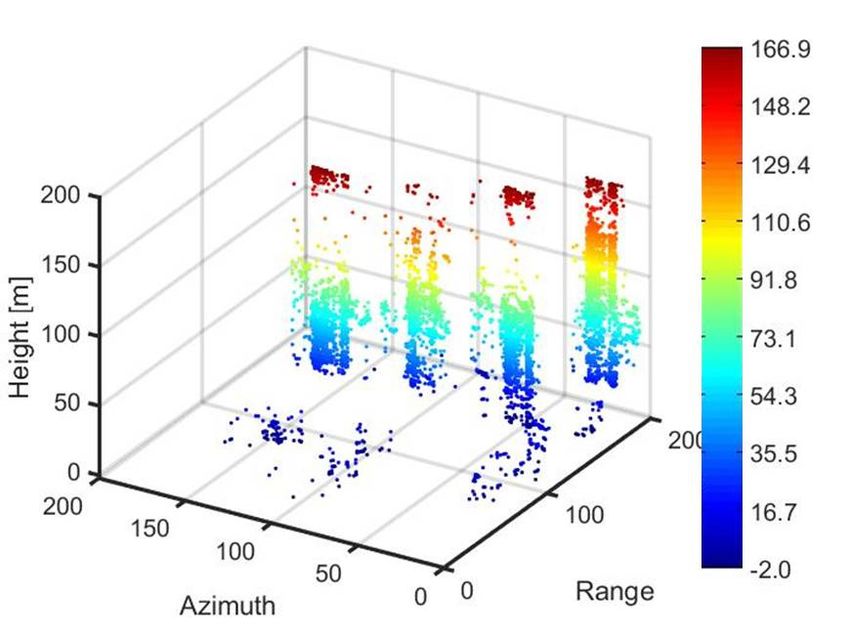
Remote Sens. 2020, 12, 3100                                                                                           6 of 19

until the redundancy reaches minimum. Therefore, the baseline distribution of MRA orbits is not
strictly non-uniform, but uniform with missing orbits.
      When trying to find the MRA orbits for TomoSAR, the spatial positions of SAR sensor at each revisit
is considered as elements of the array, and the neighboring baselines are considered as spacing between
elements. In order to keep equivalent elevation resolution, the orbits with maximum perpendicular
baselines (∆b = b1 − bN ) are first selected, and the smallest distance between the end-orbit and its
neighbor orbit is chosen as spacing unit (u). So the initial three elements in a baseline array is configured
as {.u. (∆b − u).}, where dots represent positions of the orbit and numbers refer to the spacing. Then,
between spacing (∆b − u), a fourth orbit can be found located at two spacing units with reference two the
end-orbits. So the baseline array becomes {.u.2u.(∆b − 3u).} or {.u.(∆b − 3u).2u.}. Following this scheme,
the MRA orbits can be found iteratively. In fact, the baselines are not exactly uniformly distributed,
we can only find MRA-like orbits close to the ideal MRA positions by selecting the combination with
minimum standard deviation with reference to ideal MRA positions.
      Let us assume the original baseline array with N elements is (b1 , b2 , . . . , bN )T , and the spacing
unit is selected as u = b1 − b2 . So, the number of normalized baselines should be X = ∆b/u. For a
given X, the normalized distributions of MRA elements have already been given in Table 1. Table 1
depicts the designed MRA orbits for 7 ≤ M ≤ 10 and their equivalent number of uniform orbits with
reference to an interval of u. If the number of MRA orbits is 10, the corresponding number of uniform
orbits is 37, with 36 uniform baselines. Considering the interval of x in uniform baselines, the baseline
aperture should be 36u. The positions of MRA orbits should be {0,1,3,6,13,20,27,31,35,36} multiplied by
u, respectively. As shown in Table 1, the arrangement of elements for MRA is not unique. There are
three different MRA orbit arrangements for M = 9, two different arrangements for M = 8, and five
different MRA orbit arrangements for M = 7. These different arrangements have been studied and
evaluated in [53,54]. Since it is not our goal to compare different MRA orbits, only one set of MRA orbits
(highlighted in bold font in Table 1) for each M is selected for tomographic simulations in this paper.

                   Table 1. Normalized distributions of minimum redundancy array (MRA) orbits.

              M       N       Normalized Positions of MRA Orbits with Reference to an Interval of u
              10      37                                    0,1,3,6,13,20,27,31,35,36
               9      30                                     0,1,2,14,18,21,24,27,29
               9      30                                     0,1,3,6, 13,20,24,28,29
               9      30                                     0,1,4,10,16,22,24,27,29
               8      24                                       0,1,2,11,15,18,21,23
               8      24                                       0,1,4,10,16,18,21,23
               7      18                                           0,1,2,3,8,13,17
               7      18                                          0,1,2,6,10,14,17
               7      18                                          0,1,2,8,12,14,17
               7      18                                          0,1,2,8,12,15,17
               7      18                                         0,1,8,11,13,15,17
      M represents number of MRA orbits; N represents number of uniform orbits; N − 1 represents the number of
      uniform baselines.

    Let us assume the optimal virtual positions of MRA baselines with M elements are (b1 , b2 , . . . , bM )T ,
and M < N. By an exhaustive search, the real orbits close to (b1 , b2 , . . . , bM )T are (b1 , b02 , . . . , b0M−1 , bM )T .
Actually, there could be many choices for (b1 , b02 , . . . , b0M−1 , bM )T . The best fit of MRA-like orbits can be
found by calculating the minimum Root Mean Square Error (RMSE) between (b1 , b02 , . . . , b0M−1 , bM )T
and (b1 , b2 , . . . , bM )T . Then the expressions in Equations (2) and (3) can be optimized as
                                      Z    smax
                               gm =               γ(s)· exp(− j·2π·ξm ·s)·ds m = 1, 2, · · · , M                         (5)
                                          −smax

                                                        ξm = −2bm /(λr)                                                  (6)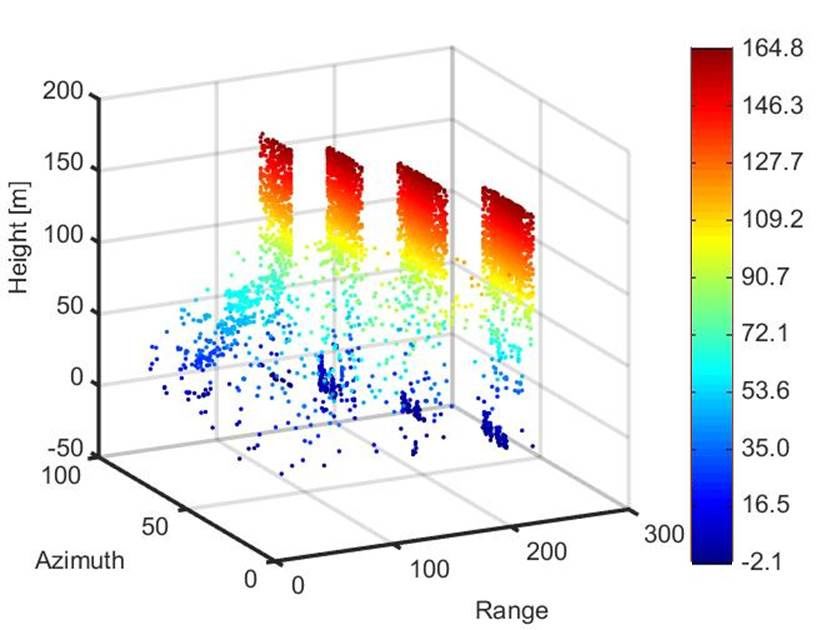
can be optimized as
s max
gm = − smax
γ ( s ) ⋅ exp( − j ⋅ 2π ⋅ ξ m ⋅ s ) ⋅ ds m = 1, 2, , M (5)
Remote Sens. 2020, 12, 3100
ξm = −2bm (λr) (6)19
7 of
g = K⋅γ + ε (7)
M ×L M ×1
g = K · γL×+
M ×1 1
ε (7)
M×1 M×L L×1 M×1
3. Tomographic Simulations
3. Tomographic Simulations
We designed four groups of uniform orbits with perpendicular baseline aperture of 1000 m in
We designed four groups of uniform orbits with perpendicular baseline aperture of 1000 m in
the simulation. The numbers of uniform orbits are 37, 30, 24, and 18, respectively. The baseline
the simulation. The numbers of uniform orbits are 37, 30, 24, and 18, respectively. The baseline
distributions of the four groups are shown in Figure 3, where the blue dots represent uniform orbits.
distributions of the four groups are shown in Figure 3, where the blue dots represent uniform orbits.
Their corresponding MRA orbits are also selected following Table 1, as marked with red triangles in
Their corresponding MRA orbits are also selected following Table 1, as marked with red triangles in
Figure 3. Compared to the uniform orbits, the numbers of MRA orbits are dramatically reduced.
Figure 3. Compared to the uniform orbits, the numbers of MRA orbits are dramatically reduced.
(a) (b)
(c) (d)
Figure3.3.The
Figure Thesimulated
simulated uniform
uniform orbits
orbits and
and their corresponding MRA
their corresponding MRA orbits:
orbits: (a)
(a)1010MRA
MRAout outofof37
37uniform
uniformorbits;
orbits;(b)
(b)99MRA
MRAout
outof
of 30
30 uniform
uniform orbits;
orbits; (c)
(c) 8 MRA out of 24 uniform orbits; (d) 7MRA
8 MRA out of 24 uniform orbits; (d) 7 MRA
out of 18 uniform orbits.
out of 18 uniform orbits.
Generally,
Generally,single-scatterer
single-scattererand anddouble-scatterers
double-scattererspixels
pixelsmost
mostcommonly
commonlyoccuroccurininlayover
layoverareas
areas
ofofhigh-resolution
high-resolution SAR images for urban scenarios, these two cases are usually consideredfor
SAR images for urban scenarios, these two cases are usually considered for
TomoSAR [11]. The occurrence of more than two scatterers can increase in medium
TomoSAR [11]. The occurrence of more than two scatterers can increase in medium resolution SAR resolution SAR
images
imageslike Sentinel-1,
like Sentinel-1,butbut
it also depends
it also dependson theon
geometry of the ground
the geometry of the scene
ground andscene
on theandelevation
on the
resolution [11]. The merit of TomoSAR is its capability in separating multiple scatterers
elevation resolution [11]. The merit of TomoSAR is its capability in separating multiple scatterers (at least two) (at
superimposed inside one resolution cell. Therefore, simulations on double scatterers
least two) superimposed inside one resolution cell. Therefore, simulations on double scatterers are are conducted
inconducted
this section. Two
in this scatterers
section. Two located
scatterers −20 m at
atlocated and
−2020mmandwith
20 mnormalized reflectivity
with normalized of 1 and
reflectivity of 1
0.6 respectively are simulated. The X-band system parameters and the four groups
and 0.6 respectively are simulated. The X-band system parameters and the four groups of orbits of orbits designed
indesigned
Figure 3 arein initialized
Figure 3 arefor simulation.
initialized forThesimulation.
reconstructed elevation
The profiles elevation
reconstructed from uniform orbitsfrom
profiles in
noise free case are shown in Figure 4a–d. When the orbits remain uniformly distributed
uniform orbits in noise free case are shown in Figure 4a–d. When the orbits remain uniformly with identical
baseline aperture, tomographic performances of both methods are not corrupted by simply reducing
the number of orbits from 37 to 18.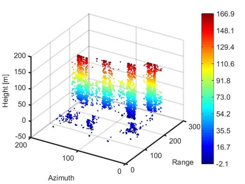
Remote Sens. 2020, 12, x FOR PEER REVIEW                                                                   8 of 19

 distributed with identical baseline aperture, tomographic performances of both methods are not
Remote Sens. 2020, 12, 3100                                                              8 of 19
 corrupted by simply reducing the number of orbits from 37 to 18.

                   (a) 37 Uniform Orbits                                    (e) 10 MRA Orbits

                   (b) 30 Uniform Orbits                                     (f) 9 MRA Orbits

                    (c) 24 Uniform Orbits                                    (g) 8 MRA Orbits

                   (d) 18 Uniform Orbits                                     (h) 7 MRA Orbits

        Figure4. 4.Tomographic
      Figure        Tomographicperformance
                                  performanceofofTWIST
                                                    TWISTand
                                                          andTSVD
                                                              TSVDonondouble
                                                                       doublescatters
                                                                               scattersusing
                                                                                        usinguniform
                                                                                              uniformorbits
                                                                                                       orbits
      (a–d) and
        (a–d) and MRA
                    MRAorbits (e–h)
                         orbits     inin
                                (e–h)  noise free
                                         noise    case.
                                               free case.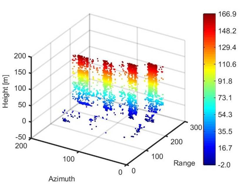
Remote Sens. 2020, 12, x FOR PEER REVIEW 9 of 19
Remote Sens. 2020, 12, 3100 9 of 19
If the uniform orbits are replaced by their corresponding MRA orbits, TSVD suffers from
dramatic increase orbits
If the uniform of sidelobes, withby
are replaced normalized reflectivity
their corresponding of approximately
MRA 0.6 for
orbits, TSVD suffers thedramatic
from largest
sidelobe,
increase ofas shown in
sidelobes, Figure
with 4e–h. The
normalized strong sidelobes
reflectivity in TSVD profiles
of approximately may
0.6 for the lead sidelobe,
largest to false detection
as shown
of a third scatterer. On the other hand, TWIST shows a much better resistance against
in Figure 4e–h. The strong sidelobes in TSVD profiles may lead to false detection of a third scatterer. sidelobes,
with
On thethe largest
other hand,sidelobe
TWISTsmaller
shows athan
much 0.23, see resistance
better Figure 4h.against
By comparing
sidelobes,thewith
fourthe
figures
largestinsidelobe
Figure
4e–h, we
smaller can0.23,
than tell that
see the normalized
Figure strengths ofthe
4h. By comparing sidelobes in neither
four figures TSVD4e–h,
in Figure nor TWIST
we canprofiles
tell thatare
the
further increased when the number of MRA orbits drops from 10 to 7. This means
normalized strengths of sidelobes in neither TSVD nor TWIST profiles are further increased when the that reducing the
numberofofMRA
number MRAorbits
orbitsdrops
would also
from 10not
to 7.result in a dramatic
This means increase
that reducing theofnumber
sidelobes, as long
of MRA as MRA
orbits would
orbits are used.
also not result in a dramatic increase of sidelobes, as long as MRA orbits are used.
Inthe
In thesecond
second simulation,
simulation, white
white Gaussian
Gaussian noisenoise at different
at different SNR islevels
SNR levels addedistoadded to the
the simulated
simulated signal. The reconstructed profiles of double scatterers from 10 MRA
signal. The reconstructed profiles of double scatterers from 10 MRA orbits at different SNR levels orbits at different
SNR levels are depicted in Figure 5. As the SNR decreases, the sidelobes go up gradually for both
are depicted in Figure 5. As the SNR decreases, the sidelobes go up gradually for both methods,
methods, however the sidelobes in TWIST profiles are much smaller than in TSVD profiles. By
however the sidelobes in TWIST profiles are much smaller than in TSVD profiles. By comparing
comparing Figure 5 with Figure 4a, a preliminary conclusion that tomographic reconstruction can be
Figure 5 with Figure 4a, a preliminary conclusion that tomographic reconstruction can be corrupted if
corrupted if the SNR levels are reduced from infinite (noise free) to 1, since strong sidelobes may
the SNR levels are reduced from infinite (noise free) to 1, since strong sidelobes may bury the weak
bury the weak scatterer’s signal or be mistaken as another scatterer, as shown in Figure 5c,d.
scatterer’s signal or be mistaken as another scatterer, as shown in Figure 5c,d. Nevertheless, TWIST
Nevertheless, TWIST presents better resistance against noise compared with TSVD.
presents better resistance against noise compared with TSVD.
(a) SNR = 10 (b) SNR = 5
(c) SNR = 2 (d) SNR = 1
Figure5.5.Tomographic
Figure Tomographic performance
performance of TWIST and TSVD
TWIST and TSVD on
on double
doublescatters
scattersatatdifferent
differentSNR
SNRlevels
levels
when
when1010MRA
MRAorbits
orbitsare
areused.
used.
The
TheCRLBs
CRLBsfor forMRA
MRA 10 10
orbits andand
orbits 37 uniform orbits
37 uniform at different
orbits SNR levels
at different SNR are depicted
levels in Figure
are depicted in6.
Although there is a slight drop on the CRLB using MRA orbits instead of uniform orbits,
Figure 6. Although there is a slight drop on the CRLB using MRA orbits instead of uniform orbits, fortunately
the largest decrease
fortunately the largestis within
decrease0.3ismwithin
when0.3SNRm is 1 dB.SNR
when Thisisdifference
1 dB. Thisnarrows
differencequickly
narrowsas the SNR
quickly
increases.
as the SNRFor SNR >=
increases. 5 dB,
For SNRthe>= difference is smalleristhan
5 dB, the difference 0.1 than
smaller m. The slight
0.1 m. Thedifferences on CRLBs
slight differences on
indicate that using MRA orbits instead of uniform orbits does not corrupt the estimation
CRLBs indicate that using MRA orbits instead of uniform orbits does not corrupt the estimation accuracy
very much.
accuracy very much.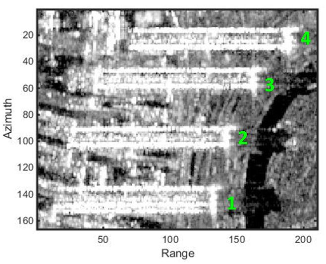
Remote Sens. 2020, 12, 3100 10 of 19
Remote Sens. 2020, 12, x FOR PEER REVIEW 10 of 19
Figure Cramer-Rao
6. 6.
Figure Lower
Cramer-Rao Bound
Lower (CRLB)
Bound at at
(CRLB) different SNR
different levels.
SNR levels.
AnAn important
important characteristic
characteristic forforevaluating
evaluating thethe
tomographic
tomographic performance
performance ofofMRAMRA orbits
orbits is is
to to
analyze the successful detection rate of scatterers at different SNR levels.
analyze the successful detection rate of scatterers at different SNR levels. In order to do this, a Monte In order to do this, a Monte
Carlo
Carlo simulation
simulation onon 1000
1000 double
double scatters
scatters is conducted.
is conducted. For
For thethe
purpose
purpose ofofavoiding
avoiding influence
influence caused
caused
bybydistance or amplitude ratios (γ2/γ1) between the two scatterers,
distance or amplitude ratios (γ2/γ1) between the two scatterers, identical scatterers are used identical scatterers are used forfor
thethe
1000
1000 double-scatterers pixels. A strong scatterer with normalized reflectivity of 1 is located atat
double-scatterers pixels. A strong scatterer with normalized reflectivity of 1 is located −40
−40m,m,andand a weak
a weak scatterer
scatterer withwith normalized
normalized reflectivity
reflectivity of 0.8of 0.8 is located
is located at 40 m.atAt 40each
m. SNRAt each
levelSNR (1–15
level
dB),(1–15
random dB), white
random white Gaussian
Gaussian noise is added noise is to added
the 1000 to simulated
the 1000 simulated
pixels. The pixels. The normalized
normalized reflectivity
reflectivity
and elevation and elevation
positionposition are automatically
are automatically detecteddetected
usingusing modelmodel selection
selection algorithm
algorithm basedon
based
onBayesian
BayesianInformation
InformationCriterion Criterion (BIC)(BIC) [32].
[32]. The
The successful
successful detection
detectionrates ratesare arecalculated
calculatedforfor eacheach
scatterer at various SNR levels. A successful detection is defined
scatterer at various SNR levels. A successful detection is defined when the estimated elevation when the estimated elevation is is
within
within a theoretical
a theoretical resolution cell centered
resolution by the real
cell centered by elevation position, meaning
the real elevation position,that the maximum
meaning that the
difference between the estimated and the real elevation is smaller
maximum difference between the estimated and the real elevation is smaller than half of the than half of the elevation resolution
in elevation
our simulations.
resolution in our simulations.
The The detection
detection rates of double
rates of double scatterers at different
scatterers SNR levels
at different SNR are levelsshown are in Figurein7.Figure
shown As shown 7. As
byshown
the dashedby the dashed lines in Figure 7a, successful detection rates of both scatterers at variousare
lines in Figure 7a, successful detection rates of both scatterers at various SNR levels SNR
close to 1are
levels usingcloseuniform
to 1 using orbits, no matter
uniform what
orbits, nomethod
matter what(TWIST or TSVD)
method (TWISTis used. WhenisMRA
or TSVD) used.orbits
When
areMRA
usedorbits
instead, aredetection
used instead,rates of scattererrates
detection 1 drop ofslightly
scatterer for1 both
dropmethods,
slightly for with the methods,
both lowest detection
with the
rate of approximately 0.7 when SNR is 1, as shown by the solid blue
lowest detection rate of approximately 0.7 when SNR is 1, as shown by the solid blue and red lines and red lines in Figure 7a. On the in
other hand,
Figure 7a.detection
On the other rates hand,
of scatterer
detection2 drop dramatically
rates of scatterer when MRA
2 drop orbits are used,
dramatically when especially
MRA orbits whenare
TSVD method is used for tomographic reconstruction at low
used, especially when TSVD method is used for tomographic reconstruction at low SNR levels,SNR levels, as shown by the green and as
black solid lines in Figure 7a. At identical SNR levels, the detection rates
shown by the green and black solid lines in Figure 7a. At identical SNR levels, the detection rates of of scatterer 2 is generally lower
than scatterer
scatterer 2 is1 using
generallyMRAlower orbits, thisscatterer
than is probably caused
1 using MRAby the reduced
orbits, this sampling
is probably along elevation
caused by the
aperture. Nevertheless, since it is useless to do tomographic analysis
reduced sampling along elevation aperture. Nevertheless, since it is useless to do tomographic if there is no strong backscattering
signal in a pixel
analysis if there(e.g.,isdark points on
no strong flat surface), tomographic
backscattering signal in a pixel analysis
(e.g.,is usually
dark pointsconductedon flatonsurface),
pixels
with strong backscattering
tomographic analysis issignal usually (soconducted
called bright onpoints
pixelsinwithamplitude
strongimages). Previous
backscattering study(so
signal shows
called
that SNRs of these bright points (pixels with strong backscattering
bright points in amplitude images). Previous study shows that SNRs of these bright points (pixels signal) are generally larger than
10with
dB [9]. At SNR
strong level of 10 dB,
backscattering the detection
signal) rates oflarger
are generally both scatterers
than 10 dB from [9].MRA
At SNRorbitslevel
would of be
10 larger
dB, the
than 0.95 if TWIST method is used. Therefore, the decrease of successful
detection rates of both scatterers from MRA orbits would be larger than 0.95 if TWIST method is detection rates using MRA
orbits
used. at Therefore,
low SNR levels is to some
the decrease of extent
successfulneglectable
detection forrates
TWIST method,
using MRAcomparedorbits at low to the
SNRadvantages
levels is to
in some
dramatically reduced number
extent neglectable for TWISTof images.method, compared to the advantages in dramatically reduced
number of images.Remote Sens. 2020, 12, 3100 11 of 19
Remote Sens. 2020, 12, x FOR PEER REVIEW 11 of 19
(a) SC1 = −20 m, γ1 = 1; SC2 = 20, γ2 = 0.8; (b) SNR = 10; SC1 = −40 m, γ1 = 1; SC2 = 40 m;
SNR Changes γ2/γ1 changes
7. Successful detection rate of 1000 simulated double-scatterer pixels at different SNR levels
Figure 7. levels
(a) and
(a) and normalized
normalized amplitude ratios (γ2/γ1) (b), where SC abbreviates from scatterer and γ is the
normalized reflectivity
reflectivity (amplitude).
(amplitude).
In
In order
order to to analyze
analyze the the successful
successful detection
detection ratesrates ofof the
the weak
weak scatterer
scatterer when
when the the amplitude
amplitude ratio ratio
between
between two two scatterers
scatterers (γ2/γ1)
(γ2/γ1) changes,
changes, aa second second MonteMonte CarloCarlo simulation
simulation isis carried
carried out. out. InIn this
this
simulation, a strong scatterer with normalized amplitude of 1 located
simulation, a strong scatterer with normalized amplitude of 1 located at −40 m and a weak scatterer at −40 m and a weak scatterer
located
locatedatat4040mm with
withnormalized
normalized amplitude
amplitude changes from 0.1
changes from to 10.1
aretosimulated. Random Random
1 are simulated. white Gaussianwhite
noise
Gaussian withnoise
SNR withof 10SNR dB isofadded
10 dBto is 1000
added simulated pixels for pixels
to 1000 simulated each amplitude ratio. Both
for each amplitude uniform
ratio. Both
orbits
uniform orbits and MRA orbits are used for tomography. As shown by the red and blue lines7b,
and MRA orbits are used for tomography. As shown by the red and blue lines in Figure in
detection
Figure 7b,rates of scatterer
detection rates 1ofisscatterer
always about 1 no matter
1 is always aboutwhat 1 nomethod
matter and whatwhatmethod kind andof orbits
whatare used.
kind of
On theare
orbits other hand,
used. Ondetection
the otherrate of scatterer
hand, detection 2 increases when γ2/γ1
rate of scatterer increaseswhen
2 increases towards γ2/γ1 1, as shown
increases
by the green
towards 1, asandshown black by lines in Figure
the green 7b. The
and black low
lines in detection
Figure 7b.rate Theoflow scatterer
detection 2 israte
probably due to2
of scatterer
interference
is probably due of sidelobes of scatterer
to interference 1. If theof
of sidelobes amplitude
scatterer ratio is 0.4,
1. If the detection
amplitude rates
ratio is of
0.4,scatterer
detection 2 using
rates
both methods from uniform orbits approximate to 1. On the other
of scatterer 2 using both methods from uniform orbits approximate to 1. On the other hand, TWIST hand, TWIST has a detection rate of
0.82 on scatterer 2 from MRA orbits when amplitude ratio is 0.4,
has a detection rate of 0.82 on scatterer 2 from MRA orbits when amplitude ratio is 0.4, whereas whereas TSVD only reaches detection
rate
TSVD of 0.5
onlyonreaches
scattererdetection
2. As the rateamplitude
of 0.5 ratio increases2.toAs
on scatterer 0.6,the
detection
amplituderate of TWIST
ratio on scatterer
increases to 0.6,2
reaches 1 from MRA orbits. However, detection rate of TSVD
detection rate of TWIST on scatterer 2 reaches 1 from MRA orbits. However, detection rate of TSVDon scatterer 2 can only reach 1 when
amplitude
on scattererratio 2 can is only
higher than10.8
reach whenfrom MRA orbits.
amplitude ratioTherefore,
is higher than using0.8 MRAfrom orbits
MRAinstead
orbits.of uniform
Therefore,
orbits
using doesMRAnot affect
orbits the detection
instead of uniform rateorbits
of thedoesweaknot scatterer
affect theas long as therate
detection amplitude
of the weakratio is higher
scatterer
than 0.6 and TWIST is used for tomographic reconstruction. Unfortunately,
as long as the amplitude ratio is higher than 0.6 and TWIST is used for tomographic reconstruction. TSVD is not able to remain
equivalent
Unfortunately, detection
TSVD rateis from
not MRAable to orbits,
remainwithequivalent
amplitude ratios smaller
detection ratethan
from 0.8.MRA orbits, with
Besides SNR values
amplitude ratios smaller than 0.8. and amplitude ratios, distance between double scatterers also has an impact
on detection
Besides SNR rates values
of both and scatterers.
amplitude A thirdratios,Monte Carlobetween
distance simulation is conducted
double scatterers toalso assess
has the
an
detection
impact onrates of double
detection rates scatterers when distance
of both scatterers. A thirdbetween
Monte Carlo scatterers change.is In
simulation this Monte
conducted Carlo
to assess
simulation,
the detection scatterer
rates of1 double
with normalized
scatterers amplitude
when distance of 1 isbetween at −20 m. change.
located scatterers The distanceIn this between
Monte
two
Carlo scatterers
simulation, varies from 0 1towith
scatterer 2.5 times of the elevation
normalized amplitude resolution. Random
of 1 is located at white
−20 m. Gaussian noise
The distance
with
betweenSNR two of 10scatterers
dB is added to 1000
varies fromsimulated
0 to 2.5 pixels
times for of
each thedistancing.
elevation Figure 8 shows
resolution. the detection
Random white
rates whennoise
Gaussian distance
withbetween
SNR of double
10 dB is scatterers
added to changes. As shownpixels
1000 simulated in Figure 8a, when
for each the normalized
distancing. Figure 8
amplitude of scatterer
shows the detection 2 iswhen
rates 0.8, detection rates of scatterer
distance between 1 is generally
double scatterers changes.closeAstoshown
1 regardless
in Figure of the
8a,
distance, except for a slight drop at distances close to the theoretical
when the normalized amplitude of scatterer 2 is 0.8, detection rates of scatterer 1 is generally close elevation resolution. This slight
drop is caused by
to 1 regardless of interference
the distance,ofexcept scattererfor a2 slight
on scatterer
drop at 1. distances
The interference
close toeffect gets stronger
the theoretical when
elevation
amplitude
resolution. of scatterer
This slight 2dropincreases
is causedto 1, by
as shown by theofsudden
interference scattererfluctuation
2 on scattereron the1.detection rates of
The interference
scatterer
effect gets 1 instronger
Figure 8b. whenNevertheless,
amplitudethe ofinterference
scatterer 2 effect of uniform
increases to 1, orbits
as shown is even bystronger
the suddenthan
MRA orbits,on
fluctuation bythe
comparing
detection the depth
rates of of valleys1ininprofiles
scatterer Figure of 8b.scatterer 1, as shown
Nevertheless, by the red and
the interference blue
effect of
lines
uniformin Figure
orbits8b. This is
is even simplythan
stronger because MRA MRAsorbits,arebyinitially
comparingdesigned for interference
the depth of valleyscancelation
in profiles in of
radio astronomy.
scatterer 1, as shown by the red and blue lines in Figure 8b. This is simply because MRAs are
initially designed for interference cancelation in radio astronomy.Remote Sens.
Remote 2020,
Sens. 12,12,
2020, 3100
x FOR PEER REVIEW 1219
12 of of 19
(a) SC1 = −20 m, γ1 = 1; Distance between SC1 and SC2 (b) SC1 = −20 m, γ1 = 1; Distance between SC1 and SC2
changes, γ2 = 0.8; SNR = 10 changes, γ2 = 1; SNR = 10
Figure
Figure 8. Successful
8. Successful detection
detection rates
rates of double
of double scatterers
scatterers whenwhen distance
distance betweenbetween both scatterers
both scatterers changes,
changes, where SC abbreviates from scatterer, γ is the normalized reflectivity
where SC abbreviates from scatterer, γ is the normalized reflectivity (amplitude). (amplitude).
This
This interferenceeffect
interference effectbetween
between two two scatterers
scatterers has has already
alreadybeen beendiscussed
discussedinin literature
literature[9][9]
andand
presentedininour
presented oursimulations
simulations as as well.
well. IfIftwo twoscatterers
scatterers areare
close enough,
close enough,the the
estimated
estimatedlocations of
locations
of scatterers
scatterersmay maybe beshifted
shiftedby bythe
thesidelobes
sidelobesofofnearby nearbyscatterers,
scatterers,leading
leading totodecrease
decrease of of
successful
successful
detection
detection rates,
rates, eveneven
withwith
twotwo scatterers
scatterers further further
apartapart thanelevation
than the the elevation
resolutionresolution
[16]. The [16]. The
elevation
elevation estimate of one scatterer is systematically biased by the sidelobes
estimate of one scatterer is systematically biased by the sidelobes of other scatterers and vice versa, of other scatterers and
vicethough
even versa, the
even though
SNR the[16].
is high SNRAs is high
shown [16].
by As shown
Figure by interference
8, the Figure 8, theofinterference
the strong of the strong
scatterer on the
scatterer on the weak one is much more serious than the weak one on
weak one is much more serious than the weak one on the strong one. On one hand, the weak scatterer the strong one. On one hand,
the weak scatterer only causes a slight detection rate fluctuation on the strong one when their
only causes a slight detection rate fluctuation on the strong one when their distance increases from
distance increases from 0 to 1.5 times of the resolution. In Figure 8a, scatterer 1 is assumed to be
0 to 1.5 times of the resolution. In Figure 8a, scatterer 1 is assumed to be stronger than scatterer 2,
stronger than scatterer 2, with normalized amplitude of 1 and 0.8, respectively. The detection rate of
with normalized amplitude of 1 and 0.8, respectively. The detection rate of scatterer 1 only shows a
scatterer 1 only shows a slight drop when then distance between two scatterers is smaller than 1.5
slight drop when then distance between two scatterers is smaller than 1.5 times of the resolution. If the
times of the resolution. If the normalized amplitude of scatterer 2 is comparable with scatterer 1, its
normalized amplitude of scatterer 2 is comparable with scatterer 1, its interference on scatterer 1 gets
interference on scatterer 1 gets stronger, leading to deeper fluctuation of detection rate on scatterer
stronger, leading to deeper
1, as shown in Figure 8b. fluctuation
Therefore, the of detection
case of two rate on scatterer
comparable 1, as shown
scatterers is theinworst
Figurecase,
8b. Therefore,
instead
theofcase of two comparable scatterers is the worst case, instead of the optimal
the optimal one. If scatterer 2 gets even stronger, it will become the strong one and scatterer one. If scatterer 2 gets
1
even
willstronger,
become the it will
weakbecome
one. On thethe
strong
otherone hand, and thescatterer 1 will become
strong scatterer the weak
will definitely buryone.theOn theone
weak other
hand, the distance
if their strong scatterer
is smallerwill definitely
than bury the
the elevation weak oneAsif shown
resolution. their distance
by Figureis smaller
8a,b, thethan the elevation
detection rate
resolution. As shown by Figure 8a,b, the detection rate of scatterer 2 is 0 when
of scatterer 2 is 0 when distance between two scatterers is smaller than the elevation resolution. The distance between two
scatterers
detection is rate
smaller than the2elevation
of scatterer increasesresolution.
gradually from The detection
0 to 1 with ratedistance
of scatterer 2 increases
between gradually
two scatterers
from 0 to 1 to
increases with
1.5 distance between
times of the two scatterers
resolution. When the increases to 1.5 times
distance between of the resolution.
two scatterers When
is larger than 1.5the
times of the resolution, interference between two scatterers is completely
distance between two scatterers is larger than 1.5 times of the resolution, interference between two gone.
As isdemonstrated
scatterers completely gone.by the above-mentioned tomographic simulations, by using MRA orbits
instead of uniform orbits,
As demonstrated by thethe number of baselines
above-mentioned necessarysimulations,
tomographic for tomographic
by usingreconstruction
MRA orbits can be
instead
dramatically reduced, although there is a slight drop on detection rates.
of uniform orbits, the number of baselines necessary for tomographic reconstruction can be dramatically This problem can be
somehow complemented by using TWIST method instead of spectrum
reduced, although there is a slight drop on detection rates. This problem can be somehow complemented estimation algorithms like
byTSVD.
using In order method
TWIST to further demonstrate
instead the potential
of spectrum estimationof MRA orbits in like
algorithms tomographic
TSVD. Inreconstruction,
order to further
experimental study and discussion on COSMO-SkyMed and TerraSAR-X/TanDEM-X images are
demonstrate the potential of MRA orbits in tomographic reconstruction, experimental study and
also conducted in Section 4.
discussion on COSMO-SkyMed and TerraSAR-X/TanDEM-X images are also conducted in Section 4.
4. 4. ExperimentalResults
Experimental Resultswith
withSpaceborne
Spaceborne SAR
SAR Data
Data
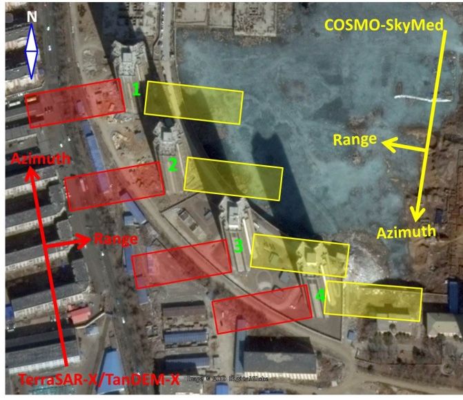
Thirty-six COSMO-SkyMed images acquired from 7 February 2015 to 10 July 2017 and nineteen
Thirty-six COSMO-SkyMed images acquired from 7 February 2015 to 10 July 2017 and nineteen
TerraSAR-X/TanDEM-X images acquired from 25 August 2015 to 5 October 2016 covering Shenyang
TerraSAR-X/TanDEM-X images acquired from 25 August 2015 to 5 October 2016 covering Shenyang
city are collected in this research. For TerraSAR-X/TanDEM-X, the satellites are orbiting the earth at
city are collected in this research. For TerraSAR-X/TanDEM-X, the satellites are orbiting the earth at the
the altitude of 514 km within an orbital tube of approximately 250 m radius [55,56]. On the other
altitude of 514 km within an orbital tube of approximately 250 m radius [55,56]. On the other hand,
hand, according to the COSMO-SkyMed mission and products description, the COSMO-SkyMed
according
satellitestoare
therunning
COSMO-SkyMed mission
within an orbital andthat
tube products description,
guarantees the within
a position COSMO-SkyMed satellites
+/−1000 m from a
arereference
runningground
withintrack
an orbital tube
[57]. The that guarantees
perpendicular a position
baseline within
distributions of +/−1000 m are
both stacks from a reference
depicted in
ground track [57]. The perpendicular baseline distributions of both stacks are depicted in Figure 9,Remote
Remote Sens. 2020, 12,
Sens. 2020, 12, 3100
x FOR PEER REVIEW 13
13 of
of 19
19
Figure 9, with perpendicular baseline apertures of approximately 2110.5 m (COSMO-SkyMed) and
with perpendicular baseline apertures of approximately 2110.5 m (COSMO-SkyMed) and 527.5 m
527.5 m (TerraSAR-X/TanDEM-X), respectively.
(TerraSAR-X/TanDEM-X), respectively.
(a) Perpendicular baselines of 36 COSMO-SkyMed images
(b) Perpendicular baselines of 19 TerraSAR-X images
Figure 9. Perpendicular baselines of COSMO-SkyMed and TerraSAR-X/TanDEM-X images.
TerraSAR-X/TanDEM-X images.
Since
Since the orbits
orbits are not
not uniformly
uniformly distributed, it is difficult to find realreal MRA
MRA orbits
orbits from
from both
both
stacks.
stacks. Instead,
Instead,MRA-like
MRA-likeorbits
orbitsare selected
are byby
selected keeping orbits
keeping close
orbits to normalized
close MRAMRA
to normalized positions. As a
positions.
result, ten out of thirty-six COSMO-SkyMed images and seven out of nineteen
As a result, ten out of thirty-six COSMO-SkyMed images and seven out of nineteen TerraSAR-X/TanDEM-X
images are selected. Theimages
TerraSAR-X/TanDEM-X detailed
areinformation
selected. Theof detailed
both stacks is given of
information in both
Tablestacks
2. According
is given toin
Equation
Table 2. (1), the elevation
According to resolution
Equation should
(1), the be 16.7 m for TerraSAR-X/TanDEM-X
elevation resolution should be and 16.75.1mm for
for
COSMO-SkyMed.
TerraSAR-X/TanDEM-X For comparison,
and 5.1 mtwo for different random orbit
COSMO-SkyMed. For configurations
comparison, two are also used for
different each
random
dataset in tomographic
orbit configurations arereconstruction, respectively.
also used for each dataset inThe random orbits
tomographic have equal respectively.
reconstruction, number of orbitsThe
with the MRA orbits, which are ten out of thirty-six for COSMO-SkyMed dataset and
random orbits have equal number of orbits with the MRA orbits, which are ten out of thirty-six for seven out of
nineteen for TerraSAR-X/TanDEM-X
COSMO-SkyMed dataset and seven dataset,
out respectively.
of nineteen Besides, the baseline apertures dataset,
for TerraSAR-X/TanDEM-X for the
random orbitsBesides,
respectively. are also identical to theapertures
the baseline MRA orbits,forwhich are approximately
the random orbits are 2110.5 m (COSMO-SkyMed)
also identical to the MRA
and 527.5
orbits, m (TerraSAR-X/TanDEM-X),
which are approximately 2110.5respectively.
m (COSMO-SkyMed) and 527.5 m (TerraSAR-X/TanDEM-X),
respectively.
Table 2. Parameters of the data stacks.
Table 2. Parameters of the data stacks.
Sensor TerraSAR-X/TanDEM-X COSMO-SkyMed
Sensor
Number of Images TerraSAR-X/TanDEM-X
19 COSMO-SkyMed
36
Number
Orbit of Images 19
Ascending 36
Descending
Orbit
Work Mode Ascending
StripMap Descending
StripMap
Altitude
Work Mode 514 km
StripMap 619.6 km
StripMap
Azimuth Resolution
Altitude 3.3
514mkm 619.63.0
km
Slant Azimuth
Range Resolution
Resolution 1.2 m
3.3 m 3.0 m
1.3
Incidence Angle (θ)
Slant Range Resolution 24.3
1.2 m 1.325.1
m
Baseline Aperture (∆b)
Incidence Angle ( )θ 527.5 m
24.3 2110.5
25.1 m
Elevation Resolution (ρs ) 16.7 m 5.1 m
Baseline Aperture ( Δb ) 527.5 m 2110.5 m
In this experiment, Longzhimeng Changyuan located in east Shenyang, with four high-rise
Elevation Resolution ( ρs ) 16.7 m 5.1 m
buildings of approximately 167 m is selected as our study area. The Google earth image and SAR
average amplitude images are shown in Figure 10. The COSMO-SkyMed and TerraSAR-X/TanDEM-X
In this experiment, Longzhimeng Changyuan located in east Shenyang, with four high-rise
buildings of approximately 167 m is selected as our study area. The Google earth image and SARYou can also read