Level set-based isogeometric topology optimization for maximizing fundamental eigenfrequency
←
→
Page content transcription
If your browser does not render page correctly, please read the page content below
Front. Mech. Eng.
https://doi.org/10.1007/s11465-019-0534-1

    RESEARCH ARTICLE

Manman XU, Shuting WANG, Xianda XIE

Level set-based isogeometric topology optimization for
maximizing fundamental eigenfrequency

© The Author(s) 2019. This article is published with open access at link.springer.com and journal.hep.com.cn

Abstract Maximizing the fundamental eigenfrequency                     [7] proposed the homogenization method. Homogeniza-
is an efficient means for vibrating structures to avoid                 tion is a material distribution method in which a design
resonance and noises. In this study, we develop an                     domain is discretized into small rectangular elements, and
isogeometric analysis (IGA)-based level set model for                  each element contains an artificial composite material with
the formulation and solution of topology optimization in               microscopic voids. The proposal of the homogenization
cases with maximum eigenfrequency. The proposed                        method was followed by a parallel exploration of the solid
method is based on a combination of level set method                   isotropic material with penalization (SIMP) method [8,9],
and IGA technique, which uses the non-uniform rational                 which uses an artificial isotropic material whose physical
B-spline (NURBS), description of geometry, to perform                  properties are expressed as a function of continuous
analysis. The same NURBS is used for geometry                          penalized material density (design variables). The phase-
representation, but also for IGA-based dynamic analysis                field method [10,11], which is also a material distribution
and parameterization of the level set surface, that is, the            method, is based on the theory of phase transitions. A
level set function. The method is applied to topology                  different type of method called evolutionary structural
optimization problems of maximizing the fundamental                    optimization (ESO) [12,13] has also been proposed. This
eigenfrequency for a given amount of material. A modal                 method eliminates elements with the lowest criterion value
track method, that monitors a single target eigenmode is               on the basis of certain heuristic criteria. ESO is
employed to prevent the exchange of eigenmode order                    computationally expensive because it requires a much
number in eigenfrequency optimization. The validity and                larger number of iterations with an enormous number of
efficiency of the proposed method are illustrated by                    intuitively generated solutions compared with material-
benchmark examples.                                                    based methods.
                                                                          However, these conventional TO methods, which are
Keywords topology optimization, level set method,                      based on element-wise design variables, suffer from
isogeometric analysis, eigenfrequency                                  numerical instability problems, such as checkerboards
                                                                       and mesh dependency. Accordingly, several studies have
                                                                       proposed prevention methods. The use of high-order
1    Introduction                                                      elements has been proven to be an effective means to
                                                                       prevent checkerboards [14,15], but this method entails a
Topology optimization (TO), which has been extensively                 considerable increase in computation time. Various filter
studied over the last decades, is a process of determining             techniques have been utilized to mitigate checkerboards
optimal layout of materials inside a given design domain.              and mesh dependency because these techniques require
TO has been applied to various structural optimization                 only a small amount of extra computation time and are
problems, such as minimum compliance [1,2] vibration                   simpler to implement than other methods [16,17]. Notably,
[3,4], and thermal issues [5,6], after Bendsøe and Kikuchi             filter schemes are purely heuristic. Other prevention
                                                                       schemes, such as perimeter control and gradient constraint,
                                                                       which often make the optimization procedure unstable, are
Received September 30, 2018; accepted November 11, 2018                yet to be improved.
                                                                          A new type of TO approach is the level set-based
                              ✉
Manman XU, Shuting WANG ( ), Xianda XIE
                                                                       method (LSM), which was developed by Sethian and
School of Mechanical Science and Engineering, Huazhong University of
Science and Technology, Wuhan 430074, China                            Wiegmann [18] to numerically track the motion of
E-mail: wangst@hust.edu.cn                                             structural boundaries. In LSM, boundaries are represented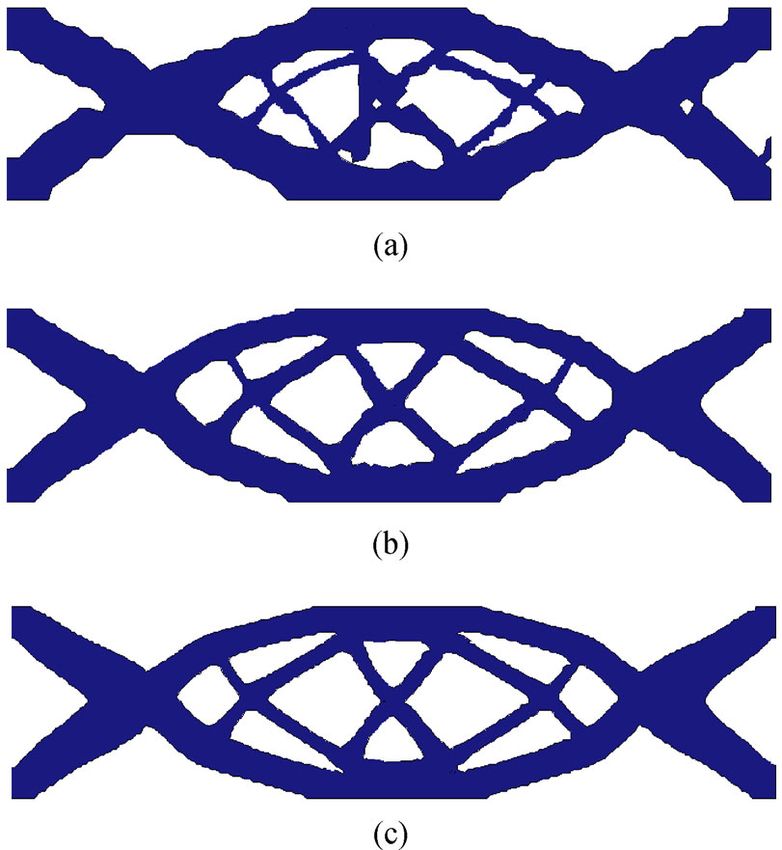
2                                                      Front. Mech. Eng.

as zero level set contour of an implicit high-dimensional       methods have been devised to help alleviate the difficulties
function (level set function or LSF), in which boundary         faced by IGA. Special parameterization techniques, such
motion, merging, and introduction of new holes are              as variational harmonic-based methods [29,30] and
performed. The evolution of a structural interface with         analysis-aware parameterization methods for single [31]
respect to time is tracked by solving a Hamilton-Jacobi         and multi-domain geometries [32], have been proposed for
(H-J) partial differential equation (PDE), where transport-     the computational domain. Alternatives to NURBS, such
ing LSF along its outward normal direction is equivalent to     as T-splines [33,34], polynomial splines over hierarchical
moving the boundaries along the descent gradient direc-         T-meshes (PHT-splines) [35–37], and Powell-Sabin splines
tion. The conventional level set-based TO approach uses         [38], have been studied for local refinement in IGA due to
shape derivatives coupled with the original LSM for             the limitation of the tensor product form of NURBS in
boundary tracking [19,20]. In this approach, regularization     computation refinement. Methods of parameterization of
that reinitializes LSF to be signed distance to a zero level    the interior domain while retaining the geometry exactness
set is employed to control the slope of LSF. This               from the CAD model have been devised [39,40], and
conventional approach is updated by solving the H-J             isogeometric collocation method is one of the most
equation via an explicit up-wind scheme [21,22]. Varia-         important among these methods [39]. With regard to
tions of the conventional approach include parameterizing       interior discretization obstacles, the isogeometric boundary
LSF using various basis functions, such as finite element        element method is a suitable candidate [41] because only
method (FEM) basis functions [23], radial basis functions       boundary data are required for analysis, and it enables
(RBFs) [24,25], and spectral parameterization [26], and         stress analysis [42], fracture analysis [43,44], acoustic
corresponding methods for solving the H-J equation. By          analysis [45], and shape optimization [46,47]. Considering
defining the interfaces between two material phases via the      that the integral efficiency of IGA is limited by the tensor
iso-contour of LSF, LSM can handle shape and topology           product structure of NURBS, an efficient quadrature rule,
changes during the optimization procedure and provides          which is more suitable for NURBS-based IGA compared
optimal structures with clear boundaries that are free of       with the Gaussian quadrature rule, has been proposed in
checkerboard patterns. Notably, most LSMs rely on finite         Ref. [48]. IGA has been applied to a wide range of
elements wherein boundaries are still represented by            problems, such as structural vibrations [49], fluid-structure
discretized mesh in the analysis field unless alternative        interaction [50,51], heat conduction analyses [52], shape
techniques are utilized to map the geometry to the analysis     optimization [53,54], shell analyses [55], TO [56], and
model.                                                          electromagnetics [57].
   Most of these TOs are performed in a fixed domain of             IGA-based shape optimization has been extensively
finite elements where FEM is used to solve optimization          investigated because remeshing is eliminated during the
problems. Currently used FEMs are often based on                optimization process. IGA has also been recently applied
Lagrange polynomials for analysis while the geometrical         to TO. The most commonly used TO approach is material
representation of structures relies on non-uniform rational     based, and the most commonly solved TO problem is the
B-splines (NURBS), which are the criteria in computer           minimum compliance case. In Ref. [58], TO was proposed
aided design (CAD) systems. Thus, conversion of                 based on isogeometric shape optimization. B-spline curves
NURBS-based representation into one that is compatible          were introduced to represent the material boundary, and the
with Lagrange polynomials, that is, mesh generation, is         coordinates of their control points were considered design
required in structural analysis. The disadvantages of FEM       variables. In Ref. [59], the trimmed spline surface
are as follows. First, the geometry approximation inherent      technique was used for spline-based TO. In Refs.
in the FEM mesh may generate an approximate error.              [60,61], optimality criteria (OC) and the method of moving
Second, frequent data interaction between geometry              asymptotes were implemented in the isogeometric-based
description and the computational mesh, which can be            SIMP method. In Ref. [62], the TO problem was solved by
found in several calculations (e.g., fluid, large deformation,   using a phase-field model, and IGA was utilized for the
and shape optimization problems), is cumbersome and             exact representation of the design domain. In Ref. [56],
error-prone. An integrating method, namely, isogeometric        IGA was introduced to a level set TO method, and NURBS
analysis (IGA) [27], for unifying analysis and CAD              basis functions were used for geometry description and
processes has been proposed to overcome these disadvan-         LSF parameterization.
tages. This method employs the same basis functions as a           Most studies on TO were restricted to compliance
technique for describing and analyzing the geometric            optimization, and the number of studies on TO of dynamic
model, which features the IGA method and CAD-based              problems is limited. Dynamic problems, such as vibration
parameterization of field variables in an isoparametric          and noise, are critical in many engineering fields, such as
manner. The first work on isogeometric approximation             aeronautical and automotive industries. As a typical
dates back to 1982 [28]; however, this method is                dynamic problem, structure vibration is controlled by the
considerably different from the IGA method. Several             structure’s dynamic characteristics, which are usually
Manman XU et al. LS-based isogeometric topology optimization for eigenvalue problem                       3

represented by the eigenfrequencies of the structure. Thus,     2.1   NURBS-based IGA
eigenfrequency optimization plays an important role in
improving dynamic characteristics.                              We assume that geometrical mapping Ψ maps the
   As an important research topic, eigenfrequency optimi-                          ^ into the physical domain Ω. Given
                                                                parameter domain Ω
zation has been studied by many scholars. Díaaz and
                                                                a knot vector Ξ ¼ ð1 ,2 ,:::,s Þ with a non-decreasing
Kikuchi [63] extended TO to eigenfrequency optimization
                                                                sequence of values lying in parameter space, the mapping
within the framework of the homogenization approach.
                                                                between two domains can be expressed as
Tenek and Hagiwara [64] introduced the SIMP method to
structural shape optimization and TO in eigenfrequency
problems. Xie and Steven [65] applied the ESO scheme to                                ^ ↓Ω, Ξ↕ ↓ΨðΞÞ:
                                                                                   Ψ : Ω↕                                    (1)
TO, and the specified eigenfrequency of the structure was           The NURBS curve is constructed by linear combina-
used as a constraint. Additional research has also been         tions of its basis functions, in which the coefficients are a
conducted on frequency optimization [66–70]. However,           given set of control points. A NURBS curve of p-degree is
standard density-based TO methods are unsuitable for            defined as
eigenfrequency optimization due to localized modes in
low-density areas [71]. Low-density areas are much more                                      X
                                                                                             n
flexible than areas with full densities; hence, they control                         ΨðÞ ¼          Ri,p ðÞPi ,             (2)
the lowest eigenmodes of the entire structure. By changing                                    i¼1
the penalization of stiffness in the SIMP method, a             where n ¼ s – p – 1 is the number of control points, Pi 2
modified algorithm has been proposed and applied to
                                                                ℝd is the ith control points in the physical domain, and
circumvent this numerical instability problem [3]. LSM
                                                                Ri,p ðÞ is the ith univariate NURBS basis function defined
that employs a crisp description of structure boundaries has
                                                                in the parameter space Ω   ^ as follows:
advantages over the density-based approach. The LSM
approach can avoid artificial modes localized in the weak
                                                                                               Ni,p ðÞωi
phase, which makes LSM a choice for eigenfrequency                                 Ri,p ðÞ ¼ X
                                                                                              n             ,                (3)
optimization. Many studies have been performed on level
                                                                                                 Ni,p ðÞωi
set TO for eigenfrequency problems [72–75].                                                   i¼1
   IGA-based TO has been extensively studied. However,
research on the combination of the level set approach and       where ωi 2 ð0,1Þ are non-decreasing weights associated
IGA is limited, and that on eigenfrequency problems is          with control points and Ni,p ðÞ represents the ith B-spline
absent. In this study, we develop a new optimization            basis functions of p-degree; it is defined by the following
method to formulate the TO problem for cases with               Cox-de Boor recursion formula [27].
maximum fundamental eigenfrequency by using LSM                  8            (
under the framework of IGA instead of conventional finite         >
                                                                 >               1 if i £ < iþ1
                                                                 >
                                                                 < Ni,0 ðÞ ¼
element analysis (FEA). Given that the OC algorithm is                           0 otherwise
particularly efficient for problems with many design                                                                          ,
                                                                 >
                                                                 >               – i               iþpþ1 –
variables and few constraints, we consider the OC method         >
                                                                 : Ni,p ðÞ ¼          N ðÞ þ                  N        ðÞ
for the solution of the optimization problem and conduct a                    iþp – i i,p–1      iþpþ1 – iþ1 iþ1,p–1
sensitivity analysis. The rest of this paper is organized as                                                                 (4)
follows. In Section 2, IGA and NURBS-based TO are
summarized. The eigenvalue optimization problem is              where basis function Ni,p ðÞ has its own support domain
described in Section 3, and the TO model is proposed in         ½i ,:::,iþpþ1  in which Ni,p ðÞ is non-zero. A knot vector is
Section 4. Section 5 presents numerical examples to             deemed open when the knots are repeated p þ 1 times at
demonstrate the validity of the proposed approach. The          the ends of the vector. In IGA, the open-knot vector is
conclusions and discussions are shown in Section 6.             generally used to satisfy the Kronecker delta property at
                                                                boundary points.
                                                                    A NURBS surface is a tensor product of bivariate
2   IGA for level set-based TO                                  NURBS curves in Ξ and H directions with p- and q-
                                                                degrees, respectively, where a knot vector H ¼ ðη1 ,η2 ,:::,
In IGA, geometric modeling and analysis are integrated by       ηt Þ is given in H direction.
using NURBS, where the basis function is a bridge of the
                                                                                          X
                                                                                          n X
                                                                                            m
parameter domain, physical field, and numerical solution.                       Ψð,ηÞ ¼              Rp,q
                                                                                                      i,j ð,ηÞPi,j ,        (5)
In the proposed method, we consider the NURBS basis                                        i¼1 j¼1
function as a bound between IGA and parameterized LSM.
We provide a brief review of IGA and NURBS-                     where m ¼ t – q – 1, Pi,j are control points and Rp,q
                                                                                                                  i,j are
parameterized LSM.                                              bivariate basis functions of the form: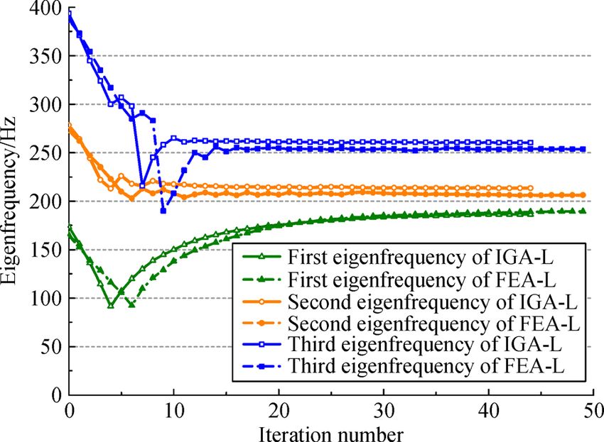
4 Front. Mech. Eng.
Ni,p ðÞNj,q ðηÞωi,j ε ¼ Bu: (9)
Rp,q
i,j ¼ X
n Xm , (6)
Ni,p ðÞNj,q ðηÞωi,j
i¼1 j¼1 2.2 NURBS-based parameterized LSM
where Ni,p ðÞ and Nj,q ðηÞ are B-spline basis functions LSM is a TO method that implicitly defines the interfaces
defined on the knot vector Ξ ¼ ð1 ,2 ,:::,s Þ and between material and void phases by iso-contours of a
H ¼ ðη1 ,η2 ,:::,ηt Þ, respectively. The interval Ξ H forms high-dimensional LSF. Thus, this method allows a crisp
a patch containing all elements, namely, ½k ,kþ1 description of the material boundary and helps avoid mesh-
½ηl ,ηlþ1 , 1£k£n þ p, and 1£l£m þ q, which are dependent problems.
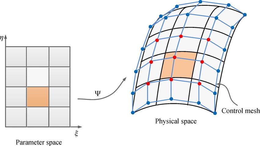
defined by the two knot vectors. The parameter domain The shape of the interpolating functions of LSF directly
and corresponding physical domain for a surface model are influences the smoothness of LSF and the material domain.
depicted in Fig. 1. In its most general form, LSF is described by a summation
On the basis of the isoparametric concept, the IGA of interpolating functions scaled by their degree of freedom
approach utilizes the same parameters for geometry and (DOF).
analysis models, and the basis functions used for geometry
representation are also employed to approximate the X
N
numerical solution of PDEs. With Eq. (2), the numerical ΦðxÞ ¼ fT ðxÞs ¼ fi ðxÞsi , (10)
solution u can be expressed as i
X
n where x denotes the spatial coordinate, fi comprises
u¼ Ri ðÞui , (7) interpolating functions associated with N spatial points,
i¼1 and si are time-dependent optimization variables.
The most commonly used interpolation functions in
where Ri is the ith basis function. ui , which is referred to as
present LSM are FEM shape functions and RBFs, and their
a control variable at the ith control point, is the coefficient
corresponding optimization variables are nodal values and
used to approximate the field variable u, which plays the
expansion coefficients, respectively. We introduce NURBS
same role as the nodal value in FEA. For each element, the
basis functions, which can be used to approximate a given
shape function and strain-displacement matrix can be
set of points with smooth polynomial functions, for
expressed as
parameterizing LSF. Thus, the NURBS-based parameteri-
R ¼ ½R1 R2 :::Rn , zed LSF is constructed as
2 3 X
N
∂R1 ∂Rn
0 ::: 0 7 ΦðxÞ ¼ RT s ¼ Ri ðxÞsi , (11)
6 ∂x ∂x
6 7 i
6 ∂R1 ∂Rn 7
B¼6
6 0 ::: 0 7: (8)
6 ∂y ∂y 7
7
where Ri is the ith NURBS basis function and si is the ith
4 ∂R1 ∂R1 ∂Rn ∂Rn 5 time-dependent expansion coefficient related to the ith
::: control point.
∂y ∂x ∂y ∂x
The evolution of LSF is governed by the following H-J
The strain matrix is given by equation.
Fig. 1 Geometrical mapping Ψ maps the common parameter space ð,ηÞ onto the physical space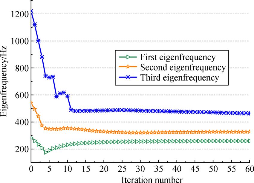
Manman XU et al. LS-based isogeometric topology optimization for eigenvalue problem                  5

                  ∂Φðx,tÞ      dx                                material, and HðΦÞ is the Heaviside function, which takes
                          þ rΦ    ¼ 0,                   (12)    0 for Φ < 0 and 1 otherwise.
                    ∂t         dt
                                                                    The eigenvalue problem has a family of solutions lk and
where t denotes pseudo-time, which represents the                uk , k³1. The first eigenfrequency and its eigenvector are
evolution of the design in the optimization process. The         related to each other as
speed of movement of a point on the level set surface can                        0                               1
be expressed by V ¼ dx=dt. V n ¼ V ⋅n defines the speed
                                                                                 B  ! Dijkl εkl ðuÞεij ðvÞHðΦÞdΩ
                                                                                                                 C
of propagation of all level sets along the external normal             l1 ¼ min@ Ω                               A:    (19)
velocity, where n ¼ – rΦ=jrΦj. Therefore, Eq. (12) can
be rewritten as
                                                                                          !Ω  uvHðΦÞdΩ

                     ∂Φðx,tÞ
                             ¼ V n jrΦj:                 (13)    3.2   Optimization model
                       ∂t
  By substituting Eq. (11) into Eq. (13), the H-J equation       We consider the TO problem by maximizing the first
can be written as                                                eigenfrequency under a volume constraint. Under the
                                                                 NURBS-based level set framework, eigenfrequency TO
                     ∂s                                          can be expressed as
                RT      þ V n ⋅jðrRÞT sj ¼ 0:            (14)
                     ∂t
                                                                             Maximize J ðu,ΦÞ ¼ l1
  The moving speed of the material free boundary during
evolution is related to the time derivative of the expansion                 subject to : aðu,v,ΦÞ ¼ l1 bðu,v,ΦÞ,
coefficient as follows:                                                                                                   (20)
                                                                                          !ΩHðΦÞdΦ£Vmax,
                                RT    ∂s                                                  smin £si £smax ,
                   Vn ¼ –          T ∂t :                (15)
                             jðrRÞ sj
                                                                 where J ðu,ΦÞ is the objective function, Vmax represents the
                                                                 maximum admissible volume of the design domain, and
                                                                 smin and smax stand for the lower and upper bounds of the
3 Optimization problems of maximizing                            design variables, respectively.
eigenvalue                                                          However, in the eigenfrequency optimization process,
                                                                 the value of higher-order eigenfrequency may decrease
3.1   Definition of the eigenvalue problem                        whereas that of lower-order target eigenfrequency may
                                                                 increase, which may possibly lead to the repetition and
We describe the eigenvalue problems in the linear elastic        exchange of mode order number. Given that the objective
continuum to facilitate the computation of vibration             and constraint functions are typically defined based on a
frequencies and modes. A linear elastic continuum                fixed modal order, the sensitivities of these functions are
structure with a constant mass density is defined in domain       discontinuous in the repeated eigenfrequency case.
Ω  ℝd ðd ¼ 2 or 3Þ with the boundary Γ ¼ ∂Ω. The                Approaches are often used to maintain the simplicity of
weak formulation of the undamped free vibration problem          eigenfrequency during the entire optimization process and
can be expressed as                                              overcome this ill-posed problem. The modal assurance
                                                                 criterion (MAC) method, an efficient and accurate strategy,
               aðu,vÞ – lbðu,vÞ ¼ 0, v 2 U ,             (16)    is introduced to monitor a single target mode, which is the
where eigenfrequency l and corresponding eigenvector u,          first mode in this study. The definition of MAC is
that is, the displacement subdomain in Ω, are solutions of                                            juTa ub j2
this eigenvalue problem, v is adjoint displacement, which                       MACðua ,ub Þ ¼                       ,   (21)
                                                                                                  ðuTa ua ÞðuTb ub Þ
satisfies the kinematic boundary condition, and U is a
space of kinematically admissible displacement fields. In         where ua and ub represent two eigenvectors: One is the
LSM, að⋅,⋅Þ and bð⋅,⋅Þ are respectively defined as                reference eigenvector of the current optimization cycle and
                                                                 the other is the objective eigenvector of the previous cycle
         aðu,v,ΦÞ ¼    !ΩDijkl εkl ðuÞεijðvÞHðΦÞdΩ,      (17)    in the eigenvalue optimization process. The value of MAC
                                                                 varies between 0 and 1. Theoretically, a MAC value of 1
                                                                 means that the two eigenvectors representing modal shapes
               bðu,v,ΦÞ ¼    !ΩuvHðΦÞdΩ,                (18)    are exactly the same. However, this condition is impossible
                                                                 because the structural configuration changes in each
where Dijkl stands for the elasticity tensor component, εij is   iteration, and the modal shapes of adjacent iterations are
the strain tensor component,  is the density of the             not orthogonal to each other. By comparing a few reference
6 Front. Mech. Eng.
eigenvectors with an objective eigenvector uobj , a new aðu# ,v,ΦÞ – l1 bðu# ,v,ΦÞ ¼ 0, (27)
objective eigenvector is obtained in each iteration step of
the optimization process, and it can be expressed as aðu,v# ,ΦÞ – l1 bðu,v# ,ΦÞ ¼ 0, (28)
unobj ¼ unk that max½MACðuobj ,uk Þ,
n–1 n
k
1 – bðu,v,ΦÞ ¼ 0: (29)
k ¼ 1,2,:::,Nm , (22) Given that the real mode u is equal to the adjoint mode v,
where Nm is the number of modal eigenvectors that need to Eq. (29) is a normalization condition for the eigenvector. In
be checked, superscript of displacement indicates the this case, Eq. (24) can be simplified as
number of iteration step, that is, in the nth iteration, ∂Lðu,ΦÞ
objective eigenvector of previous iteration step uobj
n–1
is used ∂t
¼ !Ω
FðuÞ þ Λ δðΦÞjrΦjV n dΩ, (30)
to calculate the MAC value.
where FðuÞ ¼ Dijkl εðuÞεðuÞ – l1 uu. By substituting Eqs.
3.3 Sensitivity analysis (11) and (15) into the preceding shape derivative equation,
we obtain
Establishing the relationship between the optimization ∂Lðu,ΦÞ ∂s
function and design variables by using a sensitivity
∂t
¼ – !
Ω
FðuÞ þ Λ δðΦÞR dΩ:
∂t
(31)
analysis approach is necessary to solve the optimization
problem. According to the material derivative and the Given that
adjoint method, the Lagrangian function can be defined as
∂Lðu,ΦÞ ∂J ðu,ΦÞ ∂V ðu,ΦÞ ∂Lðu,ΦÞ ∂s
¼ þΛ ¼ , (32)
Lðu,ΦÞ ¼ J ðu,ΦÞ þ aðu,v,ΦÞ – l1 bðu,v,ΦÞ ∂s ∂s ∂s ∂s ∂t
the sensitivity of the objective function and volume
þΛ !Ω
HðΦÞdΦ – Vmax , (23) constraint with respect to the design variables is respec-
tively obtained as follows:
where Λ is the Lagrangian multiplier. Assuming that ∂J ðu,ΦÞ
V ðu,ΦÞ ¼ !Ω HðΦÞdΦ – Vmax is the volume constraint, the ∂s
¼ – !ΩFðuÞδðΦÞRdΩ, (33)
shape derivative of Lagrangian function Lðu,ΦÞ is
∂V ðu,ΦÞ
∂Lðu,ΦÞ
¼ l#1 þ a# ðu,v,ΦÞ – l1 b# ðu,v,ΦÞ ∂s
¼ – !ΩδðΦÞRdΩ: (34)
∂t
– l#1 bðu,v,ΦÞ þ ΛV # ðu,ΦÞ, (24)
4 Numerical implementation
where the material derivatives of aðu,v,ΦÞ and bðu,v,ΦÞ
are respectively given by Many design variables, which correspond to large-scale
nonlinear equations in the eigenvalue problem, exist in
a# ðu,v,ΦÞ ¼ !Ω Dijkl εkl ðu#ÞεijðvÞHðΦÞdΩ continuum structural TO. Thus, OC is introduced to solve this
eigenvalue TO problem. By properly iterating and updating
þ !ΩDijkl εkl ðu#Þεijðv#ÞHðΦÞdΩ the design variables, this optimization problem is guaranteed
to converge to a final solution. Starting from an initial value,
the iterative formula of the design variables is expressed as
þ !ΩDijkl εkl ðu#ÞεijðvÞδðΦÞjrΦjV ndΩ, (25)
si
ðkþ1Þ ðkÞ ðkÞ
¼ ci si : (35)
ðkÞ
b# ðu,v,ΦÞ ¼ !Ωu#vHðΦÞdΩ þ !Ωuv#HðΦÞdΩ Theoretically, the iteration coefficients ci are obtained
by setting Eq. (32) equal to 0, which can be written as
( )
þ !ΩuvδðΦÞjrΦjV ndΩ, (26) ðkÞ
ci ¼ –
∂J ðu,ΦÞ
=max ,Λ ðkÞ ∂V ðu,ΦÞ
, (36)
ðkÞ ðkÞ
∂si ∂si
where u# and v# are partial derivatives of u and v,
respectively, with respect to pseudo-time. δðxÞ is the Dirac where is a very small number that can avoid singularity
function. when the sensitivity of the volume constraint with respect
The adjoint state equation can be obtained by the Kuhn- to the design variables is equal to 0. The Lagrangian
Tucker condition. multiplier Λ is calculated by the bisection method [76].Manman XU et al. LS-based isogeometric topology optimization for eigenvalue problem 7
A flowchart of the structural TO for maximization of the enforces these conditions to be satisfied pointwise. Given
first eigenfrequency problem is depicted in Fig. 2. Given that NURBS basis functions associated with the interior
the condition of constraints, when the relative difference control points vanish at the structural boundary when
value of the objective function in the current and previous open-knot vectors are employed, the displacement boun-
iterations is less than 10–3, this optimization process is dary condition applied on the left and right sides of the
considered convergent, and the current optimization beam is imposed by setting the displacement values at left
process is terminated. and right boundary control points to zero. All results are
produced with programs developed in the MATLAB
R2018a environment on a computer with an Intel Core
5 Numerical examples i3-3240 CPU, 3.4 GHz clock speed, and 6 GB RAM.
Additional details on the implementation of IGA on the
In this section, the proposed IGA-based level set TO MATLAB platform were presented in Ref. [77].
framework is applied to two 2D optimization problems.
For all examples, the properties of the isotropic material 5.1 Cantilever beam
are set as follows: Young’s modulus E ¼ 210 GPa and
mass density ¼ 7:8 103 kg=m3 . The properties of the The first numerical example of a short cantilever beam for
artificial weak material are E0 ¼ 210 10 – 3 GPa and maximizing the first eigenfrequency optimization problem
mass density ¼ 7:8 10 – 3 kg=m3 . Poisson’s ratio ¼ is shown in Fig. 3. The entire design domain is a rectangle
0:3 and plane stress state are assumed for all the materials. with a size of 0.2 m0.1 m, a Dirichlet boundary, and fixed
The two examples are TO of maximizing the fundamental displacement at the left edge of the design domain. A
eigenfrequency of the plane structure with a unit thickness concentrated nonstructural mass M ¼ 15:6 kg that is one-
of 0:001 m and a prescribed material volume fraction of tenth of the total structural mass of the plate is placed at the
α ¼ 50%. In the initial design, the available material is center of the right side. Notably, the structure disappears
uniformly distributed over the entire admissible design without the nonstructural mass because no structure leads
domain. In the following examples, the boundary condi- to the highest eigenfrequencies.
tions are imposed by the collocation method, which In this example, IGA- and FEA-based TO approaches
Fig. 2 Flowchart of the optimization procedure8 Front. Mech. Eng.
quarter of FEM) when the element number is sufficiently
large. Table 1 shows that the computation efficiency of
IGA-based LSM is higher than that of FEM-based LSM in
TO due to the fewer DOFs or smaller size of equations in
the IGA-based approach. However, because of the extra
calculations of the basis functions and their derivative in
the IGA-based approach, the ratio between the iteration
time and DOFs of the IGA-based optimization method is
higher than that of the FEM-based method.
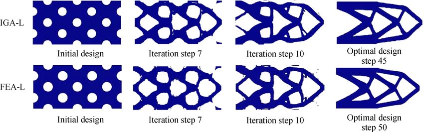
Fig. 3 Design domain of a cantilever beam structure The optimal layouts obtained by using IGA and FEA
with 12864 elements are shown in Fig. 4. In this case, the
are applied to a similar problem for comparison. For this results are similar, and the crisp boundary is obtained due
2D example, equally spaced open-knot vectors are used for to the level set method. Adopting B-spline basis functions
x and y directions, and the degrees of NURBS basis to parameterize the level set function together with IGA for
functions on the two directions are the same, i.e., calculation instead of FEA leads to the rapid convergence
p ¼ q ¼ 2. Nine-node quadratic rectangle elements are of the IGA-based optimization process.
used for FEA, and the element number of both methods is The convergence history of optimization using IGA and
the same, which facilitates a comparison under identical FEA with 128 64 elements is shown in Figs. 5 and 6.
conditions. Figure 5 shows the convergence history of the first
The computation consumption times of the two methods eigenfrequency and volume ratio of the structure by
are shown in Table 1. Notably, for simplicity in the using IGA- and FEA-based optimization frameworks,
proceeding table and figures, IGA-L and FEM-L represent respectively. The initial designs and resultant structures of
IGA- and FEM-based LSM, respectively. The solution both methods are basically the same. In optimization with
time of the system equation includes the time spent on the IGA method, the ωi of the initial design and the
assembling the stiffness matrix and solving the equation to resultant optimum are 173.5 and 188.7, respectively. The
obtain an objective function. In this case, when the volume ratio of the initial design and the resultant optimum
numbers of Lagrange and NURBS elements are a b (a are 0.79 and 0.5, respectively. Thus, the fundamental
and b represent the number of elements in x and y eigenfrequency increased by 8.8% and the volume
directions, respectively), the number of DOFs of the IGA- decreased by 36.7%. Figure 6 shows the iteration history
based method is ða þ 2Þðb þ 2Þ ¼ ab þ 2a þ 2b þ 4 and of the first three eigenfrequencies by using both methods.
that of FEM is ð2a þ 1Þð2b þ 1Þ ¼ 4ab þ 2a þ 2b þ 1. The first eigenfrequency always remains simple, whereas
The DOF of IGA is much less than that of FEM (nearly a the second and third eigenfrequencies tend to oscillate and
Table 1 Comparison of IGA- and FEA-based LSM TO
Method Number of elements Number of DOFs Time of each iteration/s Time of solution of system equation/s
IGA-L 256128 67080 873.26 713.68
FEA-L 256128 263682 1580.42 1237.16
IGA-L 12864 17160 30.06 25.31
FEA-L 12864 66306 54.17 43.97
IGA-L 6432 4488 6.41 5.18
FEA-L 6432 16770 8.55 6.85
Fig. 4 Optimized results obtained by using IGA and FEA methods with 128 64 elementsManman XU et al. LS-based isogeometric topology optimization for eigenvalue problem 9
Fig. 7 Design domain of a clamped beam structure
The degree of NURBS basis function is 2 in both
directions. The resulting layouts shown in Fig. 8 indicate
that the mesh dependency problem is avoided in the
proposed method. This figure also shows that an inaccurate
Fig. 5 Comparison of IGA and FEA in terms of convergence
optimum topology with a rough boundary is obtained as a
history
consequence of coarse meshes. By refining the mesh, the
smoothness of the boundaries of the optimal layout is
improved. However, when the number of elements is larger
than 12832, the resulting layout slightly changes.
Accounting for the computation cost and precision of
results, 12832 meshes are used in this example.
Fig. 6 Comparison of IGA and FEA in terms of eigenfrequency
history
overlap. By using the MAC method, problems regarding
the orders of eigenfrequency exchange during the
optimization process are avoided. The first eigenfrequency
generally increases, and the second and third eigenfre-
quencies decrease as the volume ratio decreases.
Fig. 8 Optimal layouts obtained by using (a) 6416 meshes,
5.2 Beam with clamped ends (b) 12832 meshes, and (c) 25664 meshes
In this section, we present an example of maximizing the The convergence history of the objective function and
fundamental frequency of a clamped beam structure shown volume ratio is given in Fig. 9. The first eigenfrequency of
in Fig. 7. The working domain has a size of 0.4 m0.1 m. the initial design and the resultant topology are 244.3 and
A fixed displacement boundary condition is imposed on 257.4, respectively. The volume ratio of the initial design
both sides, and a concentrated nonstructural mass M = 31.2 and the resultant topology are 0.82 and 0.5, respectively.
kg is placed at the center of structure. In this example, the Thus, the fundamental frequency increases by 5.4%, and
capability of the proposed method to capture the optimum the volume decreases by 39%. Figure 10 shows the
topology and the effect of the number of elements are convergence history of the first three eigenfrequencies. The
studied. For this purpose, a clamped beam is solved with fundamental frequency remains simple throughout the
three mesh sizes, namely, 6416, 12832, and 25664. entire optimization process. The value of first eigenfre-10 Front. Mech. Eng.
of maximizing the fundamental eigenfrequency, a regulari-
zation method for the repetition or exchange of eigen-
frequencies was employed to guarantee the simple
behavior of structural eigenfrequency.
Two benchmark numerical examples of TO for dynamic
problems were applied to verify the validity of the
proposed approach. The results obtained from the
comparison of FEA- and IGA-based level set TO methods
demonstrated that the proposed IGA-based optimization
method has better computational efficiency and converges
faster than the traditional FEA-based optimization method.
The results also showed that solving dynamic TO problems
by using IGA together with the level set method is
possible. Although we only presented examples of 2D
structures, no theoretical difficulties will be encountered if
Fig. 9 Convergence history
the proposed is extended to the optimization of 3D
structures.
Acknowledgements This research was supported by the National Natural
Science Foundation of China (Grant No. 51675197).
Open Access This article is licensed under a Creative Commons
Attribution 4.0 International License, which permits use, sharing, adaptation,
distribution and reproduction in any medium or format, as long as you give
appropriate credit to the original author(s) and the source, provide a link to the
Creative Commons licence, and indicate if changes were made.
The images or other third party material in this article are included in the
article’s Creative Commons licence, unless indicated otherwise in a credit
line to the material. If material is not included in the article’s Creative
Commons licence and your intended use is not permitted by statutory
regulation or exceeds the permitted use, you will need to obtain permission
directly from the copyright holder.
To view a copy of this licence, visit http://creativecommons.org/licenses/
by/4.0/.
Fig. 10 Iteration history of the first three eigenfrequencies
References
quency gradually increases after the fifth iteration, whereas
that of the second and third eigenfrequencies decline with 1. Suzuki K, Kikuchi N. A homogenization method for shape and
the increase in iterations. topology optimization. Computer Methods in Applied Mechanics
and Engineering, 1991, 93(3): 291–318
2. Sigmund O. A 99 line topology optimization code written in Matlab.
6 Conclusions Structural and Multidisciplinary Optimization, 2001, 21(2): 120–
127
We solved maximum fundamental eigenfrequency TO 3. Pedersen N L. Maximization of eigenvalues using topology
problems with a level set model based on the IGA optimization. Structural and Multidisciplinary Optimization, 2000,
technique. IGA combines the fundamental idea of FEM 20(1): 2–11
with the spline technique from a computer-aided geometry 4. Du J, Olhoff N. Minimization of sound radiation from vibrating bi-
design for the integration of CAD and CAE. The IGA material structures using topology optimization. Structural and
method was also introduced to TO due to its superiority Multidisciplinary Optimization, 2007, 33(4–5): 305–321
over currently used FEM in terms of accuracy and 5. Iga A, Nishiwaki S, Izui K, et al. Topology optimization for thermal
efficiency. The feature of the proposed method is the conductors considering design-dependent effects, including heat
combination of IGA and LSM in eigenfrequency optimi- conduction and convection. International Journal of Heat and Mass
zation where the same basis functions (NURBS) are used Transfer, 2009, 52(11–12): 2721–2732
for geometry representation, dynamic analysis, and para- 6. Yamada T, Izui K, Nishiwaki S. A level set-based topology
meterization of the implicit LSF. High accuracy and optimization method for maximizing thermal diffusivity in problems
smoothness of LSF were achieved by using smooth including design-dependent effects. Journal of Mechanical Design,
NURBS basis functions to approximate LSF. In the case 2011, 133(3): 031011Manman XU et al. LS-based isogeometric topology optimization for eigenvalue problem 11
7. Bendsøe M P, Kikuchi N. Generating optimal topologies in 25. Luo Z, Tong L, Wang M Y, et al. Shape and topology optimization
structural design using a homogenization method. Computer of compliant mechanisms using a parameterization level set method.
Methods in Applied Mechanics and Engineering, 1988, 71(2): Journal of Computational Physics, 2007, 227(1): 680–705
197–224 26. Gomes A A, Suleman A. Application of spectral level set
8. Bendsøe M P. Optimal shape design as a material distribution methodology in topology optimization. Structural and Multi-
problem. Structural Optimization, 1989, 1(4): 193–202 disciplinary Optimization, 2006, 31(6): 430–443
9. Rozvany G I N, Zhou M, Birker T. Generalized shape optimization 27. Hughes T J R, Cottrell J A, Bazilevs Y. Isogeometric analysis: CAD,
without homogenization. Structural Optimization, 1992, 4(3–4): finite elements, NURBS, exact geometry and mesh refinement.
250–252 Computer Methods in Applied Mechanics and Engineering, 2005,
10. Bourdin B, Chambolle A. Design-dependent loads in topology 194(39–41): 4135–4195
optimization. ESAIM. Control, Optimisation and Calculus of 28. Grebennikov A I. Isogeometric approximation of functions of one
Variations, 2003, 9: 19–48 variable. USSR Computational Mathematics and Mathematical
11. Wang M Y, Zhou S. Phase field: A variational method for structural Physics, 1982, 22(6): 42–50
topology optimization. Computer Modeling in Engineering & 29. Nguyen T, Jüttler B. Parameterization of contractible domains using
Sciences, 2004, 6(6): 547–566 sequences of harmonic maps. In: Proceedings of International
12. Xie Y M, Steven G P. A simple evolutionary procedure for Conference on Curves and Surfaces. Berlin: Springer, 2010, 501–
structural optimization. Computers & Structures, 1993, 49(5): 885– 514
896 30. Xu G, Mourrain B, Duvigneau R, et al. Constructing analysis-
13. Querin O M, Steven G P, Xie Y M. Evolutionary structural suitable parameterization of computational domain from CAD
optimisation (ESO) using a bidirectional algorithm. Engineering boundary by variational harmonic method. Journal of Mathematical
Computations, 1998, 15(8): 1031–1048 Physics, 2013, 252: 275–289
14. Díaz A, Sigmund O. Checkerboard patterns in layout optimization. 31. Xu G, Mourrain B, Duvigneau R, et al. Optimal analysis-aware
Structural Optimization, 1995, 10(1): 40–45 parameterization of computational domain in isogeometric analysis.
15. Jog C S, Haber R B. Stability of finite element models for In: Proceedings of International Conference on Geometric Modeling
distributed-parameter optimization and topology design. Computer and Processing. Berlin: Springer, 2010, 236–254
Methods in Applied Mechanics and Engineering, 1996, 130(3–4): 32. Xu G, Mourrain B, Duvigneau R, et al. Analysis-suitable volume
203–226 parameterization of multi-block computational domain in isogeo-
16. Sigmund O. Materials with prescribed constitutive parameters: An metric applications. Computer-Aided Design, 2013, 45(2): 395–
inverse homogenization problem. International Journal of Solids 404
and Structures, 1994, 31(17): 2313–2329 33. Bazilevs Y, Calo V M, Cottrell J A, et al. Isogeometric analysis
17. Petersson J, Sigmund O. Slope constrained topology optimization. using T-splines. Computer Methods in Applied Mechanics and
International Journal for Numerical Methods in Engineering, 1998, Engineering, 2010, 199(5–8): 229–263
41(8): 1417–1434 34. Wu Z, Huang Z, Liu Q, et al. A local solution approach for adaptive
18. Sethian J A, Wiegmann A. Structural boundary design via level set hierarchical refinement in isogeometric analysis. Computer Methods
and immersed interface methods. Journal of Computational Physics, in Applied Mechanics and Engineering, 2015, 283: 1467–1492
2000, 163(2): 489–528 35. Nguyen-Thanh N, Kiendl J, Nguyen-Xuan H, et al. Rotation free
19. Osher S J, Santosa F. Level set methods for optimization problems isogeometric thin shell analysis using PHT-splines. Computer
involving geometry and constraints: I. Frequencies of a two-density Methods in Applied Mechanics and Engineering, 2011, 200(47–
inhomogeneous drum. Journal of Computational Physics, 2001, 48): 3410–3424
171(1): 272–288 36. Nguyen-Thanh N, Nguyen-Xuan H, Bordas S P A, et al.
20. Allaire G, Jouve F, Toader A M. A level-set method for shape Isogeometric analysis using polynomial splines over hierarchical
optimization. Mathematical Rendering, 2002, 334(12): 1125–1130 T-meshes for two-dimensional elastic solids. Computer Methods in
(in French) Applied Mechanics and Engineering, 2011, 200(21–22): 1892–
21. Wang M Y, Wang X, Guo D. A level set method for structural 1908
topology optimization. Computer Methods in Applied Mechanics 37. Atroshchenko E, Tomar S, Xu G, et al. Weakening the tight coupling
and Engineering, 2003, 192(1–2): 227–246 between geometry and simulation in isogeometric analysis: From
22. Allaire G, Jouve F, Toader A M. Structural optimization using sub- and super-geometric analysis to geometry-independent field
sensitivity analysis and a level-set method. Journal of Computa- approximation (GIFT). International Journal for Numerical Methods
tional Physics, 2004, 194(1): 363–393 in Engineering, 2018, 114(10): 1131–1159
23. Dijk N P, Langelaar M, Keulen F. Explicit level-set-based topology 38. Speleers H, Manni C, Pelosi F, et al. Isogeometric analysis with
optimization using an exact Heaviside function and consistent Powell-Sabin splines for advection-diffusion-reaction problems.
sensitivity analysis. International Journal for Numerical Methods in Computer Methods in Applied Mechanics and Engineering, 2012,
Engineering, 2012, 91(1): 67–97 221–222: 132–148
24. Wang S, Wang M Y. Radial basis functions and level set method for 39. Auricchio F, Da Veiga L B, Hughes T J R, et al. Isogeometric
structural topology optimization. International Journal for Numeri- collocation methods. Mathematical Models and Methods in Applied
cal Methods in Engineering, 2006, 65(12): 2060–2090 Sciences, 2010, 20(11): 2075–210712 Front. Mech. Eng.
40. Xu G, Li M, Mourrain B, et al. Constructing IGA-suitable planar Applied Mechanics and Engineering, 2009, 198(49–52): 3902–
parameterization from complex CAD boundary by domain partition 3914
and global/local optimization. Computer Methods in Applied 56. Wang Y, Benson D J. Isogeometric analysis for parameterized LSM-
Mechanics and Engineering, 2018, 328: 175–200 based structural topology optimization. Computational Mechanics,
41. Simpson R N, Bordas S P, Trevelyan J, et al. A two-dimensional 2016, 57(1): 19–35
isogeometric boundary element method for elastostatic analysis. 57. Buffa A, Sangalli G, Vázquez R. Isogeometric analysis in
Computer Methods in Applied Mechanics and Engineering, 2012, electromagnetics: B-splines approximation. Computer Methods in
209–212: 87–100 Applied Mechanics and Engineering, 2010, 199(17–20): 1143–
42. Lian H, Simpson R N, Bordas S. Stress analysis without meshing: 1152
Isogeometric boundary-element method. Proceedings of the Institu- 58. Lee S, Kwak B M, Kim I Y. Smooth boundary topology
tion of Civil Engineers: Engineering and Computational Mechanics, optimization using B-spline and hole generation. International
2013, 166(2): 88–99 Journal of CAD/CAM, 2007, 7(1): 11–20
43. Peng X, Atroshchenko E, Kerfriden P, et al. Isogeometric boundary 59. Seo Y D, Kim H J, Youn S K. Isogeometric topology optimization
element methods for three dimensional static fracture and fatigue using trimmed spline surfaces. Computer Methods in Applied
crack growth. Computer Methods in Applied Mechanics and Mechanics and Engineering, 2010, 199(49–52): 3270–3296
Engineering, 2017, 316: 151–185 60. Hassani B, Khanzadi M, Tavakkoli S M. An isogeometrical
44. Peng X, Atroshchenko E, Kerfriden P, et al. Linear elastic fracture approach to structural topology optimization by optimality criteria.
simulation directly from CAD: 2D NURBS-based implementation Structural and Multidisciplinary Optimization, 2012, 45(2): 223–
and role of tip enrichment. International Journal of Fracture, 2017, 233
204(1): 55–78 61. Tavakkoli S M, Hassani B, Ghasemnejad H. Isogeometric topology
45. Simpson R N, Scott M A, Taus M, et al. Acoustic isogeometric optimization of structures by using MMA. International Journal of
boundary element analysis. Computer Methods in Applied Optimization in Civil Engineering, 2013, 3(2): 313–326
Mechanics and Engineering, 2014, 269: 265–290 62. Dedè L, Borden M J, Hughes T J R. Isogeometric analysis for
46. Lian H, Kerfriden P, Bordas S P A. Shape optimization directly from topology optimization with a phase field model. Archives of
CAD: An isogeometric boundary element approach using T-splines. Computational Methods in Engineering, 2012, 19(3): 427–465
Computer Methods in Applied Mechanics and Engineering, 2017, 63. Díaaz A R, Kikuchi N. Solutions to shape and topology eigenvalue
317: 1–41 optimization problems using a homogenization method. Interna-
47. Lian H, Kerfriden P, Bordas S P. Implementation of regularized tional Journal for Numerical Methods in Engineering, 1992, 35(7):
isogeometric boundary element methods for gradient-based shape 1487–1502
optimization in two-dimensional linear elasticity. International 64. Tenek L H, Hagiwara I. Static and vibrational shape and topology
Journal for Numerical Methods in Engineering, 2016, 106(12): optimization using homogenization and mathematical program-
972–1017 ming. Computer Methods in Applied Mechanics and Engineering,
48. Hughes T J R, Reali A, Sangalli G. Efficient quadrature for NURBS- 1993, 109(1–2): 143–154
based isogeometric analysis. Computer Methods in Applied 65. Xie Y M, Steven G P. Evolutionary structural optimization for
Mechanics and Engineering, 2010, 199(5–8): 301–313 dynamic problems. Computers & Structures, 1996, 58(6): 1067–
49. Reali A. An isogeometric analysis approach for the study of 1073
structural vibrations. Journal of Earthquake Engineering, 2006, 66. Ma Z D, Kikuchi N, Hagiwara I. Structural topology and shape
10(spec01): 1–30 optimization for a frequency response problem. Computational
50. Bazilevs Y, Calo V M, Zhang Y, et al. Isogeometric fluid-structure Mechanics, 1993, 13(3): 157–174
interaction analysis with applications to arterial blood flow. 67. Ma Z D, Cheng H C, Kikuchi N. Structural design for obtaining
Computational Mechanics, 2006, 38(4–5): 310–322 desired eigenfrequencies by using the topology and shape
51. Bazilevs Y, Calo V M, Hughes T J R, et al. Isogeometric fluid- optimization method. Computing Systems in Engineering, 1994,
structure interaction: Theory, algorithms, and computations. Com- 5(1): 77–89
putational Mechanics, 2008, 43(1): 3–37 68. Kim T S, Kim Y. Mac-based mode-tracking in structural topology
52. Xu G, Mourrain B, Duvigneau R, et al. Parameterization of optimization. Computers & Structures, 2000, 74(3): 375–383
computational domain in isogeometric analysis: Methods and 69. Sigmund O, Jensen J S. Systematic design of phononic band-gap
comparison. Computer Methods in Applied Mechanics and materials and structures by topology optimization. Philosophical
Engineering, 2011, 200(23–24): 2021–2031 Transactions: Mathematical, Physical and Engineering Sciences,
53. Wall W A, Frenzel M A, Cyron C. Isogeometric structural shape 2003, 361(1806): 1001–1019
optimization. Computer Methods in Applied Mechanics and 70. Kosaka I, Swan C C. A symmetry reduction method for continuum
Engineering, 2008, 197(33–40): 2976–2988 structural topology optimization. Computers & Structures, 1999,
54. Cho S, Ha S H. Isogeometric shape design optimization: Exact 70(1): 47–61
geometry and enhanced sensitivity. Structural and Multidisciplinary 71. Neves M M, Rodrigues H, Guedes J M. Generalized topology
Optimization, 2009, 38(1): 53–70 design of structures with a buckling load criterion. Structural
55. Kiendl J, Bletzinger K U, Linhard J, et al. Isogeometric shell Optimization, 1995, 10(2): 71–78
analysis with Kirchhoff-Love elements. Computer Methods in 72. Allaire G, Jouve F. A level-set method for vibration and multipleManman XU et al. LS-based isogeometric topology optimization for eigenvalue problem 13
loads structural optimization. Computer Methods in Applied 75. Liu T, Li B, Wang S, et al. Eigenvalue topology optimization of
Mechanics and Engineering, 2005, 194(30–33): 3269–3290 structures using a parameterized level set method. Structural and
73. Shu L, Wang M Y, Fang Z, et al. Level set based structural topology Multidisciplinary Optimization, 2014, 50(4): 573–591
optimization for minimizing frequency response. Journal of Sound 76. Hassani B, Hinton E. A review of homogenization and topology
and Vibration, 2011, 330(24): 5820–5834 optimization III—Topology optimization using optimality criteria.
74. Xia Q, Shi T, Wang M Y. A level set based shape and topology Computers & Structures, 1998, 69(6): 739–756
optimization method for maximizing the simple or repeated first 77. Nguyen V P, Anitescu C, Bordas S P A, et al. Isogeometric analysis:
eigenvalue of structure vibration. Structural and Multidisciplinary An overview and computer implementation aspects. Mathematics
Optimization, 2011, 43(4): 473–485 and Computers in Simulation, 2015, 117: 89–116You can also read