Photometric Stereo via Discrete Hypothesis-and-Test Search

Photometric Stereo via Discrete Hypothesis-and-Test Search

 Kenji Enomoto1 Michael Waechter1 Kiriakos N. Kutulakos2 Yasuyuki Matsushita1
 1
 Osaka University 2 University of Toronto

 Abstract BRDFs & known lights

 In this paper, we consider the problem of estimating
surface normals of a scene with spatially varying, general
BRDFs observed by a static camera under varying, known,
distant illumination. Unlike previous approaches that are

 …
 …
mostly based on continuous local optimization, we cast the
problem as a discrete hypothesis-and-test search problem
over the discretized space of surface normals. While a naı̈ve
search requires a significant amount of time, we show that
the expensive computation block can be precomputed in a Surface normal Hypothesize - and - Test Target scene
scene-independent manner, resulting in accelerated infer- candidates
ence for new scenes. It allows us to perform a full search
over the finely discretized space of surface normals to de- Figure 1: An overview of our approach. We hypothesize
termine the globally optimal surface normal for each scene a surface normal and test whether it can explain the target
point. We show that our method can accurately estimate measurements. By conducting the hypothesis-and-test for
surface normals of scenes with spatially varying different all possible surface normals, our method is able to find a
reflectances in a reasonable amount of time. globally optimal surface normal.

1. Introduction results in a relatively small number of surface normal can-
 didates. For example, even if we discretize the angles in
 Photometric stereo recovers fine surface details in the one-degree intervals, it results in 32, 400 = 360×90 normal
form of surface normals from images taken by a static cam- candidates. Our method uses each surface normal candidate
era under varying lightings. While traditional photometric as hypothesis and tests its suitability to the image formation
stereo methods [25] assume Lambertian reflectance or sim- model; thus, we call it a hypothesis-and-test search strat-
plified parametric reflectance models, it is understood that egy. In this manner, our method searches for the globally
their deviation from real-world reflectances introduces er- optimal surface normal from all (discretized) possible ones.
rors in surface normal estimates. In the past, other studies To alleviate the issue of computing cost in our discrete
used more sophisticated reflectance models [1, 15, 21, 13, 4] search, we developed a precomputation method that per-
for more accurate surface normal recovery; however, they forms expensive computations in a scene-independent man-
generally encounter an issue of non-convex optimization in ner prior to the inference for a new scene. To deal with
determining the surface normals. The problem is rooted in a diverse set of reflectances, we use a non-parametric, dis-
the fact that these methods frame the estimation problem as crete table of bidirectional reflectance distribution functions
a continuous optimization problem. (BRDFs), whose axes are the space of surface normals, light
 In this paper, we cast surface normal estimation as a dis- directions, and materials, for a fixed viewing direction. The
crete hypothesis-and-test search problem. Instead of treat- table of BRDFs, which we call a BRDF tensor, can contain
ing surface normals to be estimated as a continuous quan- an arbitrary number of materials, and importantly, the num-
tity, our method finely discretizes the space of surface nor- ber of reference materials considered in the BRDF tensor
mals and finds the best surface normal by a hypothesis-and- does not influence the computation time during inference.
test search. Since a surface normal vector has only two de- Our method is motivated by the success of example-
grees of freedom (a unit 3D vector) represented by its az- based [9] and virtual exemplar-based [11] approaches.
imuth and elevation angles in a hemisphere, discretization However, unlike example-based methods, we do not require

 1

placing a reference object in the scene. Also, unlike the vir- Learning-based photometric stereo Recently, deep
tual exemplar-based method that performs a continuous lo- learning-based photometric stereo methods have been pro-
cal search using a non-convex objective function, we treat posed. They learn a mapping from measured intensities
the problem as a discrete search problem and perform an under known lightings to surface normals using a neu-
exhaustive search over the discretized space. It enables us ral network [19, 3, 13]. These methods showed promis-
to find a globally optimal surface normal within the bounds ing results on various scenes owing to the network being
of our objective function. trained with diverse shapes and materials. Santo et al. [19]
 The chief contributions of this paper are twofold. First, and Chen et al. [3] created a training dataset by render-
we propose a discrete hypothesis-and-test search strategy ing the Blobby [14] and Sculpture [24] shape datasets with
for photometric stereo. By finely discretizing the space of 100 BRDFs from the MERL dataset [16]. Ikehata [12]
surface normals, our method finds the globally optimal sur- also introduced a training dataset for calibrated photometric
face normal through exhaustive search. Second, we show stereo, called CyclesPS dataset, containing several objects
that expensive computation can be performed prior to the with a diverse set of materials rendered using Disney’s prin-
surface normal estimation, allowing the global hypothesis- cipled BSDF [2]. Learning-based methods require a large
and-test search to work in a reasonable amount of time. We number of shapes & BRDFs for training. When they are
assess the accuracy of the proposed method using both syn- applied to new scenes with shapes & BRDFs that are very
thetic and real-world data and show its favorable perfor- different from the training data, it is necessary to do costly
mance in determining surface normals of a scene. In par- re-training of the network.
ticular, the proposed method achieves a stable estimate, i.e.,
superior average/variance of mean angular error over a di- Example-based photometric stereo Example-based
verse set of materials. photometric stereo relies on the concept of orientation-
 consistency [9], i.e., two surfaces with the same surface
2. Related work normal and BRDF will have the same appearance under
 the same illumination. An early work along this direction
 Calibrated photometric stereo methods for diverse mate- is found in Horn and Ikeuchi [10]. In example-based
rials can be roughly divided into three categories; model- approaches, a reference object with known surface normals
based, learning-based, and example-based approaches. In is placed in a target scene. Further, the BRDF of the
the following, we discuss the corresponding related works. reference object is assumed to be the same as that of the
 target object. Then, a surface normal is recovered for each
 point of the target object by searching the corresponding
Model-based photometric stereo Model-based ap- pixel intensity of the reference object that best matches the
proaches use parametric expressions for BRDFs and target’s appearance. To relax the assumption of identical
the model parameters including the surface normal are BRDF between reference and target, Hertzmann and
estimated, typically, via optimization. Key for these Seitz [9] introduced two reference objects, a diffuse and a
model-based methods is the choice of a parametric BRDF specular sphere, placed in the target scene, and approximate
model. Woodham’s original work [25] assumed Lambert- the target BRDF by a non-negative linear combination
ian reflectance, which allows using convex least-squares of the reference BRDFs. Although this approach makes
optimization to determine surface normals and albedos. example-based photometric stereo applicable to more
Parametric modeling of non-Lambertian BRDFs is actively diverse materials, it is still inaccurate to approximate a
studied, particularly in the graphics community. For diverse set of materials by a linear combination of two
example, the Blinn-Phong model [23], the Torrance- BRDFs. In addition, in many practical applications it is
Sparrow model [7], the Ward model [6], the specular spike undesirable to place reference objects in a target scene.
model [5, 26], and a microfacet BRDF with ellipsoidal Hui and Sankaranarayanan [11] introduced virtual
normal distributions [4] have been developed. However, exemplar-based photometric stereo that performs example-
each of these models is limited to a class of materials, and based photometric stereo without actually introducing ref-
such models are highly nonlinear, resulting in non-convex erence objects into a target scene. They render virtual
photometric stereo problems. Thus, some recent methods reference spheres under the target scene illumination with
use a bivariate function instead. For representing low- MERL BRDFs [16] and assume that the target BRDF lies in
frequency reflectances, Shi et al. [21] use a bi-polynomial the non-negative span of the MERL BRDFs. In the virtual
function and Ikehata and Aizawa [13] use a sum of lobes exemplar-based approach, however, there are many time-
with unknown center directions. Although these model- consuming processes such as rendering virtual spheres,
based approaches can be used in a relatively wide range of an iterative optimization for solving a non-negative least
materials, there are always problematic materials. squares problem, and searching over all possible surface

surface normal hypothesized normal 
 normals. To reduce the computation cost, they proposed
 an efficient search algorithm which however eliminates the light 
 guarantee of finding the optimal solution. material
 light 
 Our method shares the assumption that the target BRDF
 can be represented by a combination of several reference known
 BRDFs. However, we cast the problem as a discrete light
 directions …
 hypothesis-and-test search problem, which gives a guar-
 antee of reaching the globally optimal solution within the
 bound of the objective function. Additionally, our method
 enables search all surface normal candidates in reasonable material
 sampled BRDF
 time owing to an efficient precomputation. BRDF tensor ∈ ℝ × × 
 +
 ′
 matrix ∈ ℝ × 

 3. Image formation and problem statement Figure 2: Starting from the BRDF tensor T that represents
 reflectances for a comprehensive set of light directions, sur-
 Suppose a surface point with a unit surface normal face normals and materials (BRDFs), we slice out a sampled
 n ∈ S 2 ⊂ R3 is illuminated by an incoming directional BRDF matrix Bi for a set of known light directions and a
 light l ∈ S 2 , without ambient lighting or global illumina- hypothesized surface normal ni . The column space of Bi is
 tion effects such as cast shadows or inter-reflections. When the space of reflectances over all possible materials for the
 this surface point is observed by a camera with linear re- hypothesized normal under the known light directions.
 sponse, the measured intensity m ∈ R+ can be written as

 m ∝ ρ(n, l) max(n> l, 0), (1) point, given observations m and associated light directions
 {l1 , . . . lL0 } based on the model of Eq. (2). The irradiance
 where ρ(n, l) : S 2 × S 2 → R+ is a general isotropic bidi-
 matrix E and BRDF matrix B are functions of the surface
 rectional reflectance distribution function (BRDF).
 normal n.
 In calibrated photometric stereo, a static camera records
 multiple, say L0 , measurements {m1 , . . . mL0 } for each sur-
 4. Proposed method
 face point under various light directions {l1 , . . . lL0 }. Then,
 Eq. (1) can be written in matrix form as Our method casts the photometric stereo problem as
 a discrete search where the space of surface normals is
 max(n> l1 , 0)
    
 m1 0 ρ(n, l1 ) discretized. We hypothesize a surface normal n and test
 .   .. ..
 .. ∝ , whether it (approximately) satisfies the image formation
  
 .  .
 mL0 0 max(n> lL0 , 0) ρ(n, lL0 ) model of Eq. (2). By conducting this hypothesis-and-test
| {z } | {z }| {z } for all possible surface normals, our method is able to find a
 m E ρ
 globally optimal surface normal n and the associated BRDF
 where m is a measurement vector, E is a diagonal irradi- coefficients c that best satisfy Eq. (2).
 ance matrix, and ρ is a reflectance vector. We model the
 reflectance ρ by a linear combination of BRDF basis vec- 4.1. Hypothesis-and-test strategy
 tors in a similar manner to Hertzmann et al. [9], and Hui
 Let N = {ni | i = 1, . . . , N } be the discretized space
 and Sankaranarayanan [11]. By stacking M known BRDF
 of surface normals, which we call a set of surface normal
 basis vectors in a BRDF basis matrix B, ρ can be written as
 candidates. We prepare a tensor representation for diverse
 
 ρ1 (n, l1 ) . . . ρM (n, l1 )
  BRDFs whose axes are (1) surface normals, (2) light di-
 .. .. .. rections, and (3) materials. Suppose the spaces of surface
 ρ=  c,
  
 . . . normals and light directions are discretized into N and L
 ρ1 (n, lL0 ) . . . ρM (n, lL0 ) bins, respectively, and there are M distinct BRDFs. Then,
 ×L×M
 the BRDF tensor T can be defined as T ∈ RN (see
 | {z }
 B +
 the left of Fig. 2).
 where c = [c1 , . . . , cM ]> is a BRDF coefficient vector. For simplicity, let us assume that the BRDF tensor con-
 With this, the image formation model can be simplified to tains the actual light directions of the observed scene. If we
 hypothesize a certain surface normal ni ∈ N for a scene
 m = EBc. (2) point, using L0 ≤ L known light directions, we can slice a
 0
 ×M
 sampled BRDF matrix Bi ∈ RL + from the BRDF tensor
 Problem statement Our goal is to find the optimal sur- T along the hypothesized surface normal ni and a set of L0
 face normal n and BRDF coefficients c for each surface known light directions as illustrated in Fig. 2. We can also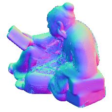

form an irradiance matrix Ei for the hypothesized surface -
 Ω ⊂ ℝ,
normal ni . Using Bi and Ei instead of B and E, Eq. (2) ran( #)
 ran( $)

 #
becomes

 $
 m ' Ei Bi c =
 def
 Di c, 
 $ #
 0
where Di (= Ei Bi ) ∈ RL ×M . For the overdetermined
case L0 > M , the least-squares solution for the BRDF co- Figure 3: Geometric interpretation of the reconstruction er-
efficients c that best explains the measurements, is 2
 ror. The reconstruction error of measurements kZi mk2 can
 
−1 > be seen as distance between the measurement vector m and
 c∗ = D > D D m = D†i m, the subspace spanned by Di in the L0 -dimensional space Ω.

where D†i is Di ’s pseudo-inverse. The estimated BRDF co-
efficients c∗ are least-squares optimal for the hypothesized As illustrated in Fig. 3, a measurement vector m ex-
normal ni and the space of sampled BRDFs Bi . We can ists in an L0 -dimensional space Ω. The column vectors
test the validity of the hypothesized ni by evaluating the `2 of Di span a rank(Di )-dimensional subspace in Ω, and
reconstruction error as the measurement reconstructions Di c∗ = Di D†i m reside
 2
 in this subspace. Thus, geometrically, the reconstruction
 ei = km − Di c∗ k2 . (3) 2
 error kZi mk2 can be considered as the distance between
 the measurement vector m and the subspace spanned by
Therefore, the optimal surface normal n∗ can be found as Di . From this perspective, if rank(Di ) = L0 , the columns
the minimizer of the following objective of Di span the entire Ω; therefore, the reconstruction error
 becomes always zero regardless of the correctness of the
 n∗ = ni∗ , i∗ = argmin ei . (4)
 i∈{1,...,N } hypothesized surface normal n.
 To avoid such a situation, we reduce the column dimen-
A naı̈ve implementation may require a significant computa- sion of Di from M to M 0 < L0 if L0 < M . Specifically,
tion effort for solving this problem. We therefore introduce we apply singular value decomposition (SVD) to Di as
an efficient precomputation strategy now.
 Di = USV> ,
4.2. Precomputation
 and reduce the dimensionality of Di using the first M 0 sin-
 The reconstruction error ei for the hypothesized surface
 gular vectors / values as
normal ni in Eq. (3) can be further simplified as
 >
 2 Di ← UM 0 SM 0 VM 0,

 Di D†i m
 2
 ei = km − Di c∗ k2
 = m−
 >
 2 where UM 0 , SM 0 , and VM 0 are the truncated singular vec-
   2
 = I − Di D†i m = def 2
 kZi mk2 , (5) tors / values.
 2 We empirically found that the proper value of M 0 is re-
 0 0 lated to the noise level in the observations. In Sec. 5.4,
where Zi (= I − Di D†i ) ∈ RL ×L is uniquely determined we examine the accuracy of surface normal estimation with
given a hypothesized normal ni . We can precompute a set varying M 0 and discuss the choices for M 0 .
of {Zi } for all normal candidates in N and at test time we
simply need to assess the magnitude of Zi m for all i. 5. Experiments
 This precomputation happens only once and the result
can be used for any new scene as long as the light configu- This section describes the results of experiments with
ration is unchanged. synthetic and real-world data. We further discuss the com-
 putation time, the effect of dimensionality reduction and the
4.3. Dimensionality reduction of Di discretization of the space of light directions. We begin with
 In principle, minimizing Eq. (4) gives us a correct so- describing the construction of the BRDF tensor and the syn-
lution for the surface normal n. In practice, however, we thetic and real-world datasets that we use for evaluation.
need to pay attention to the dimension and range of matrix
 0
Di ∈ RL ×M . Specifically, when L0 < M or m ∈ ran(Di ) BRDF tensor: The BRDF tensor is constructed from
(the range of Di ) for all Di , there exists one or more BRDF three components; materials, surface normal candidates,
coefficient vectors c∗ that makes all reconstruction errors and light directions. As materials, we used the MERL
{ei } zero. BRDF dataset [16] which consists of 100 distinct BRDFs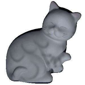

25
 Model-based
error (degrees)
 Mean angular

 20 CNN-based
 15 Ours
 10
 5
 0
 violet-rubber
 light-red-paint
 blue-rubber

 specular-blue-phenolic

 specular-violet-phenolic

 black-oxidized-steel
 dark-red-paint
 orange-paint
 pure-rubber
 yellow-paint
 gold-paint
 yellow-plastic
 pink-felt

 silver-metallic-paint2
 pink-fabric
 neoprene-rubber
 teflon
 red-plastic

 silicon-nitrade

 grease-covered-steel
 pvc
 pink-plastic
 delrin
 gray-plastic
 violet-acrylic
 silver-paint
 white-diffuse-bball
 polyethylene
 white-paint
 green-plastic
 pearl-paint
 cherry-235
 white-acrylic
 specular-white-phenolic

 red-specular-plastic
 colonial-maple-223
 alumina-oxide
 green-metallic-paint
 fruitwood-241
 specular-maroon-phenolic
 gold-metallic-paint3
 purple-paint
 specular-green-phenolic
 pink-jasper
 green-acrylic
 yellow-matte-plastic
 red-fabric2
 nylon
 red-phenolic
 dark-specular-fabric
 ipswich-pine-221
 two-layer-gold
 polyurethane-foam
 beige-fabric
 specular-red-phenolic
 pickled-oak-260
 maroon-plastic
 natural-209
 aventurnine
 white-fabric
 white-marble
 blue-acrylic
 specular-orange-phenolic
 two-layer-silver
 red-metallic-paint
 gold-metallic-paint2
 specular-yellow-phenolic
 blue-fabric
 green-fabric
 hematite

 blue-metallic-paint2
 alum-bronze
 black-soft-plastic
 dark-blue-paint
 yellow-phenolic
 green-metallic-paint2
 black-obsidian
 red-fabric
 specular-black-phenolic
 color-changing-paint2
 white-fabric2
 nickel
 color-changing-paint3
 silver-metallic-paint
 gold-metallic-paint
 pink-fabric2
 light-brown-fabric
 blue-metallic-paint
 green-latex
 chrome
 black-phenolic
 ss440
 special-walnut-224
 color-changing-paint1
 brass
 black-fabric
 chrome-steel
 tungsten-carbide
 steel
 aluminium
 Materials
 Figure 4: Evaluation on the MERL sphere dataset. We compared our method against a model-based method [13] and a
 CNN-based method [12]. The average/variance of the mean angular errors over all materials are as follows: Ours: 2.23/3.24,
 model-based method [13]: 4.31/29.43, CNN-based method [12]: 3.15/9.19.

 including diffuse, specular, and metallic materials. For 5.1. Evaluation on synthetic data
 surface normal candidate sampling we followed Hui’s
 method [11] and obtained 20001 candidates by 0.5◦ equian- We performed experiments on synthetic data to confirm
 gular sampling over the hemisphere [8]. In all experiments that our method works with diverse materials. Since there
 of this paper, we assume that the BRDF tensor contains the is no global illumination in the MERL sphere & bunny
 known light directions. dataset, we can evaluate only the ability of our method to
 adapt to diverse materials. To support that our method is
 applicable to a more diverse set of materials than exist-
 MERL sphere: We created a MERL sphere dataset, ing methods, we compared it against a model-based [13], a
 which is synthetic data rendered with 100 isotropic BRDFs CNN-based [12], and a dictionary-based method [11]. Ad-
 from the MERL BRDF database [16]. We generated im- ditionally, we investigated the accuracy of our method with
 ages of a sphere object illuminated from 20, 40, 60, 80, 100 varying surface normal candidates and lights, and compared
 different known directions1 , respectively. We also created a it to the dictionary-based method [11]. All following exper-
 noisy MERL sphere dataset by adding signal-independent iments were performed in the 80 lights setting unless other-
 and signal-dependent noise [17] to the MERL √ sphere wise specified.
 dataset. The noise model is m̃ = m + (µ + λ m)X where
 m̃ and m are image signals with and without noise, µ
 and λ are weighting factors for signal-independent and
 signal-dependent noise, respectively, and X is a N (0, 1)- MERL sphere: We performed a comparative experiment
 distributed random variable. between our method, the model-based method [13], and the
 CNN-based method [12], and verified that our method is
 more accurate and stable on diverse material data. For the
 MERL bunny: We rendered the Stanford bunny with materials we used a leave-one-out scheme, testing it on one
 spatially varying materials using 11 distinct MERL BRDFs MERL BRDF while constructing the BRDF tensor from the
 as test BRDFs and 80 different known light directions. remaining 99 BRDFs.2
 The results are shown in Fig. 4. The average/variance of
 the mean angular errors over all materials are 2.23/3.24 for
 Real-world benchmark: We took an existing real-world
 our method, 4.31/29.43 for the model-based method [13],
 dataset, the DiLiGenT dataset [20], which contains 10 real
 and 3.15/9.19 for the CNN-based method [12]. This result
 objects of general reflectance illuminated from 96 differ-
 suggests that our method is more accurate and stable than
 ent known directions. This dataset provides ground truth
 existing methods on most materials in the MERL database.
 surface normal maps for all objects measured by high-
 precision laser scanning, enabling quantitative evaluation.
 2 Due to the high computational costs of the dictionary-based
 1 We
 used the generalized spiral points algorithm for uniformly dis- method [11], a leave-one-out scheme on it with the author’s implemen-
 tributing lights on the hemisphere [18]. See the supplementary material tation cannot be performed in a reasonable amount of time. We do a com-
 for details of the light distributions. parison with it in the following experiments.

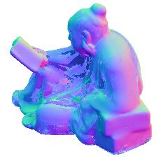
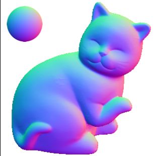
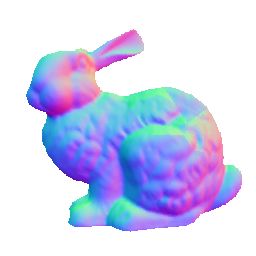
20°+

 10°

 0°

 1.36/2.24 2.16/4.07 4.98/36.13 1.37/2.39
 Ground truth & Dictionary-based [11]
 Ours CNN-based [12] Model-based [13]
 observation
Figure 5: Visual comparison for the Stanford bunny with spatially varying materials. We show estimated normals and angular
error maps of our and 3 comparison methods. Values under the error maps indicate the mean/variance of angular errors.

MERL bunny: We evaluated our method, the model- Table 1: Mean angular errors for estimated surface normals
based [13], the CNN-based [12], and the dictionary-based in degrees for varying numbers of normal candidates.
method [11] on the Stanford bunny with spatially vary-
 number of normal candidates N
ing materials. Our BRDF tensor and the BRDF dictio- 20001 10001 1501 251
nary of the dictionary-based method are constructed from
80 MERL BRDFs that do not include the 11 test BRDFs Ours 2.25 2.31 2.86 4.62
mentioned above. HS17 [11] 2.34 2.41 3.00 4.68
 In Fig. 5 we show each method’s estimated surface nor-
 Table 2: Mean angular errors for estimated surface normals
mals and angular error map. The values under the error
 in degrees for varying numbers of lights.
maps indicate the mean/variance of their angular errors.
This result suggests that our method can be applied to ma- number of lights L0
terials that are difficult for the CNN-based and the model- 100 80 60 40 20
based method. Additionally, from the low variance of an- Ours 2.22 2.25 2.28 2.35 2.69
gular errors we can see that our method is more stable than HS17 [11] 2.30 2.34 2.39 2.49 2.81
the existing methods on diverse materials.

 Tables 1 and 2 show the experimental results for vary-
Varying number of surface normal candidates and
 ing numbers of surface normal candidates and lights, re-
lights: We investigate the angular errors of the estimated
 spectively. Both results suggest that our method consis-
surface normals for varying numbers of surface normal
 tently estimates surface normals more accurately than the
candidates and lights, and compare our method to the ex-
 existing method. One of the reasons is a difference in the
isting search-based method [11]. In the experiment with
 search strategies. Hui and Sankaranarayanan [11] proposed
a varying number of surface normal candidates, we use
 a search strategy that avoids searching parts of the surface
20001, 10001, 1501, 251 surface normal candidates yielded
 normal space since their method is computationally expen-
by 0.5◦ , 1◦ , 3◦ , 5◦ equiangular sampling, respectively. In
 sive due to iterative optimization. In contrast, our method
the experiment with a varying number of lights, we use the
 searches over all surface normal candidates in reasonable
MERL sphere dataset with 20, 40, 60, 80, 100 lights. Due
 computation time facilitated by the precomputation.
to the high computational costs of the existing dictionary-
based method [11], we perform a 5-fold cross-validation,
 5.2. Evaluation on real-world data
using 80 BRDFs for computing our method’s BRDF tensor
and the dictionary method’s material dictionary [11], and We show quantitative comparisons on the DiLiGenT
testing on the MERL sphere dataset with the remaining 20 dataset in Tab. 3 where we compare our method with ex-
BRDFs. isting methods in terms of mean angular error. Here, our

Table 3: Comparisons on the DiLiGenT dataset. We apply a least-squares method as baseline. The values represent mean
angular error (MAE).

 Ball Bear Buddha Cat Cow Goblet Harvest Pot1 Pot2 Reading Avg.

 Ours 1.58 6.38 13.69 6.30 7.80 11.42 18.74 6.67 7.26 15.49 9.53

 SI18 [12] 2.20 4.10 7.90 4.60 7.90 7.30 13.90 5.40 6.00 12.60 7.20
 HS18 [11] 1.33 5.58 8.48 4.88 8.23 7.57 15.80 5.16 6.41 12.08 7.55
 CH18 [3] 2.80 7.60 7.90 6.20 7.30 8.60 15.90 7.10 7.30 13.30 8.40
 TM18 [22] 1.47 5.79 10.36 5.44 6.32 11.47 22.59 6.09 7.76 11.03 8.83
 ST14 [21] 1.74 6.12 10.60 6.21 13.90 10.10 25.40 6.51 8.78 13.60 10.30
 IA14 [13] 3.34 7.11 10.50 6.74 13.10 9.71 26.00 6.64 8.77 14.20 10.60
 Baseline 4.10 8.39 14.90 8.41 25.60 18.50 30.60 8.89 14.70 19.80 15.40

 20°+
Cat

 10°

 0°
Reading

 Observation Ground truth Ours CNN-based [12]
Figure 6: Visual comparison for the non-convex objects Cat and Reading. We show estimated normals and angular error
maps of our method and a state-of-the-art CNN-based method [12].

method does not achieve the best results. This is considered Table 4: Computation time in seconds for surface normal
to be due to factors not modeled in our method, namely estimation of one pixel with 20001 surface normal candi-
cast shadows or inter-reflections. Figure 6 shows visual dates, measured on one core of an Intel Xeon CPU E5-2680
comparisons between our method and Ikehata’s CNN-based v4 @ 2.40GHz.
method [12] for two non-convex objects with cast shad-
 number of lights L0
ows and inter-reflections. Our method causes a large an- 100 80 60 40 20
gular error in pixels where cast shadows or inter-reflections
are likely to occur. However, in convex parts our method Time [sec.] 0.31 0.21 0.15 0.062 0.024
outperforms the CNN-based state-of-the-art method and es-
timates the surface normals well for the Reading object’s
complex specular material. We show more visual compar- the computation time per pixel for 20001 surface normal
isons in the supplementary material. candidates and a varying number of lights L0 . The compu-
 tation is highly parallelizable, e.g., by pixel-wise or normal
5.3. Computation cost candidate-wise parallelization.

 For inference, our method evaluates the reconstruction 5.4. Choice of dimension M 0 for noisy data
 2
error kZi mk2 in Eq. (5) for each surface normal candidate
ni ∈ N . All matrices Zi are precomputed; therefore, at It is difficult to avoid imaging noise in real-world data
inference time we only need to evaluate the reconstruction and it must therefore always be considered. We empirically
error of each ni and find the minimizer. The dimension of observed that M 0 is related to our method’s robustness to-
 0 0
matrix Zi ∈ RL ×L only depends on the number of lights wards noise. Thus, we determine an optimal M 0 by a vali-
 0
L , but not the number of materials. Table 4 summarizes dation on the noisy MERL sphere dataset.

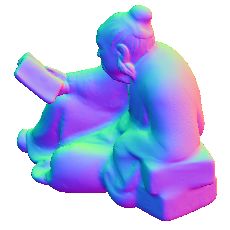
Table 5: Surface normal estimation with varying M 0 on the noisy MERL sphere dataset under three sets of lights, (a) 60 lights,
(b) 80 lights, and (c) DiLiGenT’s 96 lights. Values indicate mean angular errors in degrees.
 (a) (b) (c)
 µ/λ µ/λ µ/λ
 M0 0/0 5/30 30/5 30/30 M0 0/0 5/30 30/5 30/30 M0 0/0 5/30 30/5 30/30
 3 2.21 3.99 3.65 4.37 3 2.18 3.99 3.83 4.43 3 2.59 5.60 5.15 6.22
 5 1.83 4.10 3.52 4.50 5 1.76 4.12 3.71 4.57 5 2.38 6.19 5.20 6.75
 10 1.71 4.29 3.53 4.71 10 1.62 4.30 3.72 4.77 10 2.33 7.08 5.39 7.62
 20 1.75 4.95 3.84 5.33 20 1.62 4.68 3.88 5.12 20 2.37 8.07 5.70 8.65

Setup: We apply 5-fold cross-validation on the MERL Table 6: The effect of discretizing the light directions and
BRDFs; the 100 MERL BRDFs are divided into 80 picking the directions closest to a set of known directions.
BRDFs for the BRDF tensor and 20 BRDFs for test- The values indicate mean angular error in degrees.
ing. We test varying M 0 = {3, 5, 10, 20} and varying noise
 number of lights L0
µ/λ = {0/0, 5/30, 30/5, 30/30} under three sets of lights: 100 80 60 40 20
60 lights, 80 lights, and DiLiGenT’s 96 lights.
 Using known lights 2.15 2.18 2.21 2.31 2.69
 Using discretized lights 2.16 2.19 2.22 2.33 2.73
Results: Table 5 shows mean angular errors of estimated
surface normals in degrees for varying M 0 . In the noiseless
cases (µ = λ = 0), a larger M 0 performs better. Contrarily, with known light directions each time one works with a new
in most of the noisy cases, M 0 = 3 produces lower angular light setup.
errors, indicating that M 0 = 3 is most robust to noise. For
this reason, we apply M 0 = 3 in all following experiments. 6. Discussion
5.5. Discretized light directions In this paper, we have presented a photometric stereo
 In all experiments so far, we assumed that the BRDF method based on discrete hypothesis-and-test search. The
tensor contains the known light directions. In practice, the proposed method can work with a diverse set of BRDFs that
BRDF tensor rarely contains all of the known light direc- are represented in a BRDF tensor and can determine surface
tions and we should use pre-defined light directions closest normals of a scene with spatially varying general BRDFs.
to the known light directions instead. Here, we examine By putting most of the computation into a precomputation
how the surface normal estimation accuracy is affected by step, we enabled a full search over all surface normal candi-
the discretization of light directions. dates, leading to a solution guaranteed to be optimal within
 the bounds of the objective function and the discretization.
 The approach is also supported by the fact that with the con-
Setup: As pre-defined light directions in the BRDF tensor
 tinuing increase of computation power, memory size, and
we used 20001 discretized directions from a 0.5◦ equiangu-
 the availability of many-core processors, the applicability
lar sampling over the hemisphere. When a set of known
 of the full search strategy is expanding. We are interested in
light directions is given, as illustrated in Fig. 2, we can slice
 seeing more applications along the direction.
out a sampled BRDF matrix for a hypothesized surface nor-
 One interesting question to investigate in the future
mal and the set of light directions that are closest to the
 would be how many BRDFs are needed to fully represent
known light direction in terms of cosine distance. We can
 real-world materials. Our BRDF tensor can hold an arbi-
then follow the same estimation process used so far. We
 trary number of BRDFs; therefore, we are interested in in-
performed this experiments with 20, 40, 60, 80, 100 known
 creasing the number of BRDFs in the tensor to study this
lights. We used the MERL sphere dataset and performed
 question, while it may only be empirically understood.
5-fold cross-validation over the BRDFs.
 Acknowledgements
Results: Table 6 shows surface normal estimation results
for exactly known and for discretized light directions in the This work was supported by JSPS KAKENHI Grant
BRDF tensor. We observe that there are only slight dif- Number JP19H01123. Michael Waechter was supported
ferences between both cases (< 0.1◦ in the mean angular through a postdoctoral fellowship by the Japan Society for
errors), which suggests that it is sufficient to precompute a the Promotion of Science (JP17F17350). Kiriakos N. Kutu-
BRDF tensor for sufficiently finely discretized light direc- lakos was supported by the Natural Sciences and Engineer-
tions and there is no need to recalculate the BRDF tensor ing Research Council of Canada under the RGPIN program.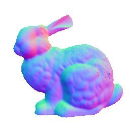

References [16] Wojciech Matusik, Hanspeter Pfister, Matt Brand, and
 Leonard McMillan. A data-driven reflectance model. Trans-
 [1] Neil Alldrin, Todd Zickler, and David Kriegman. Pho- actions on Graphics (TOG), 22(3):759–769, 2003. 2, 4, 5
 tometric stereo with non-parametric and spatially-varying [17] Netanel Ratner and Yoav Y. Schechner. Illumination multi-
 reflectance. In Computer Vision and Pattern Recognition plexing within fundamental limits. In Computer Vision and
 (CVPR), 2008. 1 Pattern Recognition (CVPR), 2007. 5
 [2] Brent Burley. Physically-based shading at Disney. In SIG- [18] Edward B. Saff and Arno Kuijlaars. Distributing many points
 GRAPH, 2012. 2 on a sphere. The Mathematical Intelligencer, 19(1):5–11,
 [3] Guanying Chen, Kai Han, and Kwan-Yee Kenneth Wong. 1997. 5
 PS-FCN: A flexible learning framework for photometric [19] Hiroaki Santo, Masaki Samejima, Yusuke Sugano, Boxin
 stereo. In European Conference on Computer Vision Shi, and Yasuyuki Matsushita. Deep photometric stereo net-
 (ECCV), 2018. 2, 7 work. In Workshops of the International Conference on Com-
 [4] Lixiong Chen, Yinqiang Zheng, Boxin Shi, Art Subpa-Asa, puter Vision (ICCVW), 2017. 2
 and Imari Sato. A microfacet-based reflectance model for [20] Boxin Shi, Zhipeng Mo, Zhe Wu, Dinglong Duan, Sai-Kit
 photometric stereo with highly specular surfaces. In Com- Yeung, and Ping Tan. A benchmark dataset and evaluation
 puter Vision and Pattern Recognition (CVPR), 2017. 1, 2 for non-Lambertian and uncalibrated photometric stereo.
 [5] Tongbo Chen, Michael Goesele, and Hans-Peter Seidel. Transactions on Pattern Analysis and Machine Intelligence
 Mesostructure from specularity. In Computer Vision and Pat- (PAMI), 41(2):271–284, 2019. 5
 tern Recognition (CVPR), 2006. 2 [21] Boxin Shi, Ping Tan, Yasuyuki Matsushita, and Katsushi
 [6] Hin-Shun Chung and Jiaya Jia. Efficient photometric stereo Ikeuchi. Bi-polynomial modeling of low-frequency re-
 on glossy surfaces with wide specular lobes. In Computer flectances. Transactions on Pattern Analysis and Machine
 Vision and Pattern Recognition (CVPR), 2008. 2 Intelligence (PAMI), 36(6):1078–1091, 2014. 1, 2, 7
 [7] Athinodoros S. Georghiades. Incorporating the Torrance [22] Tatsunori Taniai and Takanori Maehara. Neural inverse ren-
 and Sparrow model of reflectance in uncalibrated photomet- dering for general reflectance photometric stereo. In Inter-
 ric stereo. In International Conference on Computer Vision national Conference on Machine Learning (ICML), 2018. 7
 (ICCV), 2003. 2 [23] Silvia Tozza, Roberto Mecca, Marti Duocastella, and Alessio
 Del Bue. Direct differential photometric stereo shape recov-
 [8] Radoslav Harman and Vladimı́r Lacko. On decompositional
 ery of diffuse and specular surfaces. Journal of Mathemati-
 algorithms for uniform sampling from n-spheres and n-balls.
 cal Imaging and Vision, 56(1):57–76, 2016. 2
 Journal of Multivariate Analysis, 101(10):2297–2304, 2010.
 5 [24] Olivia Wiles and Andrew Zisserman. SilNet: Single-
 and multi-view reconstruction by learning from silhouettes.
 [9] Aaron Hertzmann and Steven M. Seitz. Example-based pho-
 British Machine Vision Conference (BMVC), 2017. 2
 tometric stereo: Shape reconstruction with general, varying
 [25] Robert J. Woodham. Photometric method for determining
 BRDFs. Transactions on Pattern Analysis and Machine In-
 surface orientation from multiple images. Optical Engineer-
 telligence (PAMI), 27(8):1254–1264, 2005. 1, 2, 3
 ing, 19(1):139–144, 1980. 1, 2
[10] Berthold KP Horn and Katsushi Ikeuchi. The mechanical
 [26] Sai-Kit Yeung, Tai-Pang Wu, Chi-Keung Tang, Tony F.
 manipulation of randomly oriented parts. Scientific Ameri-
 Chan, and Stanley J. Osher. Normal estimation of a transpar-
 can, 251(2):100–113, 1984. 2
 ent object using a video. Transactions on Pattern Analysis
[11] Zhuo Hui and Aswin C. Sankaranarayanan. Shape and and Machine Intelligence (PAMI), 37(4):890–897, 2014. 2
 spatially-varying reflectance estimation from virtual exem-
 plars. Transactions on Pattern Analysis and Machine Intelli-
 gence (PAMI), 39(10):2060–2073, 2017. 1, 2, 3, 5, 6, 7
[12] Satoshi Ikehata. CNN-PS: CNN-based photometric stereo
 for general non-convex surfaces. In European Conference
 on Computer Vision (ECCV), 2018. 2, 5, 6, 7
[13] Satoshi Ikehata and Kiyoharu Aizawa. Photometric stereo
 using constrained bivariate regression for general isotropic
 surfaces. In Computer Vision and Pattern Recognition
 (CVPR), 2014. 1, 2, 5, 6, 7
[14] Micah K. Johnson and Edward H. Adelson. Shape estima-
 tion in natural illumination. In Computer Vision and Pattern
 Recognition (CVPR), 2011. 2
[15] Feng Lu, Xiaowu Chen, Imari Sato, and Yoichi Sato.
 SymPS: BRDF symmetry guided photometric stereo for
 shape and light source estimation. Transactions on Pattern
 Analysis and Machine Intelligence (PAMI), 40(1):221–234,
 2018. 1