Spatio-temporal Variation of Bright Ephemeral Features on Titan's North Pole - IOPscience
←
→
Page content transcription
If your browser does not render page correctly, please read the page content below
The Planetary Science Journal, 1:31 (11pp), 2020 September                                                                      https://doi.org/10.3847/PSJ/ab9c2b
© 2020. The Author(s). Published by the American Astronomical Society.

         Spatio-temporal Variation of Bright Ephemeral Features on Titan’s North Pole
    Rajani D. Dhingra1,2 , Jason W. Barnes2 , Michael F. Heslar2, Robert H. Brown3, Bonnie J. Buratti1, Christophe Sotin1,
        Jason M. Soderblom4 , Sebastien Rodriguez5, Stéphane Le Mouélic6 , Philip D. Nicholson7, Kevin H. Baines8,
                                           Roger N. Clark9, and Ralf Jaumann10
                               1
                                   Jet Propulsion Laboratory, Caltech, Pasadena, CA, USA; rhapsodyraj@gmail.com, rajani.dhingra@jpl.nasa.gov
                                                           2
                                                              Department of Physics, University of Idaho, Moscow, ID, USA
                                                    3
                                                      Department of Planetary Sciences, University of Arizona, Tucson, AZ, USA
                                               4
                                                 Department of Earth, Atmospheric and Planetary Sciences, MIT, Cambridge, MA, USA
                                              5
                                                Université de Paris, Institut de physique du globe de Paris, CNRS, F-75005 Paris, France
                                          6
                                            Laboratoire de Planetologie et Geodynamique, CNRS UMR6112, Universite de Nantes, France
                                                             7
                                                               Cornell University, Astronomy Department, Ithaca, NY, USA
                                            8
                                              Space Science & Engineering Center, University of Wisconsin-Madison, Madison, WI, USA
                                                                 9
                                                                   Planetary Science Institute, Tucson, AZ 85719, USA
                                                          10
                                                             Deutsches Zentrum für Luft- und Raumfahrt, D-12489, Germany
                                         Received 2019 December 9; revised 2020 June 1; accepted 2020 June 2; published 2020 July 28

                                                                    Abstract
             We identify and document the instances of bright ephemeral features (BEF)—bright areas that appear, disappear,
             and shift from flyby to flyby on Titan’s north pole, using the Cassini Visual and Infrared Mapping Spectrometer
             data set, thereby developing a sense of their spatial distribution and temporal frequency. We find that BEFs have
             differing geographic location and spatial extents. However, they have similar observation geometries and orders of
             surface area coverage and are mostly accompanied by specular reflections. We find the BEFs to represent either
             broad specular reflection off of a recently wetted surface on the north pole of Titan or a near-surface fog—both
             owing to probable recent rainfalls. Our surface model constrains the surface roughness to be of 9°–15° indicating
             the approximate vertical relief of the region to be that of cobbles. We also find that within less than two Titan days
             the BEF (if on the surface) might infiltrate into the subsurface. We hypothesize the parts of BEFs that extend into
             the maria to be precipitation fog.
             Unified Astronomy Thesaurus concepts: Saturnian satellites (1427)

                                     1. Introduction                                      at the south pole, when Cassini arrived during southern summer,
                                                                                          and then later in the equatorial region. These observations were
   Detection of surface changes on Titan have been difficult
                                                                                          broadly consistent with the global circulation models (Tokano &
owing to its complex and thick atmosphere (Kuiper 1944). The
                                                                                          Neubauer 2005; Rannou et al. 2006; Mitchell et al. 2006;
absorption and scattering by atmospheric gases and aerosols
                                                                                          Tokano 2011; Lora & Mitchell 2015; Mitchell & Lora 2016).
(Tomasko & Smith 1982) and the non-Lambertian surface
                                                                                          The circulation models also predicted increasing cloud and rain
phase functions (Solomonidou et al. 2014) make it difficult to
                                                                                          activity at the north pole as north polar summer approached.
hash out the surface signal from that of the atmosphere.
                                                                                             VIMS and ISS finally observed the onset of cloud activity on
Definitive surface changes could be credited to rainfall events
                                                                                          the north pole of Titan (Turtle et al. 2018). Moreover VIMS
on Titan’s surface but have been observed otherwise too
                                                                                          also observed bright ephemeral features (BEFs) on the north
(MacKenzie et al. 2019; Heslar et al. 2020). Of the rainfall
                                                                                          pole of Titan in the T120 flyby (2016 June 7). Dhingra et al.
events documented, one happens to be at the south pole of
                                                                                          (2019) attribute the observation in the T120 flyby to broad
Titan over the Arrakis Planitia (Turtle et al. 2009). Another
                                                                                          specular reflection off of a wetted land surface. When a rough
detected surface change later attributed to giant cloudbursts was
                                                                                          surface gets wetted by rainfall, liquid methane drapes over the
found at the equatorial region (Turtle et al. 2011; Barnes et al.
                                                                                          crests and troughs forming a thin surface layer (Figure 1). This
2013a). Both of these observations were detected by Imaging
                                                                                          liquid layer smooths out the surface at small scales that are
Science Subsystem (ISS) but the equatorial observation was
                                                                                          comparable to the VIMS wavelengths (1–5 μm) and hence are
later followed by Visual and Infrared Mapping Spectrometer
                                                                                          observed as a broadly specularly reflecting layer that is away
(VIMS) as well. Dhingra et al. (2019) discuss the surface
                                                                                          from the specular point. When viewed far from a specular
changes observed over Titan’s north pole hypothesized as
either a wet sidewalk (WSW) feature indicating a recently                                 geometry, a wet surface would appear darker than a dry surface
rainfall wetted surface that reflects brightly at 5 μm or on a                             (Figure 1), as seen by ISS in previous wetting events (Turtle
near-surface fog.                                                                         et al. 2009, 2011). But when viewed somewhat near a specular
   Cloud coverage (Griffith et al. 2009; Rodriguez et al. 2009,                            observation geometry, the area would reflect brightly.
2011; Turtle et al. 2009, 2011, 2018; Brown et al. 2010;                                     Motivated by the T120 observation (Dhingra et al. 2019), we
le Mouélic et al. 2018) and surface rain were both first observed                          sift through other VIMS north polar observations to detect
                                                                                          more transient features. We find additional transient features—
                                                                                          bright areas that appear, disappear, and shift from flyby to flyby
                 Original content from this work may be used under the terms
                 of the Creative Commons Attribution 4.0 licence. Any further             (Figure 2). In this study, we document the temporal and spatial
distribution of this work must maintain attribution to the author(s) and the title        evolution of these bright areas that we termed BEFs in our
of the work, journal citation and DOI.                                                    discovery paper.

                                                                                      1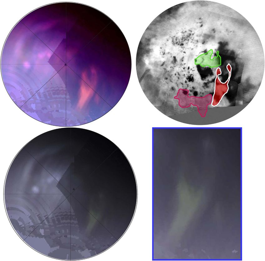
The Planetary Science Journal, 1:31 (11pp), 2020 September                                                                                             Dhingra et al.

Figure 1. We show (in the left) a cartoon to explain the origin of the BEF. The orange ovals are lakes on Titan while the transparent orangish feature is a recently
wetted region. The blue arrow indicates the geometry for direct specular reflection where incidence and emission angles are equal. The cone shows the light reflected
within a small angle of the perfect reflection. The intensity of the reflection tails off outside of the cone. On right we show a WSW effect on a bright morning after
rainfall at the University of Idaho parking lot. The specular reflection (orange arrow) arises out of the rear windshield of the car. The other regions at the right
geometries are reflecting brightly (yellow arrow) or look darker. The south polar darkening that Turtle et al. (2009) documented would be in a geometry like the darker
region in this WSW picture. The figure’s change contrast in the subsequent images due to the various platforms of the analysis.

Figure 2. We show here orthographic projections of VIMS mosaics from eight different Cassini Titan flybys centered on 23°–40°N, 180°E. The color scheme brings
out specular features in orange and clouds in purple (red is mapped to 5 μm, green to 2 μm, and blue to 2.73 μm). The orange arrows show the specular reflection in
each flyby. The purple arrows show the cloud cover over the north pole of Titan. The BEFs are shown by yellow arrows.

   Only a few rainfall observations have been documented in                           BEF challenging. Moreover the polar regions of Titan, where
the 13 years of the Cassini mission. The low frequency of                             BEF occur, are only illuminated during a fraction of the
Titan’s encounters (∼1 flyby per month), the rapid evaporation                         mission duration.
rate (∼30 m/Titan year, from Mitri et al. 2007), and the fact                            Observation geometry, position of the spacecraft, evapora-
that only a small number of atmospheric windows are able to                           tion rate, and atmospheric scattering augment the difficulty
probe the surface (Sotin et al. 2005) make the observation of a                       of observing rainfalls on Titan. The significance of this

                                                                                  2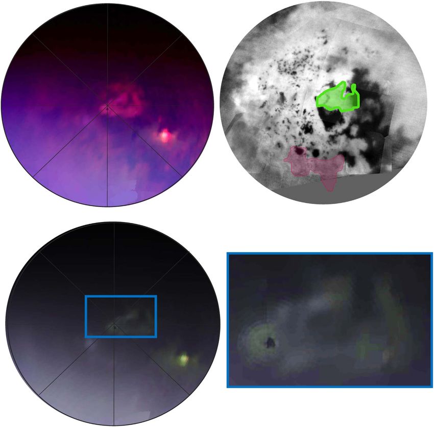
The Planetary Science Journal, 1:31 (11pp), 2020 September Dhingra et al.
Table 1
We Show here Parameters for the VIMS Observations on Various Flybys that Show Indications of the WSW Effect
Flyby Date Phase (deg) Cube Used Exp Time (ms) i (deg) e (deg) Pixel Res (km pixel−1)
T106 2014 Oct 24 120 CM_1792827895_1 160 71 49 37
T119 2016 May 6 125 CM_1841258035_1 160 63 68 24
T120 2016 Jun 7 116 CM_1844022476_1 160 51 64 48
T121 2016 Jul 25 113 CM_1848148220_1 160 63 51 32
T123 2016 Sep 27 112 CM_1853659871_1 180 53 60 38
Note.The best cubes are those acquired near Titan, thereby achieving the finest-scale resolution. The incidence angle (i) and emission angle (e) shown are typical for
the BEF on that particular flyby.
documentation is that we might be able to determine when and the same region covered in previous flybys. The T120 BEF
where has it rained on the north pole of Titan without having to region had been last seen in T106 flyby. While we confirmed
actually observe the rainfall event. that the bright region in T120 was indeed ephemeral owing to
Our study is driven by finding the answer to the question, its absence in T106, we found another BEF in the T106 flyby
“when and where does it rain on Titan?” The answer to which itself. We devised the WSW color composite (Figure 3(a))
will help in the determination of the global methane transport because this helped us in hashing out the clouds in purplish
and global liquid distribution. Cloud observations help us hues, while pinkish features are closer to the surface or near-
determine the probability of rainfall and confirm if local surface. Figure 3(b) shows the ISS map in polar projection and
environmental conditions (e.g., convective and saturated air) the spatial extent of the T120 BEF marked in magenta.
are favorable for rain. However, figuring out the location and Flybys before the T106 do not show any observable BEFs.
time of the rainfall is important to solve the puzzle of the The T106 flyby happened on 2014 October 24 and began the
asymmetric liquid distribution on Titan. series of several directed north polar flybys and BEF
In Section 2, we enlist the data used and the observations of observations. As shown by a yellow arrow in Figure 4(a), the
the BEF in other flybys apart from T120. Section 3 entails each BEF partly covers the land between Punga Mare and Ligeia
observation in detail such that the geographic location and area Mare and extends into Ligeia Mare. The extention into Ligeia
covered. We calculate the surface roughness of the BEFs in Mare is a surprising observation and complicates our analysis
Section 4.1. In Section 4.2, we discuss an approximation of about the BEF’s location vertically, i.e., if it is right on the
the amount of rainfall constrained by evaporation and surface or up in the atmosphere. It is also a possibility that the
infiltration rates. In Section 5, we discuss the possibility of BEF is an amalgamation of two different vertical features—a
BEFs being fog, which is followed by Section 6 with a near surface (over the Mare) and on the surface (WSW)—
discussion, conclusions, and details of future work. seemingly appearing as one feature. The adjacent Figure 4(b)
shows the outline of the extent of the BEF in green. We show
2. Data T120ʼs outline (in magenta) indicating that the BEF’s
We calibrate the Planetary Data System (PDS) data using the geographic location has changed.
algorithm described by Barnes et al. (2007a), except that we The areal coverage of T106 BEF totals ∼115,000 km2 over
turn the despike off. Each cube is despiked by hand as the the latitudes from 90°N to 80°N and longitudes of 210°W to
automated despiker cleans the data of primary specular glints in 300°W. The T106 flyby also has a direct specular reflection on
such a way that degrades its overall utility in a specular context. the eastern edge of Kraken Mare over Gabes Sinus. The
We also use the ISS (https://planetarymaps.usgs.gov/mosaic/ latitude and longitude of the inferred specular point are 70°. 7N,
Titan_ISS_P19658_Mosaic_Global_4km.tif) north polar map 293°W. The great circle distance from the specular point is
to look at the observation in spatial context to manually draw ∼715 km, indicating that the BEF is close enough to the
the contours of the BEF using ArcGIS. specular point (or in the specular cone as shown in Figure 1).
Table 1 documents the data used in this study, the flyby, the We devise a triple peak color composite (R=2.7 μm,
cube used for the analysis, and the observation geometry. We G=2.8 μm, and B=2.9 μm) to better separate the different
basically sift through all the flybys after the T100s (2014 April) portions of a BEF (Figure 4(c)). The 2.7–2.8 μm sub-window
and use the cubes from the flybys where we see a BEF in our (McCord et al. 2006) in Titan spectra looks at the surface. We
WSW color composite (R=5 μm averaged over channels have the longest optical paths through Titan’s atmosphere
336–351, G=2 μm channel 165, and B=2.73 μm channel when we look through an atmospheric window (2.7–2.8 μm
208, Figure 2). in this case; Barnes et al. 2007a, 2007b, 2013b; McCord et al.
2008) and hence have maximum sensitivity to the surface.
3. Details of Each Observation As we move away from the band center and look at the wings
of an atmospheric window, we are looking through more
In addition to the discovery instance of T120 observation,
atmosphere (higher optical depth) while moving away from
we now recognize additional observations that show the BEF
the surface, at some altitude. The wing of the sub-window
on the north pole of Titan. In this section we identify and map
lies at 2.9 μm moving away from the surface. Since we assign
each instance of BEF.
the 2.9 μm window to blue, any whitish feature is probably in
the atmosphere. Similarly we assign the 2.8 μm to green
3.1. T106
so the greenish feature is on the surface or closer to the
Our discovery observation of the BEF in the T120 flyby surface. Motivated by the extensions of BEFs into Titan’s
(Figure 3) happened on 2016 June 7. It motivated us to look for maria, this color composite helps us in ruling out if the other
3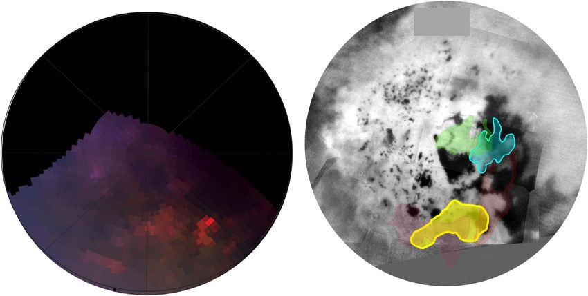
The Planetary Science Journal, 1:31 (11pp), 2020 September Dhingra et al.
Figure 3. Panel (a) shows a polar stereographic projection of T120 flyby in VIMS WSW color composite (red is mapped to 5 μm, green to 2 μm, and blue to
2.73 μm). The orange arrow marks the location of direct specular reflection. Panel (b) shows the extent of T120 WSW marked in magenta over a base map of ISS. The
other magenta feature at the north pole is another WSW feature. The subsequent figures differ in contrast due to the various platforms of analysis.
portions of the BEF are indeed on the surface or at some 3.3. T121
height above the surface. Different parts of the BEF show up T121 (2016 July) is one of the most cloud-heavy flybys of
in different hues of white or green in every flyby based upon the north pole and probably the whole Cassini mission. The
the color scheme. north pole is almost totally under cloud cover in our WSW
The feature at the north pole (near Punga) looks whitish color composite (see Figure 6(a)) except the bright BEF
indicating the atmospheric location of the BEF. The extension peeking through the clouds and the southern Kraken Mare.
of the BEF into Ligeia Mare looks greenish indicating the The T121 flyby also has a specular reflection that arises from
surface location of the feature (Figure 4(d)). the geographical location 83°N and 6°. 4W. The specular
reflection arises from land (southwest of Punga coast). The
fact that the specular reflection arises from land surface close to
3.2. T119 the Punga coastline might indicate that either it is a wetted
T119 (2016 May) was the preceding observation to our surface or a marshy land near the coastline. However, there are
T120 (2016 June) discovery observation. We see a BEF in the several small lakes observed in the ISS observation in the
T119 flyby yet not at the location where T120 BEF (magenta) vicinity of the specular reflection and it is quite likely that
was. The spatial extent covers an area of ∼70,000 km2 over the glint is coming from one of those lakes. The great circle
the approximate latitudes of 81°N–68°N and longitudes of distance of the center of the core of the BEF feature from the
66°E–17°E. The T119 flyby has no specular observation as the specular point is ∼400 km.
The BEF overlays the land between Ligeia Mare, Punga
predicted specular point does not move over liquid bodies.
Mare, and Kraken Mare (Figure 6(b)). There is a finger-like
The T119 BEF observation overlays the land between Jingpo
feature poking into Ligeia Mare that we call the “Ligeia finger”
Lacus and Kraken Mare as shown in Figure 5(a) in the VIMS
in the rest of this work that is different from the Radio Detection
color composite. Figure 5(b) marks the spatial extent of the
and Ranging (Radar) observations of the magic island
BEF in red. Although the core of this feature overlays land (Hofgartner et al. 2016).The Ligeia finger very prominently
surface, a thin portion juts into Kraken Mare. stands out in the orthographic images of the north pole, making
We use the triple peak color scheme on T119 (Figures 5(c) us question if the location of the “Ligeia finger” or all of the BEF
and (d)) and observe that the laminar extension of T119 BEF is indeed on the surface. The feature could as well be a near-
and the portion of the BEF that overlays Jingpo Lacus look surface feature.
different than the core of the feature. The laminar extension of Our triple peak color scheme (R=2.7 μm, G=2.8 μm, and
T119 BEF is not even perceivable in the triple peak color B=2.9 μm) shows the Ligeia finger along with some portion
scheme. This certainly helps the case of the BEF being a wetted of the BEF in a bluish-white hue as compared to the otherwise
surface; the laminar could be a thin cloud/fog that is near greenish hue of the core BEF (Figures 6(c) and (d)). This could
Kraken’s surface, as may also result from a recent rain event. mean that some regions of the BEF, including the “Ligeia
However, the imperceptibility of the laminar extension could finger” extension of the BEF, are probably located at a different
also just be because a fog over a dark sea is harder to see than a height in the atmosphere. This triple peak analysis indicates
fog over a brighter surface. It is also possible that the fog that the height of the Ligeia finger is different from that of the
changes altitude as it move between land and sea and thus BEF. The finger also has a dark gap in a triple peak image,
appears different from orbit. which may suggest that it is distinct from the BEF.
4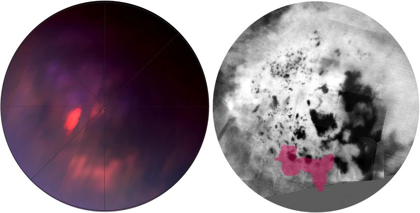
The Planetary Science Journal, 1:31 (11pp), 2020 September Dhingra et al.
Figure 4. Panel (a) shows the polar stereographic projection of T106 flyby in VIMS WSW color composite. The orange arrow marks the location of direct specular
reflection. Panel (b) shows the extent of the T106 BEF in green on the base map of Radar and ISS. Faded magenta outline marks the T120 BEF extent indicating that
the feature is at other geographical locations of the north pole. Panel (c) shows the T106 flyby in the VIMS triple peak color (R=2.69 μm averaged over channels
205–207, G=2.77 μm channels 210–212, and B=2.90 μm channels 218–219) composite. Panel (d) is the zoomed-in and cropped BEF in a triple peak color
scheme. Features at surface look greenish while clouds look whitish blue.
3.4. T123 again indicates an ephemeral puddle, wetted land surface,
marshy shorelines, or a specular glint near the shore of Kraken
The T123 flyby that occurred on 2016 September (the same
just as the waves hit the shoreline. Only a pixel-by-pixel
year as all the other flybys that display BEFs, except T106) is
analysis of all the cube acquired during this flyby can assess the
our last flyby where we see the BEF before the Cassini mission
location and the nature of the specular point.
ended.
However, we can clearly distinguish the BEF in this flyby by
the lower spatial sampling (Figure 7(a)). The BEF overlays the
3.5. Null Detections
land between Jingpo Lacus and Bolsena Lacus and covers an
area of ∼120,000 km2 (Figure 7(b)). A portion of the BEF In between our first BEF detection in the T106 flyby and the
overlays Jingpo Lacus but since this flyby is of a lesser spatial next one in the T119 flyby, there are no north polar Cassini data
sampling we do not run the triple color scheme on this of Titan acquired. The later north polar observations of Titan
observation. Another thing to note is the spatial extent of the (T124, T125, and T126) do show a plethora of cloud cover yet
T123 BEF overlaps that of T120ʼs and T119ʼs partly. The not a BEF. The next flyby, T124, has a specular reflection but
approximate inferred specular point of this flyby is 69°. 56N and no BEF whereas T125 has a probable BEF signature but
33°. 36E that overlays the land surface off the eastern coast of because of very low spatial sampling, we do not include the
southern Kraken Mare. We do observe a direct specular T125 observation in our work here. T126, the final VIMS close
reflection from the land near the shores of Kraken Mare that flyby of Titan, has no detected BEF.
5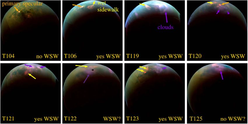
The Planetary Science Journal, 1:31 (11pp), 2020 September Dhingra et al.
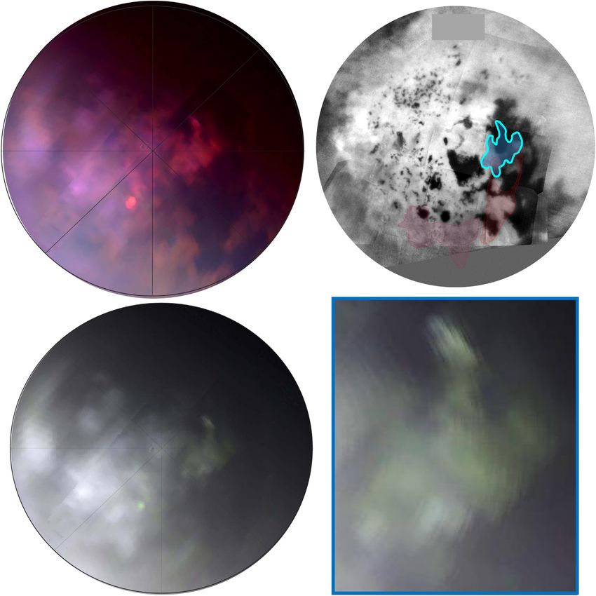
Figure 5. Panel (a) shows the polar stereographic projection of the T119 flyby in VIMS WSW color composite. Panel (b) shows the extent of the T119 BEF in red on
the base map of ISS. Faded magenta and green outlines mark the T120 and T106 BEF extent indicating that the feature is at other geographical locations of the north
pole. Panel (c) shows the T119 flyby in the VIMS triple peak color (R=2.7 μm, G=2.8 μm, and B=2.9 μm) composite. Panel (d) is the zoomed-in and cropped
BEF in a triple peak color scheme. Features at surface look greenish while clouds look whitish blue (see the text for details).
4. WSW Scenario We observe that the surface-roughness values vary between
9° and 15° (Table 2). We use the observational and theoretical
When some of the BEFs are surface features, we can derive
constraints to derive the length scales over which the model-
the surface roughness by using the observation geometry
determined surface roughness occurs.
constraints of a broad specular reflection where the facets are
Surface tension restricts the spread of liquid methane rain
tilted such that the reflection is toward the observer (Cassini).
over an icy bedrock (17 dyne cm−1; Sprow & Prausnitz 1966);
We derive the surface-roughness constraints followed by
water surface tension is 70 dyne cm−1 (Vargaftik et al. 1983).
placing rough restraints on the rainfall volume in the below
Liquid methane spreads readily as it has a lower surface tension
subsections.
than water. Radar data provide an observational constraint,
suggesting the topography of the region to be rough and
variegated at the Radar wavelength scale (∼2 cm). All the
4.1. Surface-roughness Constraints
flybys discussed in this work are on the north pole. We see that
We use a numerical planetary specular model (Soderblom the BEF regions usually overlap the Synthetic Aperture Radar
et al. 2012; Barnes et al. 2014) with Gaussian-distributed (SAR)-bright, dark dissected uplands and darker, lower plains
slopes and azimuthal symmetry for the same observation that usually have a high local slope (Birch et al. 2017).
geometry as our BEF observations to understand the surface To infer the topography of the BEF regions under these
roughness. This analysis also helps in cataloging the (model- constraints, we assume different grain size dimensions,
derived) surface roughnesses for the north pole for the surface- namely gravel (2–64 mm), cobble (64–256 mm), and boulder
roughness values. (200–630 mm) as length scales and calculate the corresponding
6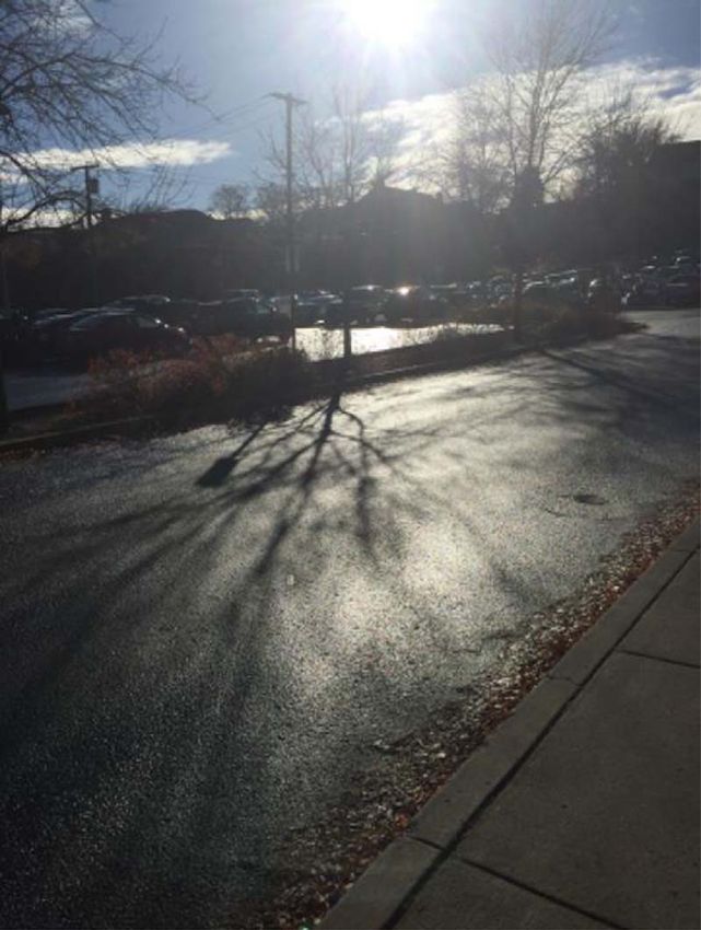
The Planetary Science Journal, 1:31 (11pp), 2020 September                                                                                             Dhingra et al.

Figure 6. Panel (a) shows the polar stereographic projection of the T121 flyby in VIMS WSW color composite. Panel (b) shows the extent of the T121 BEF in cyan
green on the base map of Radar and ISS. Faded magenta, green, and red outlines mark the T120, T106, and T121 BEF extent indicating that the feature is at other
geographical locations of the north pole. Panel (c) shows the T121 flyby in the VIMS triple peak color composite. Ligiea Finger is indicated by a green arrow in the
figure panels (c )and (d). Panel (d) is the zoomed-in and cropped BEF in a triple peak color scheme. Features at surface look greenish while clouds look whitish blue.

vertical relief. If the primary source of our measured ∼9°–15°                                                   4.2. Rain Quantity
surface roughness were gravel, then under the surface-rough-                             We try to place constraints on the quantity of rain delivered
ness conditions, the vertical relief would range from submm to                        to the surface using a simple mass-balance model (Dhingra
a couple of millimeters (0.7–21 mm). If cobbles instead cause                         et al. 2018). Given that the WSWs do not occur in the same
the observed roughness, then the peak to trough surface heights                       place from flyby to flyby, we use their limited longevity along
are ∼21–85 mm. The range (∼8.5 cm) for the values of cobbles                          with models of evaporation (Mitri et al. 2007) and infiltration
is larger than the observational constraint from the Radar data.                      with hydraulic conductivity (Hayes et al. 2008; Horvath et al.
We therefore infer that the geomorphology of the region                               2016) to derive limits on the minimum quantity of liquid that
corresponding to the BEF could be a mix of gravels and small                          could have produced each observed feature.
cobbles of vertical relief ranging from submm to a couple of                             The longevity of the rainfall is derived by the time spans
centimeters that very much sounds like the Huygen’s landing                           between the two flybys. There are no prior observations for
site (Soderblom et al. 2007).                                                         T106 and T119 flybys. However, T120, T121, and T123 flybys

                                                                                 7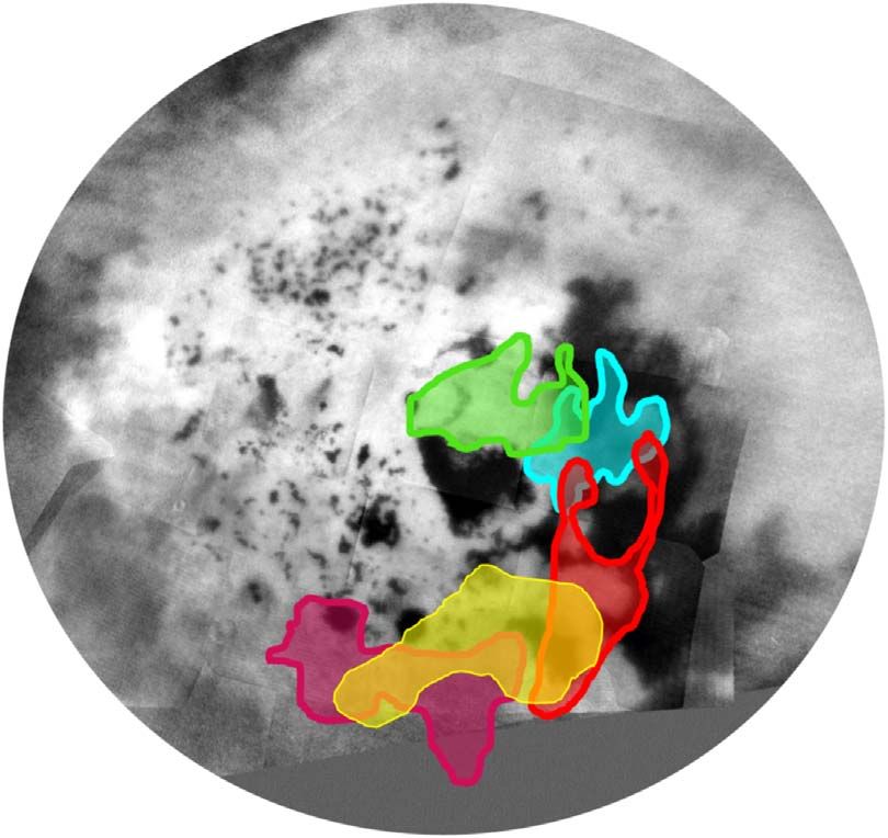
The Planetary Science Journal, 1:31 (11pp), 2020 September Dhingra et al.
Figure 7. Panel (a) shows a polar stereographic projection of T123 flyby in VIMS WSW color composite (red is mapped to 5 μm, green to 2 μm, and blue to
2.73 μm). Panel (b) shows the extent of T123 WSW marked in yellow over a base map of Radar and ISS.
Table 2
We Tabulate the Model-derived Surface-Roughness Values here for Each Flyby BEF Observed
Flyby Cube Used Sp. Pt. Location Dist. from Sp. Pt. (km) Surface Roughness (deg)
T106 CM_1792827895_1 Sea (Kraken) 715 9
T119 CM_1841258035_1 NA NA NA
T120 CM_1844022476_1 Lake (Xolotlan) 632 10–15
T121 CM_1848148220_1 Land (southwest of Punga coast) 424 NA
T123 CM_1853659871_1 Land (Kraken coast) 452 9–10
Note.“NA” in the columns indicate either there was no specular reflection observed to model surface roughness or the model fails to generate a specular reflection that
arises from a land surface.
do have prior flybys to determine their longevities. Table 1 Khy, and the hydraulic conductivity is expressed as
shows that T120 was observed two Titan days after T119
indicating a longevity of maximum two Titan days. Similarly, krg
Khy = . (3 )
T121 was observed three Titan days later, and T123 was m
observed four Titan days later. We use the evaporation rate of
30 m/Titan year (Mitri et al. 2007) and infiltration with Here, κ is the percolation velocity that we use from Horvath
hydraulic conductivity using the percolation velocity of liquid et al. (2016) for low and high permeabilities, ρ is the density of
methane for Titan conditions as assumed in Horvath et al. methane, μ is the viscosity of methane, and g is Titan’s gravity.
(2016). The mass-balance model for this calculation we Our calculations shown in Table 3 indicate that the change in
consider is as given below. Here, V is the volume of the volume of rainfall is a negative quantity for the observed
rainfall, P is the precipitation rate, E is the evaporation rate, Ac longevity if the BEFs behave like a WSW (Figure 1). This
is the catchment area, ABEF is the area of the BEF, and Khy is suggests that if the BEFs are WSW on the surface they must be
the hydraulic conductivity as described in Equation (3): very fresh and less than a few hours old. Rainfall would not be
dV observable after a whole span of two/three/four Titan days and
= (P * A c - (E + Khy) * ABEF ). (1 ) might infiltrate or evaporate before our next observation.
dt
However, we wish to note that this calculation disagrees the
We assume a linear decrease in volume and that Ac=ABEF precipitation induced brightening Barnes et al. (2013a)
(owing to the less solid surface area available on Titan’s north observed in the equatorial region of Titan, where after the
pole): cloudburst the areas darken for months, then brighten for a year
DV = [P * ABEF - (E + Khy) * ABEF ]*Dt, (2 ) before reverting to their original spectrum. In fact, the cold
temperatures near the pole must perhaps freeze the methane
where ΔV is the change in volume, ABEF is the area of the BEF, rain into methane or ethane ice that would melt more slowly
E is the evaporation rate, Δt is the longevity of the BEF and there (Steckloff et al. 2020).
8The Planetary Science Journal, 1:31 (11pp), 2020 September Dhingra et al.
Table 3
We Tabulate the Values We Derive Using Our Mass-balance Model to Approximate the Quantity of Rainfall
Flyby ABEF(∼km 2) Longevity (Titan Days) Change in Volume
T106 115,000 Unknown Unknown
T119 70,273 2 All percolated/evaporated
T120 120,000 3 All percolated/evaporated
T121 120,386 4 All percolated/evaporated
T123 119,340 At least 2 All percolated/evaporated
Note. According to our calculation we would not be able to observe rainfall on Titan’s surface within as less than two Titan days based on (Mitri et al. 2007). A list of
the constants used in table calculations. Precipitation rate=1.2 m/Tyr*. Evaporation rate=30 m/Tyr*. Hydraulic conductivity Khy=3.14 m/Tyr, for high
permeabilities of 1 × 10⁻¹⁴ m2, low permeabilities of 1 × 10⁻¹⁰ m2 ρ, the density of methane=438.9 kg m−3 μ, the viscosity of methane=2×10⁻⁴ Pa/s gravity
of Titan, and g is 1.35 m s−2.
5. Fog Scenario It is conceivable to have a scenario similar to ice crystals in
Earth’s atmosphere observed to produce broad specular
Fogs are clouds in contact with the ground and are formed
reflections and thus appear more orange than purple in the
similarly to clouds—by condensation of warmer air to tiny
BEF color scheme. On Titan, if aerosols (Tomasko et al. 2008)
water droplets. The particle size of fog particles might reflect
formed into little plates and settled in the atmosphere in
brightly as was the case in the discovery of fogs at the south
parallel, we might get a reflection off the oriented plates.
pole of Titan (Brown et al. 2009). Surface heating due to higher
However, even these low-lying, ice-laden clouds should exhibit
summer insolation at the poles might increase the humidity
the high reflectance at 2.7 μm characteristic for clouds (which
especially near the mare or liquid bodies on the north pole. This
is not observed).
methane vapor in the air along with a plethora of available
microscopic solid haze particles raining from the upper
atmosphere might be conducive to form fogs.
The most probable fog candidate that aligns with the BEF 6. Result and Discussion
scenario is “precipitation fog.” As the extra methane vapor (from We report VIMS observations of BEFs over Titan’s north
lakes and puddled rainfall) comes into contact with air that is pole. Their spectral signatures indicate they could be surface to
already heavily saturated after the rainfall, it might cause the air near-surface features. Their proximity to direct specular
to reach the dew point and form fog. However, whether the reflections suggest that these features are broad specular
temperature difference (MacKenzie et al. 2019) between rain reflections. These bright patches lie primarily over land
cloud height and warmer ground would be enough to saturate the surfaces but certain parts of their extend into fluid bodies
air and form precipitation fogs has yet to be formally modeled. highlighting the complex sea–land meteorological conditions at
Other probable scenarios could be “advection fog” or “valley Titan’s sea district (e.g., rain, fog, and convective clouds) as
fog.” Advection fog occurs when warm air moves in over a suggested by previous models (Tokano 2009).
cooler land surface. When warm ocean breezes in over cooler The extension of regions of a BEF into fluid bodies is
land especially along coastlines, the land cools the warm air intriguing. We use a triple peak color scheme to untangle the
below the dew point and advection fog forms. Part of the T106 regions of a BEF extending into liquid bodies. The liquid
feature that aligns with the Ligeia coastline could be advection extensions of T119 and T123 flybys do show up in whitish
fog (Figure 4). hues indicating the non-surficial location of the features.
Valley fog occurs when warm air passes over the upward In the T106 flyby, the extension of a BEF into Ligeia Mare
slope of a cool mountain. As elevation increases, the mountain does not show up in whitish hues. This could either mean that
cools the air quickly, causing condensation and fog. Cook et al. we are looking at wavy liquid surfaces or a near-surface fog/
(2015) classified regions around the Mare in the mountain cloud. A maria with surface roughness of 9°–15° could as well
chain category. Birch et al. (2017) classify regions around the indicate active rainfall. Another possibility is we could just be
north polar maria in their geological map as SAR-bright/dark observing a near-surface cloud that is obstructing the active
dissected terrains, SAR-bright dissected uplands, and moun- rainfall happening at that very instant while Cassini VIMS is
tains. The topographic areas would form fog or low-level looking at the region. We could as well be seeing the falling
orographic clouds in the valleys between mountains or on the drops themselves. The lower gravity and bigger raindrops
windward side of hills. (Lorenz 1993) fall slow compared to Earth and might outlast
If BEFs behave the same as the WSW surface, they would be the cloud sometimes.
expected to occur in flat, open plains with minor changes in Figure 8 shows a time line of the observed BEF features.
surface elevation while fogs are expected in low-elevation Highest precipitation in the warmer colors can be seen a little
valleys between hills/mountains or the leeward side of the before 2015. Our time series suggests that the bright patches
larger seas. According to our color images using the spectro- started in 2014 and picked up by 2016. The northern summer is
scopic windows, if BEF features are fog, they are probably a probably inchoate compared to model predictions but definitely
few km or less off the surface or near-surface fogs. Depending picked up, indicating dynamic progression of the atmosphere–
on the humidity and temperature, fogs can form quickly and surface interaction. The fact that our observations agree with
also disappear very quickly. Such “flash fogs” are transient in the predictions is consistent with the idea that these phenom-
nature. The BEF features could as well be “flash fogs” owing to enon are meteorological. A comparison of Figure 1 of Turtle
their ephemerality. However, their lifetimes can only be et al. (2018) indicates that ISS sees patchy clouds in 2014 and
constrained provided the local climate conditions are known. the cloud activity picks up by 2016 in ISS observations too.
9The Planetary Science Journal, 1:31 (11pp), 2020 September Dhingra et al.
Figure 8. We show all the confirmed BEFs in the above polar plot of Titan. The time line below shows the appearance of the BEF on the north pole. The opaque boxes
show a positive observation of the BEF while the white outlined boxes indicate unconfirmed observation. The numbers preceded by T are the flyby numbers. The
numbers in blue state the month and year the observation was recorded in.
The geographical locations of the BEFs on the north pole are global understanding of methane transport. The knowledge of
intriguing. The BEFs are confined to the polar latitudes north of rainfall patterns might help design flight patterns of Titan aerial
Kraken’s south shoreline (60°N), suggesting that the maria vehicles including balloons (Lorenz 2008a, 2008b; Dorrington
might be driving them. More usually than not the BEFs are 2011; Hall et al. 2011), airplanes (Barnes et al. 2012), and
located near the larger liquids on the north pole. This compels rotorcraft (Turtle et al. 2019).
us to ask if the big seas and the humidity along with solar
heating is driving these BEFs. This may also suggest that much The authors acknowledge support from the NASA/ESA
of the methane humidity must originate from the maria. Cassini Project and the VIMS team. R.D. acknowledges
The solar heating of the north pole results in the warming of the support from NPP (NASA Postdoctoral Program) and the
cooler liquids that increase the humidity content near the Cassini team for all the years of profound work. We thank Dr.
liquid’s surface. This increase in humidity might drive Faith Vilas for coordinating the reviews, Dr. Vincent Chevrier,
rainstorms or rainfall. and an anonymous reviewer for their careful reading and
Titan’s south polar summer deserves to be mentioned in our suggestions that improved our manuscript.
discussion as well. When Cassini arrived in Saturn’s system in
2004 July, the summer had already started in the Southern ORCID iDs
Hemisphere and was in full swing. We did miss the beginning
of the south polar summer. In contrast, we saw the beginning of Rajani D. Dhingra https://orcid.org/0000-0002-3520-7381
the northern polar summer but the Solstice mission ended as Jason W. Barnes https://orcid.org/0000-0002-7755-3530
the northern summer probably was in full swing. Jason M. Soderblom https://orcid.org/0000-0003-
In particular, we saw one large storm in the south polar 3715-6407
summer (Turtle et al. 2011), while cloud activity was frequent Stéphane Le Mouélic https://orcid.org/0000-0001-
(Turtle et al. 2018). In comparison, if the BEFs are rainfall 5260-1367
events or even if they are precipitation fogs, we might have
observed far more events on the north pole of Titan. The References
relative larger liquid cover of the north pole definitely affects
the humidity levels that probably causes the larger cloud cover Barnes, J. W., Brown, R. H., Soderblom, L., et al. 2007a, Icar, 186, 242
Barnes, J. W., Buratti, B. J., Turtle, E. P., et al. 2013a, PlSci, 2, 1
and more dynamic meteorology. Barnes, J. W., Clark, R. N., Sotin, C., et al. 2013b, ApJ, 777, 161
This documentation will help the design and execution of Barnes, J. W., Lemke, L., Foch, R., et al. 2012, ExA, 33, 55
potential future Titan missions. Establishing the WSW effect Barnes, J. W., Radebaugh, J., Brown, R. H., et al. 2007b, JGRE, 112, E11006
technique would permit a future Titan orbiter (Coustenis et al. Barnes, J. W., Sotin, C., Soderblom, J. M., et al. 2014, PlSci, 3, 3
Birch, S. P. D., Hayes, A. G., Dietrich, W. E., et al. 2017, Icar, 282, 214
2009; Mitri et al. 2014; Sotin et al. 2017), or Saturn orbiter with Brown, M. E., Roberts, J. E., & Schaller, E. L. 2010, Icar, 205, 571
multiple Titan flybys, to map surface rainfall using broad Brown, M. E., Smith, A. L., Chen, C., & Ádámkovics, M. 2009, ApJL,
specular reflections. Tighter constraints on rain would improve 706, L110
10The Planetary Science Journal, 1:31 (11pp), 2020 September Dhingra et al.
Cook, C., Barnes, J. W., Kattenhorn, S. A., et al. 2015, JGR, 120, 1220 Mitri, G., Coustenis, A., Fanchini, G., et al. 2014, P&SS, 104, 78
Coustenis, A., Atreya, S., Balint, T., et al. 2009, ExA, 23, 893 Mitri, G., Showman, A. P., Lunine, J. I., & Lorenz, R. D. 2007, Icar, 186,
Dhingra, R. D., Barnes, J. W., Brown, R. H., et al. 2019, GeoRL, 46, 1205 385
Dhingra, R. D., Barnes, J. W., Yanites, B. J., & Kirk, R. L. 2018, Icar, 299, 331 Rannou, P., Montmessin, F., Hourdin, F., & Lebonnois, S. 2006, Sci, 311,
Dorrington, G. E. 2011, AdSpR, 47, 1 201
Griffith, C. A., Penteado, P., Rodriguez, S., et al. 2009, ApJL, 702, L105 Rodriguez, S., le Mouélic, S., Rannou, P., et al. 2009, Natur, 459, 678
Hall, J. L., Lunine, J., Sotin, C., et al. 2011, in Proc. Interplanetary Planetary Rodriguez, S., le Mouélic, S., Rannou, P., et al. 2011, Icar, 216, 89
Probe Workshop 8 (Houston, TX: NASA Johnson Space Center) Soderblom, J. M., Barnes, J. W., Soderblom, L. A., et al. 2012, Icar, 220,
Hayes, A., Aharonson, O., Callahan, P., et al. 2008, GeoRL, 35, L9204 744
Heslar, M. F., Barnes, J. W., Seignovert, B., Dhingra, R. D., & Sotin, C. 2020, Soderblom, L. A., Tomasko, M. G., Archinal, B. A., et al. 2007, P&SS,
PSJ, submitted 55, 2015
Hofgartner, J. D., Hayes, A. G., Lunine, J. I., et al. 2016, Icar, 271, 338 Solomonidou, A., Hirtzig, M., Coustenis, A., et al. 2014, JGRE, 119, 1729
Horvath, D. G., Andrews-Hanna, J. C., Newman, C. E., Mitchell, K. L., & Sotin, C., Hayes, A., Malaska, M., et al. 2017, in Proc. EGU General Assembly
Stiles, B. W. 2016, Icar, 277, 103 Conf. Abstracts (Göttingen: Copernicus), 10958
Kuiper, G. P. 1944, ApJ, 100, 378 Sotin, C., Jaumann, R., Buratti, B. J., et al. 2005, Natur, 435, 786
le Mouélic, S., Rodriguez, S., Robidel, R., et al. 2018, Icar, 311, 371 Sprow, F., & Prausnitz, J. 1966, FaTr, 62, 1097
Lora, J. M., & Mitchell, J. L. 2015, GeoRL, 42, 6213 Steckloff, J., Soderblom, J. M., Farnsworth, K. K., et al. 2020, PSJ, 1, 26
Lorenz, R. D. 1993, P&SS, 41, 647 Tokano, T. 2009, Icar, 204, 619
Lorenz, R. D. 2008a, JBIS, 61, 2 Tokano, T. 2011, Sci, 331, 1393
Lorenz, R. D. 2008b, AeJ, 112, 353 Tokano, T., & Neubauer, F. M. 2005, GeoRL, 32, L24203
MacKenzie, S. M., Barnes, J. W., Hofgartner, J. D., et al. 2019, NatAs, 3, 506 Tomasko, M. G., Doose, L., Engel, S., et al. 2008, P&SS, 56, 669
MacKenzie, S. M., Lora, J. M., & Lorenz, R. D. 2019, JGRE, 124, 1728 Tomasko, M. G., & Smith, P. H. 1982, Icar, 51, 65
McCord, T. B., Hansen, G. B., Buratti, B. J., et al. 2006, P&SS, 54, 1524 Turtle, E., Perry, J., Barbara, J., et al. 2018, GeoRL, 45, 5320
McCord, T. B., Hayne, P., Combe, J.-P., et al. 2008, Icar, 194, 212 Turtle, E. P., Perry, J. E., Hayes, A. G., et al. 2011, Sci, 331, 1414
Mitchell, J. L., & Lora, J. M. 2016, AREPS, 44, 353 Turtle, E. P., Perry, J. E., McEwen, A. S., et al. 2009, GeoRL, 36, L2204
Mitchell, J. L., Pierrehumbert, R. T., Frierson, D. M. W., & Caballero, R. 2006, Turtle, E. P., Trainer, M. G., Barnes, J. W., et al. 2019, LPI, 50, 2888
PNAS, 103, 18421 Vargaftik, N., Volkov, B., & Voljak, L. 1983, JPCRD, 12, 817
11You can also read