Modeling Contact and Collisions for Robotic Assembly Control
←
→
Page content transcription
If your browser does not render page correctly, please read the page content below
MITSUBISHI ELECTRIC RESEARCH LABORATORIES
                                     http://www.merl.com

     Modeling Contact and Collisions for Robotic Assembly
                          Control
                                                 Bortoff, Scott A.
                                         TR2020-032        March 26, 2020

                                                Abstract
    We propose an implicit, event-driven, penalty-based method for modeling rigid body contact
    and collision that is useful for design and analysis of control algorithms for precision robotic
    assembly tasks. The method is based on Baumgarte’s method of differential algebraic equation
    index reduction in which we modify the conventional constraint stabilization to model object
    collision, define a finite state machine to model transition between contact and non-contact
    states, and represent the robot and task object dynamics as a single set of differential algebraic
    inequalities. The method, which is realized natively in Modelica, has some advantages over
    conventional penalty-based methods: The resulting system is not numerically stiff after the
    collision transient, it enforces constraints for object penetration, and it allows for dynamic
    analysis of the Modelica model beyond time-domain simulation. We provide three examples:
    A bouncing ball, a ball maze, and a delta robot controlled to achieve soft collision and
    maintain soft contact with an object in its environment.

      American Modelica Conference

This work may not be copied or reproduced in whole or in part for any commercial purpose. Permission to copy in
whole or in part without payment of fee is granted for nonprofit educational and research purposes provided that all
such whole or partial copies include the following: a notice that such copying is by permission of Mitsubishi Electric
Research Laboratories, Inc.; an acknowledgment of the authors and individual contributions to the work; and all
applicable portions of the copyright notice. Copying, reproduction, or republishing for any other purpose shall require
a license with payment of fee to Mitsubishi Electric Research Laboratories, Inc. All rights reserved.

                         Copyright c Mitsubishi Electric Research Laboratories, Inc., 2020
                                 201 Broadway, Cambridge, Massachusetts 02139
Modeling Contact and Collisions for Robotic Assembly Control
                                                   Scott A. Bortoff1
              1 Mitsubishi   Electric Research Laboratories, Cambridge, MA, USA, bortoff@merl.com

Abstract                                                        ematical abstraction of robotic assembly that is consistent
                                                                with the Modelica software representation, and is useful
We propose an implicit, event-driven, penalty-based             for synthesis and analysis of robust, hybrid feedback con-
method for modeling rigid body contact and collision that       trol algorithms. In addition, we intend to use our devel-
is useful for design and analysis of control algorithms for     oping Modelica library of robot manipulators, assembly
precision robotic assembly tasks. The method is based           tasks and control algorithms together with the Modelica
on Baumgarte’s method of differential algebraic equation        Device Drivers library (Thiele et al., 2017) to control the
index reduction in which we modify the conventional con-        delta robot in our laboratory in various assembly experi-
straint stabilization to model object collision, define a fi-   ments, without having to recode any aspect of the control
nite state machine to model transition between contact and      algorithm, although this work is beyond our scope here.
non-contact states, and represent the robot and task object
                                                                   In this paper, we propose an event-driven model of rigid
dynamics as a single set of differential algebraic inequal-
                                                                body collision and contact that combines differential alge-
ities. The method, which is realized natively in Model-
                                                                braic inequalities to represent rigid body motion with a
ica, has some advantages over conventional penalty-based
                                                                Finite State Machine (FSM) to represent the state of con-
methods: The resulting system is not numerically stiff af-
                                                                tact and collisions. Rigid bodies in contact may be mod-
ter the collision transient, it enforces constraints for ob-
                                                                eled as a set of differential equations coupled via a vector
ject penetration, and it allows for dynamic analysis of the
                                                                of Lagrange multipliers λ to a set of algebraic equations
Modelica model beyond time-domain simulation. We pro-
                                                                that represent the contact, resulting in an index-3 Differ-
vide three examples: A bouncing ball, a ball maze, and a
                                                                ential Algebraic Equation (DAE). Baumgarte’s method of
delta robot controlled to achieve soft collision and main-
                                                                index reduction (Baumgarte, 1972, 1983) replaces the al-
tain soft contact with an object in its environment.
                                                                gebraic constraint equations with a linear combination of
Keywords: robotics, control                                     their derivatives with respect to time, resulting in an index-
                                                                1 (or 0) set of DAEs (or ODEs). The contribution of this
1    Introduction                                               paper is to allow the structure of this DAE to change dy-
To derive new control algorithms for robust robot as-           namically from an unconstrained state (λ = 0) to a con-
sembly, it is important to construct system-level dynamic       strained state (λ > 0) in order to model the physical pro-
models of the robotic manipulator and the assembly task,        cess of collision and subsequent contact (and vis versa),
including appropriate representations of object contact         and to observe that the dynamics introduced by Baum-
and collision and also the control algorithms themselves.       garte’s method can in fact model the transient associated
Of course, Modelica is well-suited for all three of these       with the collision. We introduce the FSM to represent the
domains. It is also important that such models should be        discrete state of contact, resulting in a hybrid DAE captur-
useful for more than time-domain simulation. For exam-          ing collision, contact, and loss of contact. This mathemat-
ple, we should be able to linearize the full model at vari-     ics can be represented in the Modelica language natively,
ous operating conditions, and to compute things such as a       and is consistent with other common models of robotic
multi-variable frequency response for rigorous design and       manipulators, allowing for integrated modeling, simula-
analysis of new types of feedback control algorithms. We        tion and analysis of the robotic system and task.
also should be able to compute some model objects for              The paper is organized as follows. In Section 2 we
purposes of real time model-based estimation and control.       propose the contact and collision model in general terms,
   Our long-term objectives are (1) to invent new control       list its properties, advantages and disadvantages compared
algorithms, especially for the delta robot, that make as-       to other state-of-the-art methods, and provide a simple
sembly processes robust with respect to uncertainty in the      bouncing ball example. In Section 3 we present a sec-
environment (especially uncertainty in the location of an       ond example: A ball maze. We design a feedback control
object), and exploit new types of sensors, such as touch        algorithm to solve the maze and simulate the closed-loop
sensors, (2) to accelerate the process of experimental val-     system, which exhibits a sequence of collisions, using the
idation, and (3) to accelerate and simplify the process of      proposed model. Finally, we show initial results for a delta
controller parameter tuning that is done at commission-         robot assembly task (Bortoff, 2018, 2019), where control
ing time. Toward these ends, we not only seek to model          must achieve soft collision between the manipulator and a
and simulate robotic assembly, but we also desire a math-       workspace object. Conclusions are drawn in Section 5.
2 Collision and Contact Model whose collective generalized position and velocity are de-
noted qc and vc respectively. For the task objects, the un-
Modeling collisions and contact among solid objects is a constrained Lagrangian equations of motion are assumed
well-studied subject and we refer the reader to the vast to be
literature on the subject, including works associated with
the computer graphics community (Erleben et al., 2005). q̇c = vc (1a)
Collision models have been developed for the Modelica
MultiBody library, notably (Engelson, 2000; Otter et al., Mc (qc )v̇c +Cc (qc , vc ) + Dc (vc ) + Gc (qc ) = fc , (1b)
2005; Hofmann et al., 2011a), resulting in the third-party
IdealizedContact library (Hofmann et al., 2011b). These where Mc is the inertia matrix, Cc represents Coriolis and
references discuss several methods of contact detection centripetal forces and torques, Gc represents forces and
and reaction, including impulsive methods and penalty- torques due to gravity, Dc represents frictional forces and
based methods. Several works have integrated Modelica torques, fc represents external forces and torques, and the
with third-party software such as the Bullet Physics Li- subscript c denotes “constraint.” In addition, we assume
brary1 or Gazebo2 , especially for collision detection but that all geometric constraints among the task objects can
also to exploit their animation capability and potentially be expressed as the Nc -dimensional vector inequality
tap the large collection of robotic technologies represented
in these tools such as advanced sensors (Bardaro et al., hc (qc ) ≥ 0, (2)
2017). However, the collision detection algorithms used
by these third party tools are intended primarily for anima- and that all the geometric constraints between the task ob-
tion, not dynamic analysis, and have limitations discussed jects and the robotic manipulator can be expressed as the
in the literature e.g., requiring a non-zero collision margin Nr -dimensional vector inequality
or having difficulty with very large and very small shapes
(Coumans, 2015). hrc (q, qc ) ≥ 0. (3)
In this paper we propose an event-triggered, implicit
With this notation, two task objects are in geometric con-
penalty (force) - based collision approach that is native to
tact if at least one of the corresponding inequalities is zero;
Modelica, and has some advantages (Pros) over conven-
otherwise the task objects are not in geometric contact.
tional penalty - based methods:
The functions hc and hrc are, generally speaking, the dis-
P1 It does not result in a stiff set of ODEs, even for stiff tance between key features of the task objects and robotic
material properties, manipulator, respectively.
For example, if the task objects were three solid cubes
P2 It results in steady-state solutions without object pene- above a rigid surface, then (1) is the 36-dimensional rigid
tration, although object penetration occurs during the body equations for the blocks, with each body having
transient collision phase, and three translational and three rotational degrees of free-
P3 It is relatively easy to understand and implement, dom. The matrix Mc is the 18 × 18 block-diagonal inertia
completely in Modelica, which allows representation matrix, Cc represents Coriolis and centripetal forces and
of the complete physics of a problem in a single tool. torques, Gc represents forces and torques to to gravity, and
Dc represents frictional forces and torques on the collec-
On the other hand, our proposed method has three disad- tion of blocks. The vector hc includes distances from each
vantages (Cons): vertex to the surface, and distances between the vertices
and edges of each block in order to capture the constraint
C1 It does not conserve energy before and after elastic that every vertex edge of every cube must lie outside the
collisions, volume of all other cubes.
C2 It is event-driven, meaning it relies on the Modelica In practice, Nc and Nrc may be large, and grow unfavor-
tool’s ability to properly detect events, and ably as the number of objects increase. Physics engines
such as Bullet reduce the dimension of inequalities that
C3 For large numbers of objects, it will certainly be less must be considered in the collision detection problem by
memory and time efficient than alternatives. eliminating from consideration those pairs of objects that
are far away, i.e., hci (qc ) >> 0 for some i, using heuristics
Despite these disadvantages, the method is useful for our
like bounding boxes, and by computing only the minimum
purpose, and even C1 is not significant except for very
distance between pairs objects e.g. (Gilbert et al., 1988),
limited and well-defined circumstances that are generally
thereby reducing the number of inequalities in the colli-
outside our interest.
sion detection problem. These aspects are important in
To begin, assume that the environment includes a num-
typical computer graphics applications. In this paper we
ber of other rigid bodies, which we denote as task objects,
do not concern ourselves with efficiency, and concede that
1 https://pybullet.org (2) and (3) may be high-dimensional, although for many
2 http://gazebosim.org specific assembly problems, these are reasonably sized.We now propose that Baumgarte’s method of index re-
h0 > 0, and after the transient from
same, regardless of the constraint state. the collision transpires, assuming that the objects remain
The FSM for each constraint is required for a subtle rea- in contact, the dynamics will have eigenvalues at the roots
son. It might seem that the logic for constraint activation is of s2 +α1 s+α0 , so the system need not be stiff. Of course,
that the constraint i (or j) becomes active when hci ≤ 0 (or the system will be stiff during the collision transient, ne-
hcri ≤ 0), and becomes inactive when λci < 0 (or λrc j < 0), cessitating small simulation time steps during this phase,
for 1 ≤ i ≤ Nc , 1 ≤ j ≤ Nrc , giving two well-defined states. but a variable step solver will be able to increase step size
(For this point, we drop the subscripts for notational sim- after contact is established between objects, and the tran-
plicity.) However, in Modelica it is not good practice to sient due to (6) has transpired.
have an activation condition (realized using either when The second advantage is that the stabilized constraint
or if), depend on two different variables. Further, it can equations (6) drive the constraint to zero when the con-straint remains active. This means that, after the transient
due to that specific collision transpires, the geometric con-
straint h = 0 is properly enforced and there is no pene-
tration, aside from numerical error which is of the solver
tolerance. It is important to note that the constraint h = 0
will be enforced even if the dynamic system continues to
evolve: It does not need to be in steady-state. On the other
hand, if we were to compute the force between objects
using a “spring-damper” model, for example, then there
would be some penetration after the collision, it would
not be zero due to the dynamic behavior of the rest of the
system, and in the steady state it would not be zero due
to gravity or other steady-state forces. That can be made
small, but at the expense of using a stiff virtual spring,
making the ODE stiff.
A bouncing ball is a good example, with Modelica code Figure 2. Bouncing ball simulation for stiff materials and low
as follows. damping (α1 = 100, α1 = 1, α2 = 1e6, ). Note that the contact
model myBouncingBall state passes through the “Ballistic” state, contact = 2, be-
cause λ changes sign, and remains in that state if either h > 0
Real q(start=1.0), v(start=0.0), f; when λ changed sign, or h < 0 and ḣ > 0 when λ changed sign.
Real h, hDot, hDotDot, lambda(start=0); After four bounces, the ball comes to rest, and the constraint
discrete Integer contact(start=0); h → 0, and the Lagrange multiplier λ > 0.
Boolean b1, b2, b3, b4;
parameter Real g=9.81, m=1.0;
parameter Real a0=100, a1=20, a2=1e6; The algorithm section computes the FSM. If its
parameter Boolean linFlag = false;
state is contact == 1 then the Lagrange multiplier is
algorithm active, and we include the stabilizing constraint equation
b1 := h 0.0; ber of equations and states. We have included the flag
b4 := hFigure 5. Rolling ball maze toy (van Baar et al., 2019).
Gravity
Figure 3. Bouncing ball simulation for stiff materials and zero
damping (α1 = 100, α1 = 0, α2 = 1e6), showing the ball height
growing over time.
ner is that the constraint equations cause h → 0, and so Central
Axis
small numerical errors in h when it is near zero but slightly
Ring 3
positive would cause a switch from contact to non-contact,
even if λ > 0. This would cause a kind of undesirable and Ring 2
actually unphysical chatter in the system simulation. We Ring 1
prefer to switch when the constraint force changes sign,
so that objects in contact will remain in contact as long as
their contact force is positive. Figure 6. Ball maze diagram.
3 Ball Maze Example
A ball maze exhibits contact and non-contact physics that
is effectively modeled using the proposed approach. Re-
ferring to Figure 5, the objective of the game is to manip-
ulate the maze orientation in a way to cause the ball to roll
into the center ring. The maze has been used to demon-
strate learning-type control (van Baar et al., 2019), and
typically the manipulation is “tip-tilt” in nature, causing
the ball to roll due to gravity. The objective is challeng-
ing because after the ball passes through a gate, it collides
with a maze ring and once in contact, the configuration is
unstable, so the ball will roll one way or another, frustrat-
ing the player.
Figure 4. Close-up of the transition between contact and non- Here we will solve the maze using an alternative ap-
contact in Figure 3, which occurs when λ changes sign near proach. Instead of tipping and tilting the maze, we stand it
t = 4.262s. Note that when h crosses zero, near t = 4.356s, on end, so that the central axis (of symmetry) is orthogo-
λ = 9.81, so additional positive force is applied to the ball for nal to the gravity vector, and we rotate the maze about the
4.262 < t < 4.356, adding energy to the ball. central axis, so that the maze itself has only one degree of
freedom, as shown in Figure 6. The strategy is to use feed-
We emphasize that the situation when α1 = 0 is not back to stabilize the ball when it is in contact with a ring,
representative of a typical use of this method, and dis- and then rotate the closed-loop maze system so that the
cussed here only to be clear about the method’s limita- ball falls through a sequence of gates, eventually reaching
tions. Indeed, in this case, the constraint is not stabilized. the center. Therefore we need a model that is appropriate
Most real problems involving assembly have significant for control system design, and also is appropriate for the
damping, and in these cases the energy increase due to the simulation of the ball motion as it comes into and out of
method is negligible. contact with the sequence of rings.The ball maze is modeled as
M q̈ + G = H T (q, i)λ + Bu (7a)
ḧ(q, q̇, λ , i) + α1 ḣ(q, q̇, i) + α0 h(q, i) = 0 (7b)
where q ∈ R4 , q1 is the angular displacement of the maze,
q2 and q3 are the Cartesian coordinates of the ball center-
of-mass, q4 is the angular displacement of the ball relative
to the base frame,
M = diag(Jm , mb , mb , Jb ) , (8a)
T
G = [0 0 gmb 0] , (8b)
T
B = [1 0 0 0] , (8c)
∂ h(q, i)
H(q, i) = , (8d)
∂q
Jm and Jb are the rotational inertia of the maze and ball, re-
spectively, mb is the ball mass, g is the acceleration due to
gravity, u is an input torque, and λ ∈ R2 is the Lagrange
multiplier vector. When the ball is in contact with maze
ring i of radius rmi , 1 ≤ i ≤ 4, the two holonomic con-
straints
h1 (q, i) = q21 + q22 + (rmi + rb )2 (9a)
h2 (q, i) = rb (q4 − q40 ) + rmi (q1 − q10 )
+ rmi (atan(q2 /q3 ) − atan(q20 /q30 )) (9b)
are active so that λ1 and λ2 are time-varying algebraic
states. In (9), h1 is the distance constraint, h2 is the rolling
constraint, rb is the ball radius, and q0 = [q10 q20 q30 q40 ]T
is q(t) at the time of collision t = t0 with ring i. When
the ball is not in contact with any rings, i.e., it is passing Figure 7. Root locus showing a lead compensator stabilizing
the ball position y1 = q2 (top), and lead compensator stabilizing
through a gate, then λ1 = λ2 = 0.
the maze rotation y2 = q1 (bottom).
We design a stabilizing feedback controller for the case
when the ball and ring i are in contact using the root lo-
cus method, assuming the ball position along the x-axis,
y1 = q2 , and the maze orientation, y2 = q1 , are measured
outputs, and splitting the input as u = u1 + u2 . Model
(7) and (9) is coded in Modelica, from which we com- by the root locus in Figure 7 (bottom). The second loop
pute a linearization at the open-loop unstable equilibria has an upper limit on its gain, due to the non-minimum
q2 = 0, and a pole-zero plot of the system from u1 to y1 . phase zero, and has a slower response, while the first loop
This shows four pole-zero cancellations at s = −5, corre- has a lower limit on its gain, due to the unstable pole, and
sponding to the stabilized constraint (7b) with α1 = 10 has a faster response. The closed-loop system is realized
and α0 = 25, two pole-zero cancellations at the origin, in Modelica as shown in Figure 8. Note that the controller
one pole at s = −1.1, and one unstable pole at s = 1.4. gains are effective for any of the rings 1 ≤ i ≤ 4.
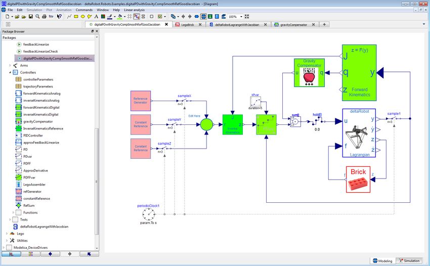
This system can be stabilized using two lead-type com-
pensators, one for each output. The first stabilizes the ball To simulate the ball maze, we require a FSM to switch
position y1 = q2 , with zero at s = −0.6, pole at s = −10 the Lagrange multipliers from active to inactive, similar to
and positive feedback gain, as shown in the root locus in Figure 1. However for the ball maze, we have sufficient
Figure 7 (top). This moves the unstable pole into the left damping to prevent bouncing, and the system will move
half plane, but leaves the two poles at the origin. After one-way through the maze, simplifying the logic. Essen-
closing this loop, we next compute the pole-zero map for tially the constraints become active when the ball contacts
the system from u2 to y2 . This shows the two poles at the a ring, i.e., when h1 changes sign, for the sequence of rings
origin and a non-minimum phase zero at s = 0.7. This can (note that h1 depends on ring radius i), and become inac-
also be stabilized with a lead compensator with zero at tive i.e., the ball falls through a gate, when the rotation of
s = −0.05, pole at s = −5.0, and gain k2 = 0.04, as shown the maze moves the gate under the ball. We can define theFigure 8. Feedback Controller for Ball Maze.
Free
Contact = 0
Ring 1 Free
Contact Gate 1
Contact = 1 Contact = 2
Ring 2 Free
Contact Gate 2
Contact = 3 Contact = 4
Ring 3 Free
Contact Gate 3
Contact = 5 Contact = 6
Goal Ring
Contact
Contact = 7
Figure 10. Ball maze simulation. Note the brevity of the free-
Figure 9. Ball maze FSM.
motion states, contact = 2, 4, 6, when the ball passes through a
gate, and when λ = 0.
location of the gates by defining
q + r atan(q2 /q3 ) − π/2 for i=1 Dymola animation of the closed-loop system. Note that
1 m1
−q1 − rm2 atan(q2 /q3 ) for i=2 we show only three rings here for simplicity. Space con-
ψ(q, i) =
q1 + rm3 atan(q2 /q3 ) − π/2 for i=3 straints prohibit a full listing of the Modelica code, which
−q − r atan(q /q ) for i=4 can be obtained by contacting the author directly. Note
1 m4 2 3
(10) that it would be simpler to rotate the maze in a single di-
so that ψ(q, i) changes sign as the ball moves “over” open rection. However, changing the direction of q̇1 allows for
gate i. Then the FSM is as shown in Figure 9, and is the maze to retain previously collected balls in the center.
straightforward to implement as a Modelica algorithm. It also shows the slower and non-minimum phase response
Figure 10 shows results of a Dymola simulation of the of the maze angle q1 to the reference.
closed-loop system. The ball is initialized in the free state,
and falls toward the outer ring, making contact at about
t = 0.1s. The maze turns counterclockwise beginning at
t = 10s and rotates until the ball falls through gate 1. As it
falls through the gate, in the contact = 2 state, λ = 0 and
the ball moves freely, until it collides with ring 2 at about
t = 22s. The collision causes the large spike in λ , repre-
senting the elastic collision, after which the contact = 3
state is maintained as the maze is rotated clockwise until
gate 2 is below the ball. Thus, as the maze rotates, the sys-
tem switches between the constrained contact state and an
unconstrained free state, although the number of dynamic
states remains constant (8) throughout. The ball maze con-
tinues to rotate until the ball gets to the inner ring, at which Figure 11. Sequence of ball maze configurations as the closed-
loop system drives the ball toward the goal.
point the controller is turned off.
Figure 11 shows a sequences of screen captures from ax1
Base
x2
x3
Proximal
Link 3
Proximal
Link 1
Distal
Distal Link 3 Link 2
Distal Link 1
Wrist Flange
Figure 12. Delta robot.
4 Delta Robot Soft-Touch Control
The delta robot (Clavel, 1990) shown in Figure 12 con-
sists of three (or more) identical under-actuated arms, ar-
ranged symmetrically about the x3 -axis (pointing down).
Each arm consists of a proximal link, rigidly attached to
the servomotor shaft at the base, and a pair of parallel dis-
tal links that are attached to the proximal link by universal
joints. The six distal links are in turn attached to the wrist
flange by universal joints, so that the two distal links as-
sociated with each arm remain parallel during operation.
The configuration provides three translation DOFs of the
wrist flange within the robot’s reachable workspace, while
the orientation of the wrist flange remains fixed. This ben-
eficial feature of the delta robot decouples the translational Figure 13. Simulation of soft collision and contact. The dis-
kinematics and dynamics of the robot from the rotational tance to the object (top), is commanded by a smooth reference to
kinematics and dynamics associated with a wrist that is be within 5mm of the object in the first 2.5s. Then it approaches
mounted below the wrist flange (not shown in Figure 12). at low velocity of 0.2mm/s, and the position gain k p is reduced
The servomotor angles are directly measured, while the continuously to zero until t = 9s. At this point the robot is in
velocity control mode. Contact is made at t = 12s, and the force
universal joint angles are not measured, but can be com-
of impact peaks at 90mN, below what would cause the block to
puted from the servomotor angles via the forward kine- move. Contact is maintained with a force of 40mN, and there is
matics. no motion of the block or bouncing.
A formulation and Modelica realization of the delta
robot translational dynamics was derived previously
(Bortoff, 2018, 2019) by defining the dynamics for low velocity and low impedance so that it does not trans-
each unconstrained arm, and then adding the holonomic fer energy sufficient to cause motion of the block. For this
coupling constraint representing the connections to the particular simulation, the gripper servo is not used.
wrist flange. The resulting index-3 differential-algebraic Figure 14 is a block diagram in Dymola showing the
equation (DAE) is stabilized using Baumgarte’s method feedback controller. The reference generator computes
(Baumgarte, 1972, 1983), giving an index-1 DAE. smooth reference trajectories for position, velocity and ac-
The objective here is to derive and simulate a soft- celeration in task space within constraints on maximum
values for velocity, acceleration and jerk, using cubic
contact control algorithm for the delta robot. In this case
splines. In this specific case, the trajectory is such that
the task object is a Lego brick on a surface, and the task is the approach velocity is 0.2mm/s. The PDFF controller
to pick up the brick with a gripper that is mounted to the block is a digital PD controller with feedforward
wrist flange without sliding the brick along the surface,
despite uncertainty in its location on the surface. Such a u(k) = k p (k)(r(k) − y(k)) + kd (k)(ṙ(k) − ẏ(k)) + r̈(k) + f (k)
control algorithm would be used in practice to grasp very (11)
fragile objects. To accomplish this, the gripper frame is where ẏ(k) is computed by filtering y(k) to approximate
moved by the robot servos so that the left finger is close the derivative, the feedback gains k p and kd are time-
to the block surface, and then it approaches the block with varying, set by a higher-level controller, and f is an ex-Figure 14. Feedback control model for soft contact. Blocks in green are discrete-time control blocks that use the Modelica Syn-
chronous Library and compute forward and inverse kinematics, PD control with variable gains, and gravity torque compensation.
The pink blocks at left compute smooth reference trajectories. The red Brick block computes the dynamics of a block in contact
with a surface, which comes in contact with the delta robot end effector during simulation. The input f into the delta robot model
is the force applied to the end effector by the brick, which is a Lagrange multiplier internal to the Brick model. Our deltaRobot
library is open at right, showing some of the control system components.
ternal input from the left touch sensor, which is not used contact without any switch. This is important because we
here. The Forward and Inverse Kinematics blocks, and the want to eliminate tuning and commissioning effort, and
Gravity Compensator block, compute the forward and in- we desire a control architecture amenable to robustness
verse kinematics, and also a torque to cancel the effect of analysis.
gravity on the robot. These functions cannot be computed Figure 13 shows a simulation result of the end effec-
analytically for the delta robot, and use Newton’s method tor approaching and contacting the brick. The contact be-
to solve a set of implicit functions, described in (Bortoff, tween the block and surface, and between the block and
2018). robot is modeled as in Section 2. In this simulation, a
To achieve soft contact, the k p gain in the direction of smooth trajectory commands the left finger to approach at
travel is continuously reduced to zero as it approaches low velocity, while the impedance is reduced by contin-
the brick, putting the robot effectively in velocity control uously until k p = 0 before impact. From this point for-
mode and reducing its impedance at the moment of con- ward it is effectively in a velocity control mode. Contact
tact. Closed-loop stability is maintained if is made, and the Lagrange multiplier becomes active at
t = 12s. There is no bounce and the force imparted is
0 ≤ k p (k) ≤ kd2 , (12) sufficiently small to maintain the friction contact with the
surface, so the block does not move. The small force is
for fixed kd , which follows from the Circle criteria maintained after the contact.
(Vidyasagar, 1993). Importantly, there is no heuristic
switch from a “position control mode” to a “velocity con- 5 Conclusions
trol mode.” Rather it is a single controller that is continu-
ously adjusted between these two extremes along the ref- We have presented a useful model of contact and colli-
erence trajectory as the end effector approaches the task sion intended to support development of model-based con-
object. Further, there is no switch from “motion control trol design and analysis for robotic assembly. The advan-
mode” to a “force control mode” when contact is detected. tages and disadvantages of the modeling approach were
In fact, the robot lacks a force - torque sensor. Rather, discussed. In particular, this method will be effective in
there is a single feedback controller that can achieve soft situations involving low numbers of contacts, where it isimportant to enforce penetration constraints after the colli- Martin Otter, Hilding Elmqvist, and José Díaz López. Collision
sion transient occurs, and in cases where dynamic analysis handling for the Modelica MultiBody library. In Proceedings
is required, not just time-domain simulation. Three exam- of the 4th International Modelica Conference, pages 45–53,
ples illustrate the method, with the ball maze providing a March 2005.
control design and simulation use case. In the future we Bernhard Thiele, Thomas Beutlich, Volker Waurich, Martin
intend to use this method to develop a range of control al- Sjölund, and Tobias Belmann. Towards a standard-comform,
gorithms for robotic assembly, in addition to mechatronic platform-generic and feature-rich Modelica device drivers li-
problems in which contact and collisions are central to the brary. In Proceedings of the 12th International Modelica
problem. Conference, pages 713–723, 2017.
References Jeroen van Baar, Alan Sullivan, Radu Cordorel, Davesh Jha,
Diego Romeres, and Daniel Nikovski. Sim-to-real transfer
Gianluca Bardaro, Luca Bascetta, Francesco Casella, and Mat- learning using robustified controllers in robotic tasks involv-
teo Matteucci. Using Modelica for advanced multi-body ing complex dynamics. In Proceedings of the IEEE Interna-
modelling in 3D graphical robotic simulators. In Proceed- tional Conference on Robotics and Automation, 2019.
ings of the 12th International Modelica Conference, pages
887–894, 2017. M. Vidyasagar. Nonlinear Systems Analysis: Second Edition.
Prentice-Hall, 1993.
J. W. Baumgarte. Stabilization of constraints and integrals of
motion in dynamic systems. Computer Methods in Applied Miomir Vukobratovic, Veljko Potkonjak, and Vladimir Matije-
Mechanics and Engineering, 1:1–16, 1972. vic. Dynamics of Robots with Contact Tasks. Kluwer, 2003.
J. W. Baumgarte. A new method of stabilization for holonomic
constraints. ASME Journal of Applied Mechanics, 50:869–
870, 1983.
Scott A. Bortoff. Object-oriented modeling and control of delta
robots. In IEEE Conference on Control Technology and Ap-
plications, pages 251–258, 2018.
Scott A. Bortoff. Using Baumgarte’s method for index reduc-
tion in Modelica. In Proceedings of the 13th International
Modelica Conference, pages 333–342, March 2019.
R. Clavel. Device for the movement and positioning of an ele-
ment in space. U.S. Patent 4, 976, 582, Dec. 11 1990.
Erwin Coumans. Bullet 2.83 physics SDK manual.
https://github.com/bulletphysics/bullet3/tree/master/docs,
2015.
Vadim Engelson. Integration of Collision Detection with
the Multibody System Library in Modelica. PhD thesis,
Link oping University, 2000.
Kenny Erleben, Jon Sporring, Knud Henriksen, and Henrik
Dohlmann. Physics-Based Animaation. Charles River Me-
dia, 2005.
Elmer Gilbert, Daniel W. Johnson, and S. Sathiya Keerthi. A
fast procedure for compting the distance bewteen complex
objects in three-dimensional space. IEEE Journal of Robotics
and Automation, 4(2):193–203, 1988.
Andreas Hofmann, Lars Mikelsons, Ines Gubsch, and Christian
Schubert. Simulating collisions within the Modelica multi-
body library. In Proceedings of the 10th International Mod-
elica Conference, pages 949–957, 2011a.
Andreas Hofmann, Lars Mikelsons, Ines Gubsch, and
Christian Schubert. Modelica idealized contact library.
https://github.com/modelica-3rdparty/IdealizedContact,
2011b.You can also read