What are you talking about? Text-to-Image Coreference
←
→
Page content transcription
If your browser does not render page correctly, please read the page content below
What are you talking about? Text-to-Image Coreference
Chen Kong1 Dahua Lin3 Mohit Bansal3 Raquel Urtasun2,3 Sanja Fidler2,3
1
Tsinghua University, 2 University of Toronto, 3 TTI Chicago
kc10@mails.tsinghua.edu.cn, {dhlin,mbansal}@ttic.edu,{fidler,urtasun}@cs.toronto.edu
Abstract
In this paper we exploit natural sentential descriptions
of RGB-D scenes in order to improve 3D semantic parsing.
Importantly, in doing so, we reason about which particular
object each noun/pronoun is referring to in the image. This
allows us to utilize visual information in order to disam-
biguate the so-called coreference resolution problem that
arises in text. Towards this goal, we propose a structure
prediction model that exploits potentials computed from text
and RGB-D imagery to reason about the class of the 3D ob-
jects, the scene type, as well as to align the nouns/pronouns
with the referred visual objects. We demonstrate the effec-
tiveness of our approach on the challenging NYU-RGBD v2
dataset, which we enrich with natural lingual descriptions.
We show that our approach significantly improves 3D de-
tection and scene classification accuracy, and is able to re-
liably estimate the text-to-image alignment. Furthermore,
by using textual and visual information, we are also able to
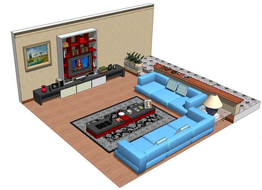
successfully deal with coreference in text, improving upon Figure 1. Our model uses lingual descriptions (a string of depen-
the state-of-the-art Stanford coreference system [15]. dent sentences) to improve visual scene parsing as well as to de-
termine which visual objects the text is referring to. We also deal
with coreference within text (e.g., pronouns like “it” or “them”).
1. Introduction
Imagine a scenario where you wake up late on a Satur- system is key for the deployment of such systems. To date,
day morning and all you want is for your personal robot to however, attempts to utilize more complex natural descrip-
bring you a shot of bloody mary. You could say “It is in the tions are rare. This is due to the inherent difficulties of both
upper cabinet in the kitchen just above the stove. I think it is natural language processing and visual recognition, as well
hidden behind the box of cookies, which, please, bring to me as the lack of datasets that contain such image descriptions
as well.” For a human, finding the mentioned items based linked to visual annotations (e.g., segmentation, detection).
on this information should be an easy task. The description Most recent approaches that employ text and images fo-
tells us that there are at least two cabinets in the kitchen, one cus on generation tasks, where given an image one is inter-
in the upper part. There is also a stove and above it is a cab- ested in generating a lingual description of the scene [8, 12,
inet holding a box and the desired item should be behind it. 21, 2], or given a sentence, retrieving related images [29].
For autonomous systems, sentential descriptions can serve An exception is [9], which employed nouns and preposi-
as rich source of information. Text can help us parse the tions extracted from short sentences to boost the perfor-
visual scene in a more informed way, and can facilitate for mance of object detection and semantic segmentation.
example new ways of active labeling and learning. In this paper we are interested in exploiting natural lin-
Understanding descriptions and linking them to visual gual descriptions of RGB-D scenes in order to improve 3D
content is fundamental to enable applications such as se- object detection as well as to determine which particular
mantic visual search and human-robot interaction. Using object each noun/pronoun is referring to in the image. In
language to provide annotations and guide an automatic order to do so, we need to solve the text to image alignment
1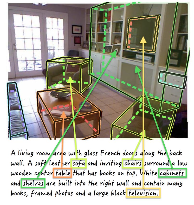
problem, as illustrated with the arrows in Fig. 1. Towards       tion recognition. We expect the dataset we collect here to
this goal, we propose a holistic model that reasons jointly      be of great use to both the NLP and vision communities.
about the visual scene and as well as text that accompanies
the image. Our model is a Markov Random Field (MRF)              3. Text to Image Alignement Model
which reasons about the type of scene, 3D detection as well
as to which visual concept each noun/pronoun refers to. We           Our input is an RGB-D image of an indoor scene as well
demonstrate the effectiveness of our approach in the chal-       as its multi-sentence description. Out goal is to jointly parse
lenging NYU-RGBD v2 dataset [27] which we enrich with            the 3D visual scene and the text describing the image, as
natural lingual descriptions. Our model is able to signif-       well as to match the text to the visual concepts, perform-
icantly improve 3D detection and scene classification ac-        ing text to image alignment. We frame the problem as the
curacy over the visual-only baseline. Furthermore, it suc-       one of inference in a Markov Random Field (MRF) which
cessfully deals with the text to image alignment problem, as     reasons about the type of scene, 3D detection as well as for
well as with coreference resolution in text, improving over      each noun/pronoun of interest which visual concept it cor-
the state-of-the-art Stanford coreference system [15].           respond to. To cope with the exponentially many detection
                                                                 candidates we use bottom-up grouping to generate a smaller
                                                                 set of “objectness” cuboid hypothesis, and restrict the MRF
2. Related Work
                                                                 to reason about those. In the following, we describe how
    There has been substantial work in automatic caption-        we parse the text in Sec. 3.1, generate 3D object candidates
ing or description generation of images [12, 13, 14] and         in Sec 3.2, and explain our MRF model in Sec. 3.3.
video [2]. Text has also been used as a form of weak
supervision to learn visual models. In [35], representa-         3.1. Parsing Textual Descriptions
tions for word meanings are learned from short video clips           We extract part of speech tags (POS) of all sentences in
paired with sentences by learning the correspondence be-         a description using the Stanford POS Tagger for English
tween words and video concepts in an unsupervised fash-          language [31]. Type dependencies were obtained using [6].
ion. Ramanathan et al. [23] use textual descriptions of          Nouns: We extract nouns from the POS, and match them
videos to learn action and role models. Matuszek et al. [19]     to the object classes of interest. In order to maximize the
jointly learn language and perception models for grounded        number of matched instances, we match nouns not only to
attribute induction. In [10], prepositional relations and        the name of the class, but also to its synonyms and plural
adjectives are used to learn object detection models from        forms. We obtain the synonyms via WordNet as well as
weakly labeled data. Natural descriptions have also recently     from our text ground-truth (GT). In particular, we add to
been used as semantic queries for video retrieval [17].          our list of synonyms all words that were annotated as object
    Very little work has been devoted to exploiting text to      class of interest in the training split of the text GT.
improve semantic visual understanding beyond simple im-
                                                                 Attributes: To get attributes for a noun we look up all
age classification [22], or tag generation [7, 3]. Notable
                                                                 amod and nsubj that modify a noun of interest in Stan-
exceptions are [16, 28], which exploit weak labels in the
                                                                 ford’s parser dependency information. Here amod means
form of tags to learn models that reason about classifica-
                                                                 an adjectival modifier, e.g., amod(brown, table), and nsubj
tion, annotation as well as segmentation. The work closest
                                                                 is a nominal subject, e.g. for “The table is brown” we
to us is [9], where short sentences are parsed into nouns
                                                                 have nsubj(brown,table). The parser can handle multiple
and prepositions, which are used to generate potentials in
                                                                 attributes per noun, which we exploit.
a holistic scene model [34]. However, the approach does
not identify which instance the sentence is talking about,       Pronouns: Since the sentences in our descriptions are not
and for example whenever a sentence mentions a “car”, the        independent but typically refer to the same entity multiple
model boosts all car hypotheses in the image. In contrast,       times, we are faced with the so-called coreference resolu-
here we are interested in aligning nouns and pronouns in         tion problem. For example, in “A table is in the room. Next
text with the referred objects in the image. Further, in our     to it is a chair.”, both table and it refer to the same ob-
work we use complex natural descriptions composed of sev-        ject and thus form a coreference. To address this, we use
eral sentences, as opposed to single sentences used in [9],      the Stanford coreference system [15] to predict clusters of
where additional challenges such as coreference emerge.          coreferrent mentions. This is a state-of-the-art, rule-based
    Only a few datasets contain images and text. The UIUC        and sieve-based system which works well on out-of-domain
dataset [8] augments a subset of PASCAL’08 with 3 inde-          data. We generate multiple coreference hypotheses1 in or-
pendent sentences (each by a different annotator) on aver-       der to allow the MRF model to correct for some of the coref-
age per image, thus typically not providing very rich de-        erence mistakes using both textual and visual information.
scriptions. Other datasets either do not contain visual labels     1 We ran [15] with different values of maxdist parameter which is the

(e.g., Im2Text [21]) or tackle a different problem, e.g., ac-    maximum sentence distance allowed between two mentions for resolution.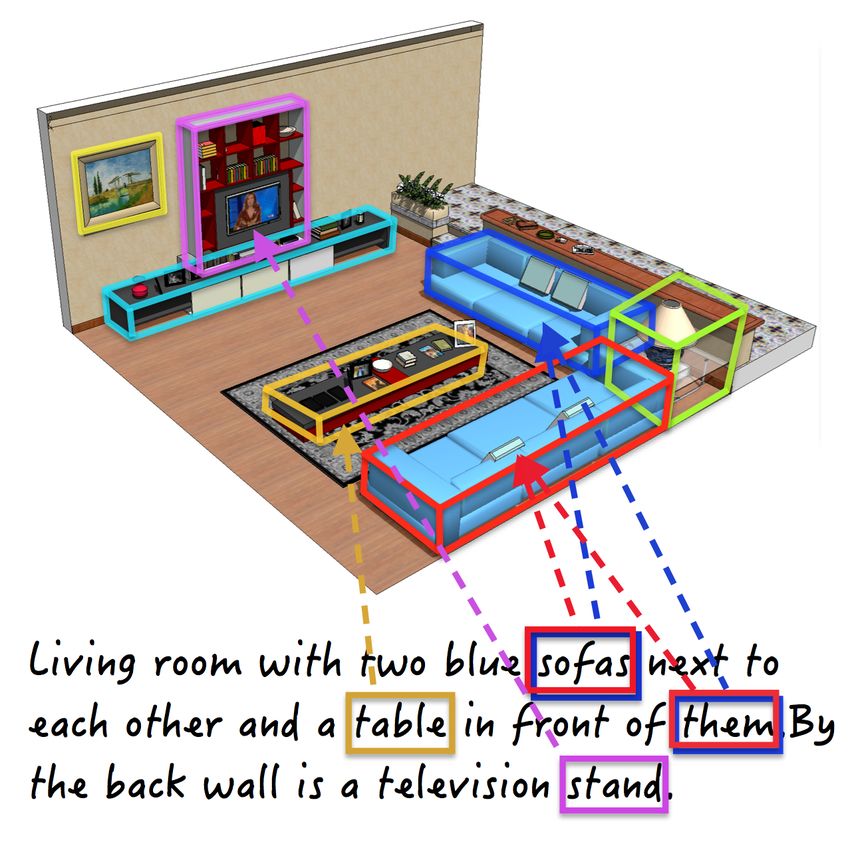
text
                                            a,a
                        a(1)                      a(2)
            text,rgbd          a,o                           text,rgbd                   MRF energy sums the energy terms exploiting the image
    scene               a,o
                                                    a,o
                                                                                         and textual information while reasoning about the text to
  (e.g. “living room”)                                    sofa
                                                                                         image alignment. The graphical model is depicted in Fig. 2.
                                                          bed
                                                                                         We now describe the potentials in more detail.
    cuboids                                          cabinet
                                                                 liv       b   k
                                                                       . r edr itch
                                                                          o o o om e n   3.3.1   Visual Potentials
                                                                             m

                                                                                         Our visual potentials are based on [18] and we only briefly
                                                                                         describe them here for completeness.
                                        “Living room with two blue
                                                                                         Scene Appearance: To incorporate global information
                                        sofas next to each other and a
                                        table in front of them. By the                   we define a unary potential over the scene label, computed
                                        back wall is a television stand.”                by means of a logistic on top of a classifier score [33].
                                                                                         Cuboid class potential: We employ CPMC-o2p [4] to
Figure 2. Our model. Black nodes and arrows represent visual                             obtain detection scores. For the background class, we use
information [18], blue are text and alignment related variables.                         a constant threshold. We use an additional classifier based
                                                                                         on the segmentation potentials of [24], which classify su-
   Pronouns are tagged as PRP by the Stanford parser. We                                 perpixels. To compute our cuboid scores, we compute the
take all PRP occurrences that are linked to a noun of interest                           weighted sum of scores for the superperpixels falling within
in our coreference clusters. We extract attributes for each                              the convex hull of the cuboid in the image plane.
such pronoun just as what we do for a noun.                                              Object geometry: We capture object’s geometric proper-
                                                                                         ties such as height, width, volume, as well as its relation to
3.2. Visual Parsing                                                                      the scene layout, e.g., distance to the wall. We train an SVM
    Our approach works with a set of object candidates rep-                              classifier with an RBF kernel for each class, and use the re-
resented as 3D cuboids and reasons about the class of each                               sultant scores as unary potentials for the candidate cubes.
cuboid within our joint visual and textual MRF model. We                                 Semantic context: We use two co-occurrence relation-
follow [18] to get cuboid candidates by generating ranked                                ships: scene-object and object-object. The potential values
3D “objectness” regions that respect intensity and occlusion                             are estimated by counting the co-occurrence frequencies.
boundaries in 3D. To get the regions we use CPMC [5] ex-                                 Geometric context: We use two potentials to exploit the
tended to 3D [18]. Each region is then projected to 3D via                               spatial relations between cuboids in 3D, encoding close-to
depth and a cuboid is fit around it by requiring the horizon-                            and on-top-of relations. The potential values are simply the
tal faces to be parallel to the ground. In our experiments,                              empirical counts for each relation.
we vary the number K of cuboid hypotheses per image.
                                                                                         3.3.2   Text-to-Image Alignment Potentials
3.3. Our Joint Visual and Textual Model
                                                                                         A sentence describing an object can carry rich information
    We define a Markov Random Field (MRF) which rea-                                     about its properties, as well as 3D relations within the scene.
sons about the type of scene, 3D detection as well as for                                For example, a sentence “There is a wide wooden table by
each noun/pronoun of interest which visual concept it cor-                               the left wall.” provides size and color information about the
respond to. More formally, let s ∈ {1, . . . , S} be a ran-                              table as well as roughly where it can be found in the room.
dom variable encoding the type of scene, and let yi ∈                                    We now describe how we encode this in the model.
{0, · · · , C}, with i = 1, · · · , K, be a random variable asso-                        Scene from Text: In their description of the image, peo-
ciated with a candidate cuboid, encoding its semantic class.                             ple frequently provide information about the type of scene.
Here yi = 0 indicates that the cuboid is a false positive.                               This can be either direct, e.g., “This image shows a child’s
Let T be the textual information and let I be the RGB-D                                  bedroom.”, or indirect “There are two single beds in this
image evidence. For each noun/pronoun corresponding to                                   room”. We encode this with the following potential:
a class of interest we generate an indexing random variable
aj ∈ {0, · · · , K} that selects the cuboid that the noun refers                                           φscene (s = u|T ) = γu ,                 (1)
to. The role of variables {aj } is thus to align text with visual
objects. Note that aj = 0 means that there is no cuboid cor-                             where γu is the score of an SVM classifier (RBF kernel). To
responding to the noun. This could arise in cases where our                              compute its features, we first gathered occurrence statistics
set of candidate cuboids does not contain the object that the                            for words in the training corpus and took only words that
noun describes, or the noun refers to an virtual object that is                          exceeded a minimum occurrence threshold. We did not use
in fact not visible in the scene. For plural forms we generate                           stop words such as and or the. We formed a feature vec-
as many a variables as the cardinality of the (pro)noun. Our                             tor with an 0/1 entry for each word, depending whether the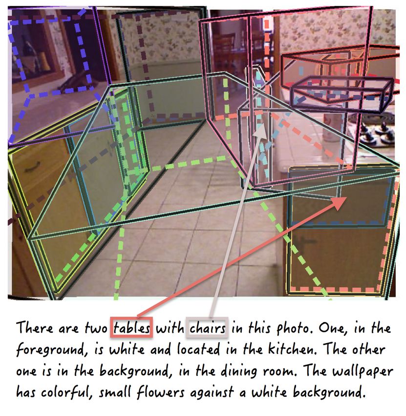
mantel counter toilet   sink bathtub bed headb. table shelf   cabinet sofa   chair chest refrig. oven microw. blinds curtain board monitor printer
% mentioned 41.4 46.4 90.6          78.2 55.6 79.4 9.2 53.4 32.9           27.7 51.2     31.6 45.7 55.7 31.4 56.0 26.2 23.0 28.6 66.7 44.3
  # nouns    19      948 120        219 84 547 7 1037 240                  1105 375       631 131 68 57             46      41     74     64    226      58
 # of coref   3      71     28       49    11 145 0          212 27         129 80         57    8      7     7     11       1      2      8     29       8
Table 1. Dataset statistics. First row: Number of times an object class is mentioned in text relative to all visual occurrences of that class.
Second row: The number of noun mentions for each class. Third row: Number of coreference occurrences for each class.

description contained the word or not. For nouns referring                       training examples for (size,class) pairs, we add another fea-
to scene types we merged all synonym words (e.g., “dining                        ture to the classifier which is 1 if the noun comes from a
room”, “dining area”) into one entry of the feature vector.                      group of big objects (e.g., bed, cabinet) and 0 otherwise.
Alignment: This unary potential encodes the likelihood                           Text-cuboid Compatibility: This potential ensures that
that the j-th relevant noun/pronoun is referring to the i-th                     the class of the cuboid that a particular aj selects matches
cuboid in our candidate set. We use the score of a classifier,                   the aj ’s noun. We thus form a noun-class compatibility po-
                                                                                 tential between aj and each cuboid:
             φalign
              ao (aj = i|I, T ) = score(aj , i),                     (2)
                                                                                            φcompat.
                                                                                             ao      (aj = i, yi = c) = stats(class(j), c)                (4)
which exploits several visual features representing the i-th                     When aj corresponds to a pronoun we find a noun from
cuboid, such as its color, aspect ratio, distance to wall, and                   its coreference cluster and take its class. We use empiri-
textual features representing information relevant to aj ’s                      cal counts as our potential rather than a hard constraint as
noun, such as “wide”, “brown”, “is close to wall”. On the                        people confuse certain types of classes. This is aggravated
visual side, we use 10 geometric features to describe each                       by the fact that our annotators were not necessarily native
cuboid (as in Sec. 3.3.1), as well as the score of a color clas-                 speakers. For example people would say “chest” instead of
sifier for six main colors that people most commonly used                        “cabinet”. These errors are challenges of natural text.
in their descriptions (white, blue, red, black, brown, bright).                  Variety: Notice that our potentials so far are exactly the
To exploit rough class information we also use the cuboid’s                      same for all aj corresponding to the same plural mention,
segmentation score (Sec. 3.3.1). Since people typically de-                      e.g., “Two chairs in the room.” However, since they are re-
scribe more salient objects (bigger and image centered), we                      ferring to different objects in the scene we encourage them
use the dimensions of the object’s 2D bounding box (a box                        to point to different cuboids via a pairwise potential:
around the cuboid projected to the image), and its x and y                                                         (
image coordinates as additional features. We also use the                                    variety                 −1 if aj = ak
                                                                                           φa,a (aj , ak |T ) =                           (5)
center of the cuboid in 3D to capture the fact that people                                                           0    otherwise
tend to describe objects that are closer to the viewer.
                                                                                 3.4. Learning and Inference
    On the text side, we use a class feature which is 1 for aj ’s
noun’s class and 0 for other object classes of interest. We                         Inference in our model is NP-hard. We use distributed
also use a color feature, which is 1 if the noun’s adjective                     convex belief propagation (DCBP) [25] to perform approx-
is a particular color, and 0 otherwise. To use information                       imate inference. For learning the weights for each potential
about the object’s position in the room, we extract 9 geo-                       in our MRF, we use the primal-dual method of [11], specif-
metric classes from text: next-to-wall, in-background, in-                       ically, we use the implementation of [26].
foreground, middle-room, on-floor, on-wall, left-side-room,                         We define the loss function as a sum of unary and pair-
right-side-room, in-corner-room, with several synonyms for                       wise terms. In particular, we define a 0-1 loss over the scene
each class. We form a feature that is 1 if the sentence with                     type, and a 0-1 loss over the cuboid detections [18]. For the
aj mentions a particular geometric class, and 0 otherwise.                       assignment variables aj we use a thresholded loss:
We train an SVM classifier (RBF kernel) and transform the
                                                                                                           (
                                                                                                            1 if IOU(aj , aˆj ) ≤ 0.5
scores via a logistic function (scale 1) to form the potentials.                          ∆a (aj , âj ) =                                  (6)
                                                                                                            0 otherwise
Size: This potential encodes how likely the j-th relevant
noun/pronoun refers to the i-th cuboid, given that it was                        which penalizes alignments with cuboids that have less than
mentioned to have a particular physical size in text:                            50% overlap with the cuboids in the ground-truth align-
                                                                                 ments. For plural forms, the loss is 0 if aj selects any of
  φsize
   ao (aj = i|I, T , size(j) = sz) = scoresz (class(j), i)
                                                                                 the cuboids in the noun’s ground-truth alignment. In order
                                                           (3)                   to impose diversity, we also use a pairwise loss requiring
We train a classifier for two sizes, big and small, using geo-                   that each pair (aj , ak ), where aj and ak correspond to dif-
metric features such as object’s width and height in 3D. We                      ferent object instances for a plural noun mention, needs to
use several synonyms for both, including e.g. double, king,                      select two different cuboids: (
single, typical adjectives for describing beds. Note that size                                                     1 if aj = ak
                                                                                             ∆plural (aj , ak ) =                          (7)
depends on object class: a “big cabinet” is not of the same                                                        0 otherwise
physical size as a “big mug”. Since we do not have enough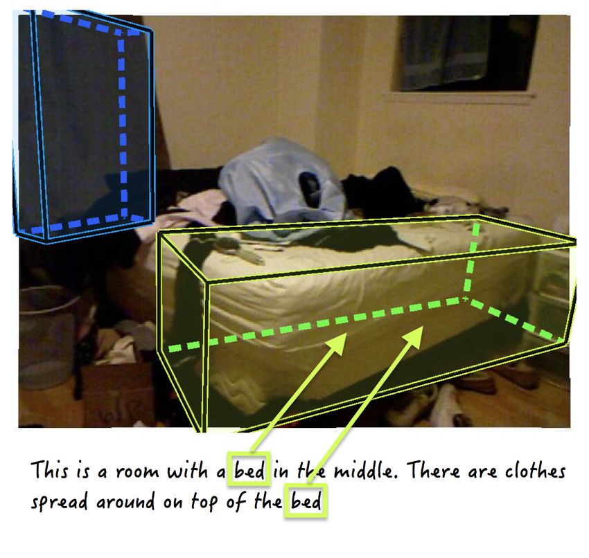
# sent # words min # sent max sent min words max words precision recall F-measure
3.2 39.1 1 10 6 144 object class 94.7% 94.2% 94.4%
# nouns of interest # pronouns # scene mentioned scene correct scene 85.7% 85.7% 85.7%
3.4 0.53 0.48 83% color 64.2% 93.0% 75.9%
size 55.8% 96.0% 70.6%
Table 2. Statistics per description.
Table 3. Parser accuracy (based on Stanford’s parser [31])
kitchen .93 0.0 .01 .01 0.0 0.0 0.0 .02 0.0 0.0 0.0 .04
office .04 .65 0.0 .04 0.0 0.0 .12 0.0 0.0 .15 0.0 0.0 MUC B3
bathroom 0.0 0.0 1.0 0.0 0.0 0.0 0.0 0.0 0.0 0.0 0.0 0.0
living r. .12 0.0 0.0 .77 .02 0.0 0.0 .05 0.0 0.0 .01 .02
Method precision recall F1 precision recall F1
bedroom 0.0 0.0 .01 .02 .94 0.0 0.0 .02 0.0 0.0 .01 0.0 Stanford [15] 61.56 62.59 62.07 75.05 76.15 75.59
bookstore 0.0 0.0 0.0 0.0 0.0 1.0 0.0 0.0 0.0 0.0 0.0 0.0
classroom 0.0 0.0 0.0 0.0 0.0 0.0 .95 0.0 .05 0.0 0.0 0.0
Ours 83.69 51.08 63.44 88.42 70.02 78.15
home off. 0.0 .66 0.0 .16 0.0 0.0 0.0 .06 0.0 0.0 .12 0.0 Table 4. Co-reference accuracy of [15] and our model.
playroom .08 0.0 0.0 .42 .17 0.0 0.0 0.0 .33 0.0 0.0 0.0
reception 0.0 .38 0.0 .25 0.0 0.0 0.0 0.0 0.0 .38 0.0 0.0
study
dining r.
.14 .71 0.0 .14 0.0 0.0 0.0 0.0 0.0 0.0 0.0 0.0
tributes for the linked pronouns as well. Our annotation
.13 0.0 0.0 .05 0.0 0.0 0.0 0.0 0.0 0.0 .05 .76
was semi-automatic, where we generated candidates using
ki
of
ba
li
be
bo
cl
ho
pl
re
st
di
tc
fi
t
vi
d
ok
a
me
ay
ce
ud
ni
the Stanford parser [31, 15] and manually corrected the mis-
hr
ro
ss
he
c
n
st
r
pt
y
ng
e
o
g
o
r
of
oo
n
om
m
o
oo
i
r.
re
f.
m
on
r.
m
Figure 3. Scene classif. accuracy with respect to NYU annotation. takes. We used WordNet to generate synonyms.
We evaluate acc. only when a scene is mentioned in a description. We analyze our dataset next. Table 2 shows simple statis-
tics: there are on average 3 sentences per description where
each description has on average 39 words. Descriptions
4. RGB-D Dataset with Complex Descriptions contain up to 10 sentences and 144 words. A pronoun be-
Having rich data is important in order to enable auto- longing to a class of interest appears in every second de-
matic systems to properly ground language to visual con- scription. Scene type is explicitly mentioned in half of the
cepts. Towards this goal, we took the NYUv2 dataset [27] descriptions. Table 1 shows per class statistics, e.g. percent-
that contains 1449 RGB-D images of indoor scenes, and age of times a noun refers to a visual object with respect to
collected sentential descriptions for each image. We asked the number of all visual objects of that class. Interestingly, a
the annotators (MTurkers) to describe an image to someone “toilet” is talked about 91% of times it is visible in a scene,
who does not see it to give her/him a vivid impression of while “curtains” are talked about only 23% of times. Fig. 4
what the scene looks like. The annotators were only shown shows size histograms for the mentioned objects, where
the image and had no idea of what the classes of interest size is the square root of the number of pixels which the
were. For quality control, we checked all descriptions, and linked object region contains. We separate the statistics into
fixed those that were grammatically incorrect, while pre- whether the noun was mentioned in the first, second, third,
serving the content. The collected descriptions go beyond or fourth and higher sentence. An interesting observation
current datasets where typically only a short sentence is is that the sizes of mentioned objects become smaller with
available. They vary from one to ten sentences per anno- the sentence ID. This is reasonable as the most salient (typ-
tator per image, and typically contain rich information and ically bigger) objects are described first. We also show a
multiple mentions to objects. Fig. 6 shows examples. plot for sizes of objects that are mentioned more than once
per description. We can see that the histogram is pushed
We collected two types of ground-truth annotations. The
to the right, meaning that people corefer to bigger objects
first one is visual, where we linked the nouns and pronouns
more often. As shown in Fig. 5, people first describe the
to the visual objects they describe. This gives us ground-
closer and centered objects, and start describing other parts
truth alignments between text and images. We used in-
of the scene in later sentences. Finally, in Fig. 3 we evaluate
house annotators to ensure quality. We took a conservative
human scene classification accuracy against NYU ground-
approach and labeled only the non-ambiguous referrals. For
truth. We evaluate accuracy only when a scene is explicitly
plural forms we linked the (pro)noun to multiple objects.
mentioned in a description. While “bathroom” is always a
The second annotation is text based. Here, the anno- “bathroom”, there is confusion for some other scenes, e.g. a
tators were shown only text and not the image, and thus “playroom” is typically mentioned to be a “living room”.
had to make a decision based on the syntactic and seman-
tic textual information alone. For all nouns that refer to the 5. Experimental Evaluation
classes of interest we annotated which object class it is, tak-
ing into account synonyms. All other nouns were marked We test our model on the NYUv2 dataset augmented
as background. For each noun we also annotated attributes with our descriptions. For 3D object detection we use the
(i.e., color and size) that refer to it. We also annotated co- same class set of 21 objects as in [18], where ground-truth
referrals in cases where different words talk about the same has been obtained by robust fitting of cuboids around object
entity by linking the head (representative) noun in a descrip- regions projected to 3D via depth. For each image NYU
tion to all its noun/pronoun occurrences. We annotated at- also has a scene label, with 13 scene classes altogether.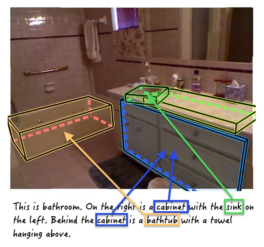
Size of objects (sent 1) Size of objects (sent 2) Size of objects (sent 3) Size of objects (sent 4) Size of multiple mentioned obj
1000 120
1200 300
400
800 1000 100 250
300
occurence
occurence
occurence
occurence
occurence
800 80 200
600
600 60 150
200
400
400 40 100
200 100
200 20 50
0 0 0 0 0
17 41 65 89 114 138 162 186 211 235 17 41 65 89 114 138 162 186 211 235 17 41 65 89 114 138 162 186 211 235 17 41 65 89 114 138 162 186 211 235 17 41 65 89 114 138 162 186 211 235
Figure 4. Statistics of sizes of described object regions give the sequential sentence number in a description.
ous work [20], the MUC metric is somewhat biased towards
large clusters, whereas the B3 metric is biased towards sin-
gleton clusters. We thus report both metrics simultaneously,
sent 1 sent 1 sent 3 sent ≥ 4 so as to ensure a fair and balanced evaluation. To compute
the metrics we need a matching between the GT and pre-
dicted mentions. We consider a GT and predicted mention
to be matched if the GT’s head-word is contained in the pre-
diction’s mention span.2 All unmatched mentions (GT and
predicted) are penalized appropriately by our metrics.3
5.2. Results
To examine the performance of our model in isolation,
we first test it on the GT cuboids. In this way, the errors
Figure 5. Top: Location statistics of mentioned objects given
introduced in the detection stage are not considered. We
which sentence mentions them. Bottom: Statistics of mentioned
objects in 3D. We translate each scene to have the ground at y = 0. measure the performance in terms of classification accu-
racy, i.e., the percentage of correctly classified objects. We
5.1. Performance metrics consider various configurations of our model that incorpo-
rate different subsets of potentials, so as to analyze their
Cuboid: An object hypotheses is said to be correct if it
individual effect. The results are presented in Table 5. By
overlaps with a ground-truth object (of the same class) more
“+” we denote that we added a potential to the setting in the
than 50% IOU. Detector’s performance is then measured in
previous line. Here “a coref” denotes that we used the a
terms of the F-measure averaged across the classes.
variables also for the coreferred words (see Sec. 3.1) as op-
Text-cuboid alignment: We say that an alignment aj = i
posed to just for the explicit noun mentions. We can observe
is correct if IOU between the i-th candidate cuboid and the
that overall our improvement over the visual-only model is
cuboid in aj ’s GT alignment is higher than 50%. For plural
significant, 14.4% for scene classification and 6.4% for ob-
nouns with several {ajk }, we take an union of all cuboids ik
ject detection. Further, the full model improves 2.3% over
in the inferred alignments: ajk = ik . We compute IOU be-
the unary-based alignment when evaluating nouns only (de-
tween this union and the union of cuboids in the GT align-
noted with align N in the Table) as well as for both nouns
ment for this noun. We evaluate via F-measure. We use
and pronouns (denoted with align N+P).
two metrics, one for all alignments in our GT, including
For real cuboids, we test our performance by varying the
nouns/pronouns, and one for only the alignment of nouns.
number K of cuboid hypotheses per scene. The results are
Scene: Accuracy is computed as the average along the di-
shown in Table 5 showing that performance in all tasks im-
agonal of the confusion matrix.
proves more than 5% over the baseline. The joint model
Text parser: In order to understand the performance of
also boosts the text to cuboid alignment performance over
our model, it is important to sanity check the performance
unary only (which can be considered as an intelligent text-
of the Stanford-based text parser in our setting. The results
visual baseline), most notably for K = 15. Performance
are shown in Table 3 in terms of F-measure. We can see that
for each class is shown in Table 6, showing a big boost in
while the object and scene performance is relatively good,
accuracy for certain classes. Note that for GT cuboids, Ta-
parsing of the attributes is legging behind.
ble 5 shows classification accuracy, while Table 6 shows
Coreference metrics: We evaluate the predicted corefer- F-measure. For real cuboids both tables show F-measure.
ence clusters with MUC [32] and B3 [1] metrics. MUC Note that our model can also re-reason about coreference
is a link-based metric that measures how many predicted in text by exploiting the visual information. This is done via
mention clusters need to be merged to cover the gold (GT)
2 This is because we start with “visual” head-words as the gold-standard
clusters. B3 is a mention-based metric which computes pre-
mentions. In case of ties, we prefer mentions which are longer (if they have
cision and recall for each mention as the overlap between the same head-word) or closer to the head-word of the matching mention.
its predicted and gold cluster divided by the size of the pre- 3 We use a version of the B3 metric called B3 all, defined by [30] that
dicted and gold cluster, respectively. As shown by previ- can handle (and suitably penalize) unmatched GT and predicted mentions.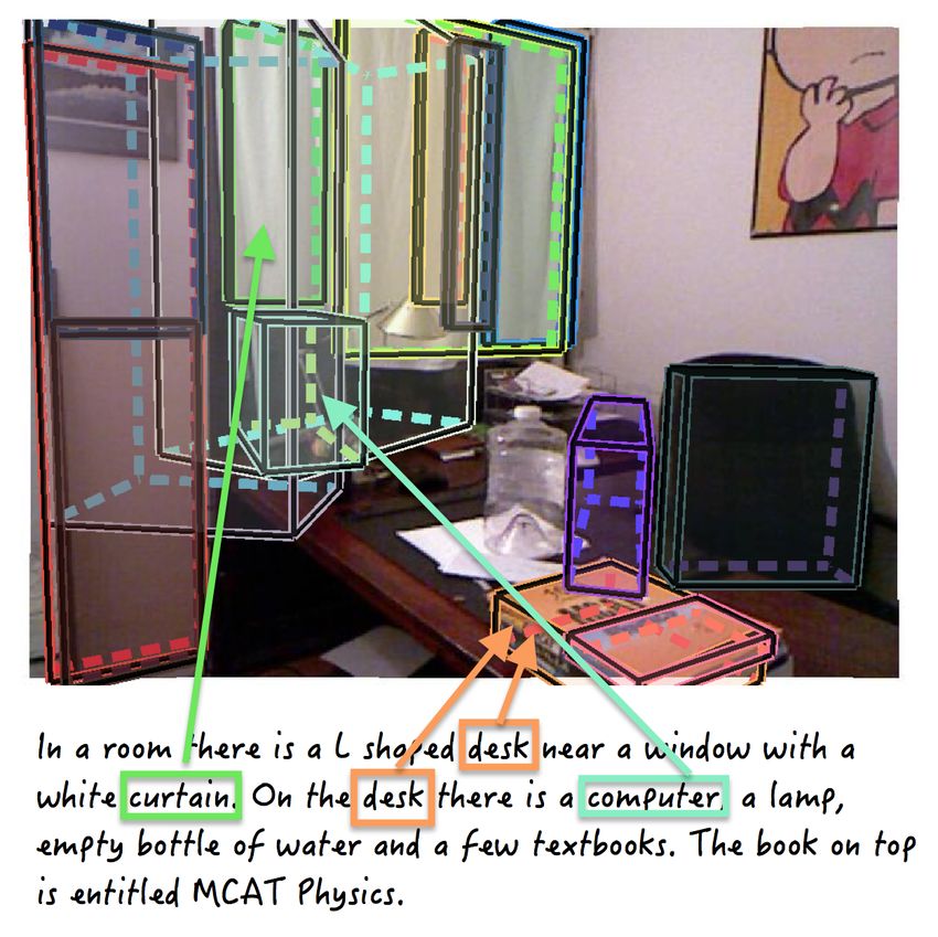
Ground-truth cuboids                     our cuboids (K = 8)                   our cuboids (K = 15)
                    scene    object align. N align N+P       scene   object align N align N+P      scene    object align N align N+P
  [18]              58.1    60.5        –          –        38.1     44.3     –          –      54.4   37.3       –         –
 random assign.      –        –       15.8       15.3         –       –      5.9        5.7      –      –        4.7       4.6
 assign. to bckg.    –        –        7.5        7.3         –       –      7.7        7.5      –      –        7.7       7.5
 + scene text       67.1    60.7        –          –        62.4     44.3     –          –      61.6   37.3       –         –
 + a unary          67.1    60.6      51.4       49.7       62.5     44.3   20.4       19.8     60.9   37.3     20.4      19.7
 + a size           67.1    60.6      51.6       49.9       62.5     44.3   20.4       19.7     60.9   37.3     20.4      19.8
 + a-to-cuboid      72.2    66.8      53.2       51.5       67.0     49.1   24.0       23.2     61.9   43.5     24.8      24.0
 + a coref          72.3    67.1      53.6       51.8       67.1     48.8   23.5       22.7     61.9   43.4     24.9      24.1
 + a variability    72.5    67.0      53.7       52.0       67.1     48.7   23.5       22.8     61.6   44.1     25.1      24.3
Table 5. Results with the baseline and various instantiations of our model. Here assign N means noun-cuboid assignment accuracy (F
measure), and assign N+P where we also evaluate assignment of pronouns to cuboids. K means the number of cuboid candidates used.

the inferred {aj } variables: each aj in our MRF selects a               [6] M. de Marneffe, B. MacCartney, and C. Manning. Gener-
cuboid which the corresponding (pro)noun talks about. We                     ating typed dependency parses from phrase structure parses.
then say that different a variables selecting the same cuboid                In LREC, 2006. 2
form a coreference cluster. Table 4 shows the accuracy of                [7] P. Duygulu, K. Barnard, N. de Freitas, and D. Forsyth. Object
the Stanford’s coreference system [15] and our approach.                     recognition as machine translation: Learning a lexicon for a
Note that in our evaluation we discard (in Stanford’s and                    fixed image vocabulary. In ECCV, 2002. 2
our output) all predicted clusters that contain only non-gold            [8] A. Farhadi, M. Hejrati, M. Sadeghi, P. Young, C. Rashtchian,
                                                                             J. Hockenmaier, and D. Forsyth. Every picture tells a story:
mentions. This is because our ground-truth contains coref-
                                                                             Generating sentences for images. In ECCV, 2010. 1, 2
erence annotation only for 21 classes of interest, and we do
                                                                         [9] S. Fidler, A. Sharma, and R. Urtasun. A sentence is worth a
not want to penalize precision outside of these classes, espe-
                                                                             thousand pixels. In CVPR, 2013. 1, 2
cially for the Stanford system which is class agnostic. Our
                                                                        [10] A. Gupta and L. Davis. Beyond nouns: Exploiting prepo-
results show that we can improve over a text-only state-of-                  sitions and comparative adjectives for learning visual classi-
the-art system [15] via a joint text-visual model. This is, to               fiers. In ECCV, 2008. 2
the best of our knowledge, the first result of this kind.               [11] T. Hazan and R. Urtasun. A primal-dual message-passing
                                                                             algorithm for approximated large scale structured prediction.
6. Conclusions                                                               In NIPS, 2010. 4
   We proposed a holistic MRF model which reasons about                 [12] G. Kulkarni, V. Premraj, S. Dhar, S. Li, Y. Choi, A. Berg, and
3D object detection, scene classification and alignment                      T. Berg. Baby talk: Understanding and generating simple
between text and visual objects. We showed a significant                     image descriptions. In CVPR, 2011. 1, 2
improvement over the baselines in challenging scenarios in              [13] P. Kuznetsova, V. Ordonez, A. Berg, T. Berg, and Y. Choi.
terms of both visual scene parsing, text to image alignment
and coreference resolution. In future work, we plan to em-                   Collective generation of natural image descriptions. In Asso-
ploy temporal information as well, while at the same time                    ciation for Computational Linguistics (ACL), 2012. 2
reasoning over a larger set of objects, stuff and verb classes.         [14] P. Kuznetsova, V. Ordonez, A. Berg, T. Berg, and Y. Choi.
                                                                             Generalizing image captions for image-text parallel corpus.
Ack.: This work was partially supported by ONR N00014-13-1-0721.             In Association for Computational Linguistics (ACL), 2013. 2
                                                                        [15] H. Lee, A. Chang, Y. Peirsman, N. Chambers, M. Surdeanu,
References                                                                   and D. Jurafsky. Deterministic coreference resolution based
 [1] A. Bagga and B. Baldwin. Algorithms for scoring corefer-                on entity-centric, precision-ranked rules. Computational
     ence chains. In MUC-7 and LREC Workshop, 1998. 6                        Linguistics, 39(4):885–916, 2013. 1, 2, 5, 7
 [2] A. Barbu, A. Bridge, Z. Burchill, D. Coroian, S. Dickin-           [16] L. Li, R. Socher, and L. Fei-Fei. Towards total scene under-
     son, S. Fidler, A. Michaux, S. Mussman, S. Narayanaswamy,               standing: Classification, annotation and segmentation in an
     D. Salvi, L. Schmidt, J. Shangguan, J. Siskind, J. Waggoner,            automatic framework. In CVPR, 2009. 2
     S. Wang, J. Wei, Y. Yin, and Z. Zhang. Video-in-sentences          [17] D. Lin, S. Fidler, C. Kong, and R. Urtasun. Visual semantic
     out. In UAI, 2012. 1, 2                                                 search: Retrieving videos via complex textual queries. In
 [3] K. Barnard, P. Duygulu, D. Forsyth, N. de Freitas, D. Blei,             CVPR, 2014. 2
     and M. Jordan. Matching words and pictures. In JMLR,               [18] D. Lin, S. Fidler, and R. Urtasun. Holistic scene understand-
     2003. 2                                                                 ing for 3d object detection with rgbd cameras. In ICCV,
 [4] J. Carreira, R. Caseiroa, J. Batista, and C. Sminchisescu.              2013. 3, 4, 5, 7, 8
     Semantic segmentation with second-order pooling.         In        [19] C. Matuszek, N. FitzGerald, L. Zettlemoyer, L. Bo, and
     ECCV12, 2012. 3                                                         D. Fox. A joint model of language and perception for
 [5] J. Carreira and C. Sminchisescu. Cpmc: Automatic ob-                    grounded attribute learning. In ICML, 2012. 2
     ject segmentation using constrained parametric min-cuts.           [20] V. Ng. Supervised noun phrase coreference research: The
     TPAMI, 2012. 3                                                          first fifteen years. In ACL, 2010. 6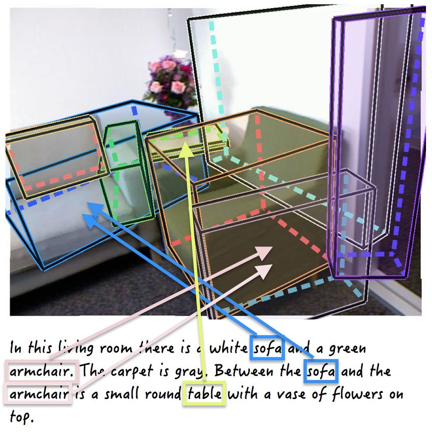
Figure 6. Qualitative results on text to visual object alignment.
                 mantel   count.   toilet   sink   tub    bed    head.   table   shelf   cabin.   sofa   chair   chest   refrig.   oven   micro.   blinds   curtain   board   monit.   print.   avg.
GT        [18]     0.0     83.9     33.3    63.6   12.5   68.6   25.0    50.7    59.5     75.4    54.9   80.2    37.8      7.1      6.5    15.4     63.0     54.7      41.5    31.9     8.0     41.6
cuboids   ours    16.7     84.7     80.0    81.8   33.3   81.7   28.1    66.3    58.6     76.0    61.5   83.2    35.6     35.7      9.7    23.1     64.9     59.7      43.4    58.4    40.0     53.4
our       [18]   100.0     50.3     53.5    45.6   0.0    56.7   34.8    45.4    54.3     50.8    55.6   50.9    50.6     26.1     20.0    45.5     49.5     42.9      47.1    50.0     0.0     44.3
K=8       ours   100.0     52.5     55.1    43.9   0.0    60.3   36.4    51.2    55.4     51.2    55.8   50.3    47.1     38.5      0.0    57.1     52.4     43.6      44.4    61.8    66.7     48.7
our       [18]    50.0     41.2     45.4    43.0   20.0   51.8   30.3    37.5    45.8     43.9    46.5   45.8    38.4     22.7     10.0    40.0     45.9     41.4      39.3    43.9     0.0     37.3
K = 15    ours    50.0     45.7     48.4    42.9   20.0   53.6   32.3    43.0    44.8     45.5    48.8   46.6    36.6     45.8     19.0    51.9     46.6     41.9      51.9    54.9    55.6     44.1
our       [18]     0.0     36.4     44.6    37.0   11.1   46.2   25.5    29.4    39.6     40.0    37.8   40.3    32.5     13.7      7.1    34.3     44.1     38.4      26.1    43.0     0.0     29.9
K = 30    ours    20.0     39.3     47.5    39.4   10.8   48.8   26.7    33.8    39.1     40.4    40.0   41.0    31.7     39.0     13.3    41.0     45.6     38.1      34.3    52.8    34.5     36.1
                   Table 6. Class-wise performance comparison between the baseline (visual only model) and our model.

[21] V. Ordonez, G. Kulkarni, and T. Berg. Im2text: Describ-                                             aligned text corpora. In CVPR, 2010. 2
     ing images using 1 million captioned photographs. In NIPS,                                     [29] N. Srivastava and R. Salakhutdinov. Multimodal learning
     2011. 1, 2                                                                                          with deep boltzmann machines. In NIPS, 2012. 1
[22] A. Quattoni, M. Collins, and T. Darrell. Learning visual rep-                                  [30] V. Stoyanov, N. Gilbert, C. Cardie, and E. Riloff. Conun-
     resentations using images with captions. In CVPR, 2007. 2                                           drums in noun phrase coreference resolution: Making sense
[23] V. Ramanathan, P. Liang, and L. Fei-Fei. Video event under-                                         of the state-of-the-art. In ACL/IJCNLP, 2009. 6
     standing using natural language descriptions. In ICCV, 2013.                                   [31] K. Toutanova, D. Klein, and C. Manning. Feature-rich part-
     2                                                                                                   of-speech tagging with a cyclic dependency network. In
[24] X. Ren, L. Bo, and D. Fox. Rgb-(d) scene labeling: Features                                         HLT-NAACL, 2003. 2, 5
     and algorithms. In CVPR, 2012. 3                                                               [32] M. Vilain, J. Burger, J. Aberdeen, D. Connolly, and
[25] A. Schwing, T. Hazan, M. Pollefeys, and R. Urtasun. Dis-                                            L. Hirschman.       A model-theoretic coreference scoring
     tributed message passing for large scale graphical models. In                                       scheme. In MUC-6, 1995. 6
     CVPR, 2011. 4                                                                                  [33] J. Xiao, J. Hays, K. Ehinger, A. Oliva, and A. Torralba. Sun
[26] A. Schwing, T. Hazan, M. Pollefeys, and R. Urtasun. Effi-                                           database: Large-scale scene recognition from abbey to zoo.
     cient structured prediction with latent variables for general                                       In CVPR, 2010. 3
     graphical models. In ICML, 2012. 4                                                             [34] J. Yao, S. Fidler, and R. Urtasun. Describing the scene as
[27] N. Silberman, P. Kohli, D. Hoiem, and R. Fergus. Indoor                                             a whole: Joint object detection, scene classification and se-
     segmentation and support inference from rgbd images. In                                             mantic segmentation. In CVPR, 2012. 2
     ECCV, 2012. 2, 5                                                                               [35] H. Yu and J. M. Siskind. Grounded language learning from
[28] R. Socher and L. Fei-Fei. Connecting modalities: Semi-                                              video described with sentences. In ACL, 2013. 2
     supervised segmentation and annotation of images using un-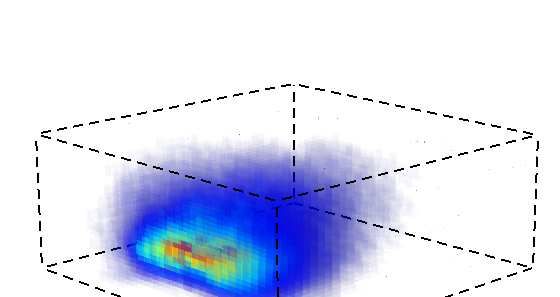
You can also read