A Hybrid Probabilistic Approach for Table Understanding - Jay Pujara
←
→
Page content transcription
If your browser does not render page correctly, please read the page content below
A Hybrid Probabilistic Approach for Table Understanding
Kexuan Sun Harsha Rayudu Jay Pujara
University of Southern California
Information Sciences Institute
kexuansu@usc.edu hrayudu@usc.edu jpujara@isi.edu
Abstract Tables generally contain relational information between
Tables of data are used to record vast amounts of socioeco-
different types of values, such as entities and quantitative
nomic, scientific, and governmental information. Although measurements. To understand a table, an intelligent system
humans create tables using underlying organizational prin- must be able to understand the types of data within a table
ciples, unfortunately AI systems struggle to understand the and the relationships between them. Tables are comprised of
contents of these tables. This paper introduces an end-to-end individual cells which contain a particular type of informa-
system for table understanding, the process of capturing the tion. Cells are spatially organized into regions (or blocks)
relational structure of data in tables. We introduce models that that share a common function. The relationship between
identify cell types, group these cells into blocks of data that the values in a table can be expressed as a relationship be-
serve a similar functional role, and predict the relationships tween these blocks. Our table understanding system adopts
between these blocks. We introduce a hybrid, neuro-symbolic the paradigm of Pujara et al. (2019), which decomposes this
approach, combining embedded representations learned from
thousands of tables with probabilistic constraints that cap-
problem into three tasks: cell classification, block detection,
ture regularities in how humans organize tables. Our neuro- and layout prediction.
symbolic model is better able to capture positional invariants Many prior works have addressed the problems of table
of headers and enforce homogeneity of data types. One lim- understanding in different, piecemeal ways. Traditionally,
itation in this research area is the lack of rich datasets for semantic typing approaches have sought to understand the
evaluating end-to-end table understanding, so we introduce data types within tables, but only operate when data are
a new benchmark dataset comprised of 431 diverse tables organized into well-defined, homogeneous columns. Prior
from data.gov. The evaluation results show that our system
cell classification approaches have focused on identifying
achieves the state-of-the-art performance on cell type classi-
fication, block identification, and relationship prediction, im- functional roles at a cell level rather than capturing broader
proving over prior efforts by up to 7% of macro F1 score. spatial relationships between tabular regions. These meth-
ods range from using handcrafted cell stylistic, format-
ting typographic features (Koci et al. 2016; Chen and Ca-
1 Introduction farella 2013), or embedded vector representations to clas-
Tables are one of the most common ways to organize and sify cells (Ghasemi-Gol, Pujara, and Szekely 2019). Koci
present data. Due to the explosion of information pub- et al. (2019) have investigated finding larger, block struc-
lished on the Web, billions of Web tables (Cafarella et al. tures in tables, however the primary goal of this approach
2008a) covering various topic domains are available. Such is to correct imperfect cell classification results as a post-
tables typically contain valuable information in a richly processing step for cell classification. To our knowledge, the
structured, relational form. Tables include information from task of layout prediction in tables has not been studied in
UN surveys aiding developing nations (Division 2020), ef- prior work, although the broader problem of semantic mod-
forts tracking the spread of pandemics (Atlantic 2020), and eling (Rümmele, Tyshetskiy, and Collins 2018) is an active
the operation of the global economy (Bank 2020). For in- area of research. Our work is the first to combine all three ta-
telligent systems to have meaningful impacts, they must ble understanding tasks in a single, end-to-end system. Fur-
be able to understand the information contained within thermore, our novel neuro-symbolic method is able to cap-
these tables. However, although tables are created follow- ture both stylistic features and statistical patterns of prior ap-
ing established logical structures and topological arrange- proaches, and spatial relationships that encode how humans
ments (Wang 1996), it is difficult for a machine to under- organize tabular data.
stand and extract knowledge from them due to the diversity Despite the availability of vast amounts of tabular data
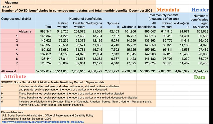
and complexity of their layouts and contents. Figure 1 shows on the Web, annotations for data types, functional regions,
such an example table. It consists of cells with various data and relationships within these tables are very rare. Our ap-
types and functional roles. proach is designed for this environment by combining unsu-
Copyright c 2021, Association for the Advancement of Artificial pervised representation learning and higher-level symbolic
Intelligence (www.aaai.org). All rights reserved. constraints that capture frequent patterns in data. Specifi-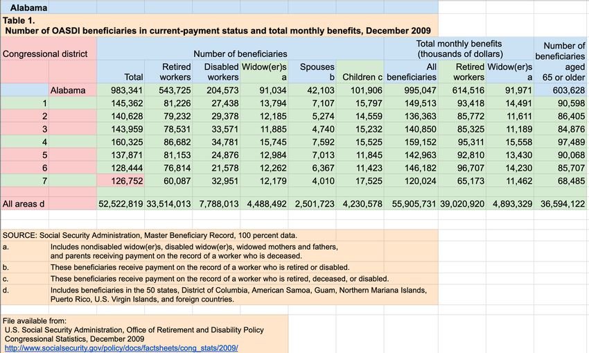
cally, we use high-dimensional table embeddings learned
from thousands of tables in concert with a probabilistic
graphical model, probabilistic soft logic (PSL), that captures
structural patterns, such as consistency of types among con-
tiguous cells. Together, these two techniques are capable of
harnessing vast amounts of data while explicitly incorporat-
ing the intuitions human use when constructing tables.
   Since previous work does not have a rich enough learning
resource that covers all aspects of these tasks, we introduce
a new benchmark dataset comprised of 431 tables down-
loaded from the U.S. Government’s open data (Data.gov
2019). These tables are in different formats such as spread-
                                                                   Figure 1: An example table with colored regions of cells.
sheets and comma-separated values, and from various
topic domains. Most existing benchmark datasets (such as
DeEx (DeEx 2013), SAUS (SAUS 2014) and CIUS (CIUS
2019)) consist of only Excel files, are from narrow domains       2.2   Cell Embeddings
and cover only cell functional types. Cross validation shows      Cell embeddings are vector representations of tabular cells.
that the proposed system outperforms other baseline ap-           Ghasemi-Gol, Pujara, and Szekely (2019) proposed to use
proaches in most cases. The results align with our hypothe-       neural networks to learn the cell embeddings. Each embed-
ses: the pre-trained cell embeddings encapsulate useful in-       ding consists of two parts, i.e. the contextual embedding cap-
formation of cells and probabilistic constraints can help en-     tures the semantic information of the cell content, and the
force the logical consistency of prediction. Accordingly, the     stylistic embedding encapsulates the stylistic features of the
neuro-symbolic approach gets the best of both worlds. The         cell. There are different ways to capture the contextual and
idea of neuro-symbolic combination could potentially be ap-       stylistic information. Specifically, the authors exploit pre-
plied to investigate other tasks for tables such as data trans-   trained language models to identify the local context of cells
formation and relation extraction. In addition, the blocks and    and auto-encoders to encode the stylistic features. Accord-
the relationships extracted by our system could potentially       ingly, in our system, we use their pre-trained cell embedding
be used for automated tabular analysis such as finding im-        model learned from thousands of tables.
portant patterns from a table (Zhou et al. 2020).
   We summarize our primary contributions:                                        3    Problem Definition
• An integrated system solves three table understanding           In this section, we reformalize tabular data and three table
  tasks inspired by human organization of tables: cell clas-      understanding tasks introduced in (Pujara et al. 2019). A ta-
  sification, block detection and layout prediction.              ble is a matrix T = {vi,j |1 ≤ i ≤ N, 1 ≤ j ≤ M } where
• A hybrid neuro-symbolic approach leveraging the                 N is the number of rows, M is the number of columns, and
  strength of embedded cell representations with constraints      vi,j is the cell in the ith row and the j th column.
  capturing human layout patterns.
• A new and richer benchmark dataset with annotations for         3.1   Cell Classification
  three tasks to support ongoing research in table under-         The goal of cell classification is to assign a label to each
  standing.                                                       cell. In most prior work, cell classification is to assign each
                                                                  cell a label indicating the functional role the cell presents in
                    2   Preliminaries                             the data layout. This process should consider both the cell
2.1   PSL                                                         information and context information of neighboring cells or
                                                                  even the whole table. In this paper, we classify cells only
Probabilistic Soft Logic (Bach et al. 2017) is a probabilistic    based on cell contents without considering the contextual
inference framework. A PSL model is defined on a set of           information. We leave the task of identifying cell functional
predicates and a set of first-order logic rules consisting of     roles to the block detection task.
the predicates. Here is an example PSL rule:                         There are different ways to classify cell contents. Since
         w : P 1(X, Y ) ∧ P 2(X, Z) ⇒ P 3(Y, Z)                   the content usually is a sequence of characters, the most ba-
                                                                  sic types can be Number, String, Datetime and Empty. How-
where w is the weight of this rule, P 1, P 2 and P 3 are three    ever, these types are not informative enough. For example,
predicates, and X, Y and Z are variables. During inference,       knowing a cell contains a string is not helpful enough for un-
the variables are grounded by constants. PSL uses hinge-          derstanding the table. In this paper, we use more fine-grained
loss Markov Random Fields (MRFs) to efficiently solve the         semantic data types. A number can be a Nominal, Cardinal
convex optimization problem.                                      or Ordinal, and a string can be the name of a Person, an Or-
   PSL has been successfully applied to solve different tasks     ganization, a Location, or Other string. Particularly, this task
such as knowledge base completion (Chen et al. 2019), rec-        can be even challenging for human. For example, a zip code
ommender systems (Kouki et al. 2015), and entity resolu-          is a Nominal but can be easily identified as a Cardinal, and
tion (Kouki et al. 2017).                                         a year is a Datetime but can also be classified as a Cardinal .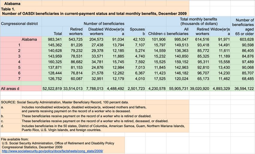
4.1     Cell Classifier
                                                                   The cell classifier operates in two processes. In training
                                                                   phase, a statistical learning model learns to predict a can-
                                                                   didate data type using cell embeddings. In inference phase,
                                                                   a PSL model enforces constraints between the data types.
                                                                      To model this task, we first identify several simple fea-
             Figure 2: Our system architecture.                    tures based on cell content, such as IsNumber, IsDate
                                                                   and IsEmpty, indicating if the content could be parsed as
                                                                   a number, a date/time, or other special cases such as empty
3.2   Block Detection                                              cells or reserved values such as “n/a”, respectively. We then
The goal of block detection is to identify regions of cells        extract dependencies between the features and data types.
playing the same functional role. We refer to each such a re-      The PSL model consists of a set of rules presenting such de-
gion as a block. We define a block as a rectangle denoted as       pendencies. In our model, we are interested in predicting the
hT, L, B, Ri where the four indices represent the Top row,         cell data types (DataType). Some example rules are:
Left column, Bottom row and Right column of the block, re-                     IsDate(C) ⇒ DataType(C, “datetime”)
spectively. The smallest block is a single cell and the largest             CELabel(C, T ) ⇒ DataType(C, T )
block is the table itself. When we treat each cell as a block,
the system eventually solves the cell functional type classi-
fication. However, our goal is to identify regions as large as        The first rule expresses: if the cell content C is success-
possible such that cells in the same region indeed play the        fully parsed as a datetime, we could confidently label it as
same functional role. As shown in (Koci et al. 2019), con-         “Datetime”. CELabel shows the candidate data type pre-
sidering blocks rather than individual cells could potentially     dicted by the statistical learning model.
reduce the number of misclassifications.                              The above implication rules are introduced to avoid cell
   We consider the following functional roles: Metadata de-        embeddings being overfitted and making mistakes in obvi-
                                                                   ous situations. However, the above rules are not always suf-
notes the global information of the table (such as the ti-         ficient to differentiate data types from each other, especially
tle and source); Header indicates attribute names of the ta-       for numbers. For example, “2020” could be a number indi-
ble columns; Attribute presents attribute names of the table       cating a quantity or a specific year. To alleviate this issue,
rows; and Data shows the main content of the table.                we also introduce several conjunctive rules. For example:
3.3   Layout Prediction                                                    IsNum(C)∧! IsInt(C) ⇒ DataType(C, “cardinal00 )
Given the blocks identified from the previous task, the goal       HasAlpha(C)∧! HasNum(C) ⇒! DataType(C, “cardinal00 )
of layout prediction is to determine the relationships be-               OneWord(C) ∧ HasNum(C) ⇒! DataType(C, “person00 )
tween blocks. Each pair of blocks will be assigned a rela-
tionship. We consider the following four relationships: Sub-
set of denotes that a block shows the subcategory infor-              These rules are derived from constraints upon how hu-
mation of another block (usually between two Header or             mans express different types of cell content. The first two
Attribute blocks); Header of indicates a block to contain          rules demonstrate how numbers exist in tables. Usually,
the header information of another block (usually between           floating (not integer) numbers are only used to show quanti-
a Header and a Data block); Attribute of marks a block to          ties, such as average numbers of people and average scores
record the attribute information of another block (usually be-     of classes, which are cardinals. In addition, cardinals always
tween an Attribute and a Data block); and Global Attribute         contain some numeric characters. The third rule shows a per-
marks a block containing the global information of another         son’s name usually is not a single token with numeric values.
block (usually between a Metadata block and another block).        We note that the above rules are only a subset of rules used
                                                                   in the system. We provide the full list of rules in Appendix.
                        4    Method                                4.2     Block Detector
We introduce our system for table understanding, illustrated
                                                                   The block detector takes the cell data types and cell embed-
in Figure 2. In specific, the system takes a table as the in-
                                                                   dings as inputs to identify blocks, and assign each block
put and uses a pre-trained cell embedding model to repre-
                                                                   a functional label. This component operates in three steps:
sent each cell that is to be processed by several downstream
                                                                   generating candidate blocks, enforcing probabilistic con-
predictors. More specifically, the cell classifier seeks to pre-
                                                                   straints, and coalescing blocks.
dict cell data types and the block detector uses both the em-
beddings and the data types to generate blocks. The layout         Generating Candidate Blocks Different from the region-
predictor then predicts relationships between blocks. The          based approach (Koci et al. 2019) that groups adjacent cells
cell classifier, block extractor and layout predictor model the    into rectangular regions, we introduce a top-down approach.
three corresponding tasks as PSL problems. Our system de-          It starts from a whole table and recursively splits the table
pends on the computational performance of PSL. Empiri-             into smaller blocks. This idea is inspired by the Bayesian
cally, the inference of PSL scales linearly with the number        CART model which constructs a decision tree by recursively
of potentials and constraints (Bach et al. 2017) which is at       partitioning a space into subsets (Chipman, George, and Mc-
most linear to the number of cells in our problem.                 Culloch 1998). Figure 3 demonstrates such a decision tree.
Algorithm 1: Candidate Block Generation
1 Function Split(block):
2 queue ←− {(block, 0)}; blocks ←− {};
3 while queue 6= ∅ do
4 (ht, b, l, ri , d) ←− queue.get()
// t, b, l, and r are indices.
5 Randomly select a number v within [0, 1]
Figure 3: An illustration of block generation. T is the orig- 6 if v < psplit (d) then
inal table, B1, B2, B3 and B4 are non-overlapping blocks 7 Randomly split ht, b, l, ri into B1 and B2
in the table (left) and leaf nodes in the decision tree (right). using prule .
8 queue.push((B1 , d + 1))
9 queue.push((B2 , d + 1))
10 else
Instead of constructing the tree greedily, Chipman et 11 blocks.add(ht, b, l, ri)
al. introduced a Markov Chain Monte-Carlo (MCMC) ap-
12 return blocks;
proach to finding the tree. Formally, we start from the table
T , at each step i, for each active node Bij , we choose to 13 Function GenerateATree(T , types):
either split this node into two children nodes or stop at this 14 row blocks = Split(T ); // Row-wise
node with the splitting probability psplit . If a node is cho- 15 blocks ←− ∅;
16 foreach B in row blocks do
sen to be split, we select the row/column to split following 17 blocks.union(Split(B)) // Column-wise
the rule distribution prule , otherwise we stop splitting this
node and it becomes a leaf node. For example, in fig. 3, T 18 return blocks;
is split into B1 and another node. B1 is not split so it be- 19 Function SampleATree(T , types, N ):
comes a leaf node while the other node is further split into 20 trees ←− ∅
two extra nodes. Each leaf node becomes a candidate block 21 foreach 1 ≤ i ≤ N do
in our problem. Following this process, the system generates 22 trees.add(GenerateATree(T, types))
N such trees and randomly select one tree, with the weight 23 return Sample a tree from trees using Went .
function Went , to finalize candidate blocks.
Algorithm 1 shows the details. We call the function
SampleATree to generate candidate blocks. Similar to the
Bayesian CART model, we set the splitting probability to be
1
psplit (d) = (1+d) β where β is a hyperparameter and d is the CELabel(B, L) ⇒ BT(B, L)
depth of the node. A larger β indicates a smaller tree. FirstRow(B) ⇒ BT(B, ”header”)
We make use of the cell data types provided by the cell
classifier to decide the rule distribution. At node Bi , sup- BT(B, L) indicates the possibility that block B is as-
pose it can be split into two children nodes Bi1 and Bi2 , signed label L. Same as the cell classifier, CELabel shows
the1 data type distributions
of Bi1 and Bi2 are Di1 = how the block detector uses cell embeddings. The statistical
d1 , d12 , · · · , d1k and Di2 = d21 , d22 , · · · , d2k where k is learning model assigns each cell a label. Since a block may
the number of data types. We set the rule distribution to be have more than one cell, CELabel(B, L) reveals the possi-
λ
− 2
prule (Bi1 , Bi2 ) = λ · e |Di1 −Di2 |2 where λ is a hyperpa- bility that block B is assigned label L. This corresponds to
rameter. This is designed based on the assumption that a split the ratio of the number of cells assigned label L over the to-
which makes the distributions more diverse is more likely to tal number of cells in B. The second rule expresses: blocks
be chosen. We apply the exponential family λ · e−λ to make on the first row usually is a Header block.
the difference between the distributions more significant. In addition to the simple rules listed above, we also ap-
We use the entropy Went to determine the weight of a ply several conjunctive rules that fuse the inherent positional
− λ ! constraints within the table layouts. For example:
P |b| P t t
−P t p log p
b:B b|b0 |
b
tree. Went (B) = λ · e b0 :B where B
is a set of blocks , b is a block, |b| is the size (area) of b, and SameRow(B1 , B2 ) ∧ BT(B1 , ”header”) ⇒ BT(B2 , ”header”)
ptb is the ratio of the cells with the data type t in b. The λ Abv(B1 , B2 ) ∧ Abv(B2 , B3 ) ∧ BT(B1 , C) ∧ BT(B3 , C)
here is the same as the λ in prule . ⇒ BT(B2 , C)
Enforcing Probabilistic Constraints In the second step, The first rule indicates that if a block is a Header block,
we assign a functional label to each candidate block using a blocks that on the same row as this block are also Header
PSL model. Same as the cell classifier, we perform this step blocks. The last rule takes neighboring blocks into consider-
with two components: a statistical learning model that takes ation. If the neighbor above and the below it have the same
a cell embedding as an input to predict a functional label label, it should also be assigned this label. These conjunctive
for each cell, and a PSL model that enforces probabilistic constraints exploit the power of collective classification that
constraints. A set of example rules are listed below: probabilistic models perform.Block Coalescing After assigning labels to the candidate three tasks. The results are 0.937 for cell classification, 0.960
blocks, we apply a post-processing step to merge small for block deteection, and 0.936 for layout prediction, which
blocks into large blocks. In this step, we first merge neigh- indicate the good reliability of the annotations. Specifically,
boring blocks if they have the same top row, bottom row for block detection, we align the blocks from annotator A
and labels. Similarly, we then merge neighboring blocks if with those from annotator B and then compare the labels.
they have the same left column, right column and labels. The
block detector finally passes the merged blocks to the layout
predictor. We design this step to resolve the issue of over-
6 Evaluation
partitioning and produce better blocks. In this section, we present the experimental evaluation of
the proposed system based on the four datasets. In the pro-
4.3 Layout Predictor cess of creating PSL rules, we randomly selected 10 tables
The layout predictor is the last component of our system. It from each dataset as a rule development set. These tables
predicts a relationship between each pair of blocks identified are not included in any training and testing. In all experi-
by the block detector. We model the task as a PSL problem ments, we perform 5-fold cross validation on the rest of the
utilizing relative positional relationships between the blocks. tables: for each dataset, we randomly split the tables into
A set of example rules are listed below: 5 folds, train/validate a model using 4 folds and test on 1
fold. For the 4 folds, we randomly split the tables with 9:1
Adj(B1 , B2 ) ∧ BT(B1 , ”data”) ∧ BT(B2 , ”data”) ratio into training and validation sets. The results are aver-
aged on the 5 test folds. Each cell embedding consists of
⇒ Rel(B1 , B2 , ”empty”)
40-dimensional stylistic features and 512-dimensional con-
Hrz(B1 , B2 ) ∧ BT(B1 , ”attr”) ∧ BT(B2 , ”data”) textual embedding.
⇒ Rel(B1 , B2 , ”attribute”)
6.1 Cell Classification
These rules illustrate our hypotheses about positional re-
lationships between blocks. If two data blocks are neighbors, As described in Section 3.1, we evaluate our cell classifier
they might not have any special relationship. If two blocks on the DG dataset. Each cell is classified into 1 of the 9
are horizontally aligned, one is an attribute block and the data types: empty (Emp), cardinal (Card), Nominal (Nom),
other one is a data block, the attribute block might reveal ordinal (Ord), datetime (Date), location (Loc), organiza-
attributes of the data within the data block. tion (Org), person (Per), and other string (Str). In the PSL
model, we leverage 32 logical rules.
5 Datasets for Table Understanding We compare our system with the following baselines:
1) Random Forest (RF): We use the RandomForest clas-
5.1 Existing Datasets sifier in scikit-learn library (Buitinck et al. 2013). It
There are three main datasets DeEx, CIUS and SAUS de- takes cell embeddings as input the predict a cell data
signed for evaluating cell functional type classification. type. We select n estimator among [100, 300], max depth
The DeEx dataset was collected in the DeExcelerator among [5, 50, N one], min sample split among [2, 10] and
project (Eberius et al. 2013) and contains 457 annotated min samples leaf among [1, 10]. We use the bootstrap mode
sheets. The CIUS dataset was originally from the Crime In with balanced sub-sampling. 2) Conditional Random Field
the US (CIUS) database and contains 268 sheets. The SAUS (CRF): CRFs are a type of PGMs, which takes the con-
dataset was downloaded from the U.S. Census Burea (Chen text (neighboring cells in tabular data) into consideration. In
and Cafarella 2014) and contains 210 sheets. Both the CIUS this experiment, it uses a feature set introduced in in (Chen
and SAUS datasets were annotated by Ghasemi-Gol, Pujara, and Cafarella 2013) to make predictions. We choose 2-
and Szekely (2019). We evaluate our approach on all these dimensional CRF to represent row-wise and column-wise
three datasets for the task of block detection. These three neighborhood interactions. We use GridCRF class from
datasets are cell-level annotations based on functional roles. the pystruct library (Müller and Behnke 2014). We set the
max iter to be 500, tolerance to be 0.01 and select c range
5.2 A New Dataset from Data.gov among [0.01, 0.1, 1.0]. 3) Multi-layer Perceptron (MLP)
The existing datasets, designed for evaluating cell functional We use the pytorch library (Paszke et al. 2019) to create a
type classification, have relatively narrow domains and fo- two-layer neural network with the Rectified Linear activa-
cus only on Excel files. To evaluate the three aforementioned tion function (ReLU). It also takes cell embeddings as input.
table understanding tasks, we introduce a new dataset DG. We set batch size to be 32, learning rate to be 0.0001, and
We downloaded 1837 files from the U.S. Open Data website epoch to be 50. We use cross entropy loss.
(data.gov). These files are from different topic domains such Results: Table 1 shows the results of this experiment. For
as agriculture, climate, ocean and ecosystem, and are in dif- both RF and MLP, the PSL model improves over their re-
ferent formats (i.e. csv and Excel). We sampled 431 tables sults. The results demonstrate that the logical rules are able
from these files and annotated them for the three table un- to provide useful high-level constraints between data types
derstanding tasks. To show inter-annotator agreements, we and cell-level features. Compared to CRF, it is more flexi-
ask two annotators to independently annotate 25 tables and ble to enforce explicit constraints in PSL. For each table, the
evaluate the Cohen’s kappa coefficients (McHugh 2012) for average running time of PSL is 10 seconds.Table 1: Data type classification results (F1 scores) on DG. Table 2: Results of block detection models.
Avg is the macro F1 score (%) ± the standard deviation.
(a) Cell functional type classification results. The annotations are
Emp Crd Str Dat Loc Org Ord Nom Per Avg same as those in table 1. All models use the outputs of the PSL
(RF) cell classifier.
CRF 81.9 82.5 42.4 56.2 34.4 16.8 0.0 36.0 1.3 39.1±1.8
MLP 84.5 85.6 69.1 59.3 54.9 46.8 0.0 52.0 1.2 50.4±5.4
RF 85.0 84.4 73.2 61.4 65.2 55.5 0.3 53.4 39.3 57.5±4.7 MD DT HD AT Avg
PSL 96.5 88.3 70.2 77.8 55.8 43.3 0.3 52.4 1.0 54.0±3.1
(MLP) CRF 96.5 67.6 94.9 36.8 73.9±8.9
PSL 96.8 87.8 74.3 78.4 66.1 52.5 0.2 53.0 31.7 60.1±3.2
RNN 99.5 99.3 97.4 90.5 96.7±4.1
CIUS
(RF)
RF 95.9 99.7 88.9 97.0 95.4±0.6
PSL(RNN) 94.8 99.2 97.8 89.3 95.3±4.1
PSL(RF) 93.6 99.7 96.0 97.6 96.7±1.1
6.2 Block Detection
We use 19 rules in the PSL model with the same weight. We CRF 80.7 82.2 95.7 38.2 74.2±5.8
RNN 94.3 97.5 84.1 79.5 88.9±2.3
SAUS
conduct two experiments. First, since the existing datasets
are for cell role type classification, however, our system RF 79.1 98.6 78.8 91.1 86.9±4.0
identifies block role type. To compare with baseline mod- PSL(RNN) 87.6 97.8 86.7 79.5 87.9±1.4
els on these datasets, we assign each cell a functional role PSL(RF) 80.6 99.0 85.4 92.8 89.4±2.5
according to the predictions for blocks. Second, we mea- CRF 35.6 55.7 48.0 1.7 35.3±6.9
sure how precisely predicted blocks are aligned with ground- RNN 33.8 96.1 47.2 39.5 54.2±5.9
DeEx
truth blocks. We borrow the idea of Error-of-Boundary RF 53.4 98.4 51.0 26.5 57.3±2.0
(EoB) proposed in Dong et al. (2019): PSL(RNN) 38.5 97.2 53.5 44.9 58.5±8.0
PSL(RF) 65.4 98.8 60.5 26.0 62.7±3.9
EoB(B gt , B p ) =
CRF 41.3 53.1 94.1 34.8 55.9±9.3
max |Btgt − Btp |, |Bbgt − Bbp |, |Blgt − Blp |, |Brgt − Brp |
DG RNN 45.4 95.9 82.9 78.8 75.8±4.3
where Btgt , Bbgt , Blgt , and Brgt are the top row, bottom row, RF 74.0 95.8 80.7 77.8 82.1±2.5
left column, and right column of the ground-truth block B gt . PSL(RNN) 69.9 95.7 89.2 77.4 83.1±5.2
The annotations are same for the predicted block B p . Since a PSL(RF) 77.2 95.7 91.4 77.4 85.4±4.8
table may have several blocks, instead of evaluating a single (b) Average EoB scores of all models on the DG dataset.
block, we use averaged EoB over all blocks:
Method CRF RNN RF PSL (RNN) PSL (RF)
X 1 ij ij
EoBavg 5179 24192 59403 2828 1995
EoBavg = EoB(B gt , B p )
1≤i≤N,1≤j≤M
|B gtij ∩ B pij |
where N is the number of rows, M is the number of
ij
columns, B gt is the block that the cell on the ith row and It is the classification model proposed in (Ghasemi-Gol, Pu-
ij jara, and Szekely 2019). We set the epoch to be 50 and learn-
j th column belongs to. Same for B p .
ing rate to be 0.0001. In the second experiment, we use the
In the system, we set the number of sample trees to
region-based approach from (Koci et al. 2019) to create
be 50, select the α among [0.01, 0.05, ] and λ among
blocks: it builds row-label intervals (RLI) (i.e. neighboring
[5, 10]. Following (Ghasemi-Gol, Pujara, and Szekely 2019),
cells with the same label on the same row), and then merge
we compare the system with the following baselines: 1)
RLIs in adjacent rows into regions.
Random Forest (RF): In the first experiment, it takes
cell embeddings as input to predict a role type for each Results Table 2a shows the results of the first experiment.
cell. We also use the RandomForest class from scikit- The PSL model improves the performance over baseline
learn. We select n estimator among [100, 300], max depth classifiers (i.e. RF and RNN) using cell embeddings. The
among [5, 50, N one], min sample split among [2, 10] and reasons are: 1) the rectangular block representations guar-
min samples leaf among [1, 10]. We use the bootstrap mode antee the cells within a block have the same type, and 2)
with balanced sub-sampling. 2) Conditional Random Field the explicit constraints between positional features and the
(CRF): We follow the instructions in (Chen and Cafarella functional types, and between the functional types them-
2013) to implement the linear CRF. We use the ChainCRF selves further assist the performance. The major challenge
class from the pystruct library. We set max iter to be 1000, that PSL leads to lower accuracy in some cases (such as MD
tol to be 0.01, and select C range from [0.1, 0.3, 0.5, 0.7, in DeEx and AT in DG) is that the method uses data type
1.0]. We use the same feature set as is used in the CRF distributions to decide the division of a block. If two adja-
model in the previous experiment. The CRF takes the inter- cent rows/columns have very similar data type distributions,
dependencies between rows and predict the functional type they are less likely to be split.
(only metadata, data and header) of each row. For data rows, Table 2b presents the results of the second experiment. In
cells with actual numbers are classified as data and other terms of the average EoB, our model shows better results.
cells are attributes. 3) Recurrent Neural Network (RNN): We present the results of the example table of Figure 1 inTable 3: Layout prediction results on the DG dataset. All
models use the outputs of the PSL (F) block detector.
Method EP HO AO GA SC Avg
RF 81.7 1.1 2.1 22.7 0.0 21.5±1.2
CRF 88.5 33.7 32.2 40.0 0.0 38.9±3.1
PSL 89.6 70.3 32.8 43.0 25.6 52.3±3.4
to run different layout prediction methods. For each block b,
we match it with the ground-truth block b0 which shares the
most overlapping cells with b. All predicted relationships for
(a) The result of the RF model (using cell embeddings only).
b are added to b0 and compared with the ground-truth rela-
tionships. Table 3 shows the results. The PSL model per-
forms better than the compared models in most cases. For
each table, the average running time of PSL is 0.4 seconds.
7 Related Work
In recent years, a large amount of research efforts seek to
solve different tasks for automated processing tabular data,
such as table detection, table classification, and data trans-
formation. Wang and Hu (2002); Wang et al. (2012); Fang
et al. (2012) focus on extracting tables from HTML pages,
document images and PDFs, and Dong et al. (2019) lever-
ages the convolutional neural networks (CNN) to develop an
(b) The result of the PSL model.
end-to-end framework for spreadsheet table detection. Ca-
Figure 4: The block detection results of the table in Figure 1. farella et al. (2008b), Crestan and Pantel (2010) and Eberius
et al. (2015) introduced content, lexical, global and local
features, and Nishida et al. (2017) proposed a hybrid ar-
chitecture TabNet using recurrent neural networks and CNN
Figure 4 to demonstrate the reason. The RF (similar for CRF to encode tabular data, to perform table type classification.
and RNN) model depends only on the cell classification re- The task of tabular data transformation is transform tabu-
sults so that the misclassified cells scattered over the whole lar data into more formal tables, i.e. relational databases. Su
table make the generated blocks small and affect the EoB. et al. (2017); Shigarov et al. (2016); Dou et al. (2018) used
For a table in CIUS, SAUS, DeEx, and DG, the average run- either engineered or automatically inferred features to con-
ning times of PSL are 39, 3, 17, and 7 seconds, respectively. struct rule-based engines.
6.3 Layout Prediction 8 Conclusions and Future Work
We use 15 logical rules in the system. We evaluate the per- In this paper, we proposed an end-to-end system for solv-
formance of the layout predictor on the DG dataset. We use 5 ing three table understanding tasks, i.e. cell classification,
aforementioned relationships: empty (EP), header of (HO), block detection and layout prediction. Our system exploits
attribute of (AO), global attribute (GA) and supercategory the rich information within cell embeddings as well as logi-
of (SC). We compare the predictor with the following two cal constraints following the principles of the layouts of the
baselines: 1) Random Forest (RF): For every two blocks, tabular data. We introduced probabilistic rules and used the
we use a few manually crafted features: their functional la- probabilistic inference framework PSL to enforce the rules.
bels (predicted by the block detector), and several relation- We experimentally evaluated our system and showed the re-
ships between blocks ( below, above, left right, adjacent, and sults. The output of our system can potentially be used for
overlap). We use the RandomForest from the scikit-learn li- solving several downstream tasks such as semantic model-
brary. We select n estimators among [100, 300], max depth ing, table summarization, and question answering on tables.
among [5, 50, None], min samples split among [2, 10] and For example, in semantic modeling, each identified block
min samples leaf among [1, 10]. 2) Conditional Random can be treated as an attribute and the relationships between
Field (CRF) We construct a graph CRF for this task. If we blocks are helpful for predicting better semantic models.
treat each block as a node and the relationship between two In the current system, we use the distributions of cell data
blocks as an edge, the above features are features associ- types to generate candidate blocks. Alternative measures and
ated with edges. We use the EdgeFeatureGraphCRF from sampling strategies could also be leveraged. In addition, the
the pystruct library. We set max iter to be 50, tol to be 0.01, idea of combining embeddings and probabilistic constraints
and select C range among [0.01, 0.1], could potentially be used for solving the layout prediction
Results We use the blocks generated by the block detector and other tasks related to tables.9 Acknowledgements Dou, W.; Han, S.; Xu, L.; Zhang, D.; and Wei, J. 2018. Expand-
We thank Majid Ghasemi Gol for his kind help at the be- able Group Identification in Spreadsheets. In Proceedings of the
33rd ACM/IEEE International Conference on Automated Software
ginning of the project, and Muhao Chen for his excellent
Engineering, ASE 2018, 498–508. ISBN 9781450359375. doi:
feedback and advice for the paper. We also thank anony- 10.1145/3238147.3238222.
mous reviewers for their valuable comments and sugges-
tions. This research is supported by the Defense Advanced Eberius, J.; Braunschweig, K.; Hentsch, M.; Thiele, M.; Ahmadov,
Research Projects Agency (DARPA) and the Air Force Re- A.; and Lehner, W. 2015. Building the Dresden Web Table Corpus:
A Classification Approach. In 2015 IEEE/ACM 2nd International
search Laboratory (AFRL) under contracts FA8650-17-C- Symposium on Big Data Computing (BDC), 41–50.
7715 and FA8750-17-C-0106.
Eberius, J.; Werner, C.; Thiele, M.; Braunschweig, K.; Dannecker,
References L.; and Lehner, W. 2013. DeExcelerator: a framework for extract-
ing relational data from partially structured documents. In Proceed-
Atlantic, T. 2020. Covid Tracking Data. https://covidtracking.com/ ings of the 22nd ACM international conference on Information &
data/national/cases. Knowledge Management, 2477–2480.
Bach, S. H.; Broecheler, M.; Huang, B.; and Getoor, L. 2017. Fang, J.; Mitra, P.; Tang, Z.; and Giles, C. L. 2012. Table Header
Hinge-Loss Markov Random Fields and Probabilistic Soft Logic Detection and Classification. In AAAI.
18(1): 3846–3912. ISSN 1532-4435.
Ghasemi-Gol, M.; Pujara, J.; and Szekely, P. 2019. Tabular Cell
Bank, T. W. 2020. Global economic perspectives. https://www.
Classification Using Pre-Trained Cell Embeddings. In Interna-
worldbank.org/en/publication/global-economic-prospects.
tional Conference on Data Mining.
Buitinck, L.; Louppe, G.; Blondel, M.; Pedregosa, F.; Mueller, A.;
Koci, E.; Thiele, M.; Romero, O.; and Lehner, W. 2016. A Ma-
Grisel, O.; Niculae, V.; Prettenhofer, P.; Gramfort, A.; Grobler, J.;
chine Learning Approach for Layout Inference in Spreadsheets. In
Layton, R.; VanderPlas, J.; Joly, A.; Holt, B.; and Varoquaux, G.
Proceedings of the International Joint Conference on Knowledge
2013. API design for machine learning software: experiences from
Discovery, Knowledge Engineering and Knowledge Management,
the scikit-learn project. In ECML PKDD Workshop: Languages for
77–88. ISBN 9789897582035.
Data Mining and Machine Learning, 108–122.
Cafarella, M. J.; Halevy, A.; Wang, D. Z.; Wu, E.; and Zhang, Koci, E.; Thiele, M.; Romero, O.; and Lehner, W. 2019. Cell Clas-
Y. 2008a. WebTables: Exploring the Power of Tables on the sification for Layout Recognition in Spreadsheets. In Knowledge
Web. Proc. VLDB Endow. 1(1): 538–549. ISSN 2150-8097. doi: Discovery, Knowledge Engineering and Knowledge Management,
10.14778/1453856.1453916. 78–100. Cham: Springer International Publishing.
Cafarella, M. J.; Halevy, A.; Wang, D. Z.; Wu, E.; and Zhang, Kouki, P.; Fakhraei, S.; Foulds, J.; Eirinaki, M.; and Getoor, L.
Y. 2008b. WebTables: Exploring the Power of Tables on the 2015. HyPER: A Flexible and Extensible Probabilistic Frame-
Web. Proc. VLDB Endow. 1(1): 538–549. ISSN 2150-8097. doi: work for Hybrid Recommender Systems. In Proceedings of the
10.14778/1453856.1453916. 9th ACM Conference on Recommender Systems, 99–106. ISBN
9781450336925. doi:10.1145/2792838.2800175.
Chen, X.; Chen, M.; Shi, W.; Sun, Y.; and Zaniolo, C. 2019. Em-
bedding Uncertain Knowledge Graph. In AAAI. Kouki, P.; Pujara, J.; Marcum, C.; Koehly, L.; and Getoor, L. 2017.
Collective Entity Resolution in Familial Networks. In IEEE Inter-
Chen, Z.; and Cafarella, M. 2013. Automatic Web Spreadsheet national Conference on Data Mining.
Data Extraction. In Proceedings of the 3rd International Workshop
on Semantic Search Over the Web. ISBN 9781450324830. McHugh, M. 2012. Interrater reliability: The kappa statis-
tic. Biochemia medica : časopis Hrvatskoga društva medicinskih
Chen, Z.; and Cafarella, M. 2014. Integrating Spreadsheet Data via biokemičara / HDMB 22: 276–82. doi:10.11613/BM.2012.031.
Accurate and Low-Effort Extraction. In Proceedings of the 20th
ACM SIGKDD International Conference on Knowledge Discovery Müller, A. C.; and Behnke, S. 2014. PyStruct: Learning Struc-
and Data Mining, 1126–1135. ISBN 9781450329569. tured Prediction in Python. J. Mach. Learn. Res. 15(1): 2055–2060.
ISSN 1532-4435.
Chipman, H. A.; George, E. I.; and McCulloch, R. E. 1998.
Bayesian CART Model Search. Journal of the American Statis- Nishida, K.; Sadamitsu, K.; Higashinaka, R.; and Matsuo, Y.
tical Association 93(443): 935–948. doi:10.1080/01621459.1998. 2017. Understanding the Semantic Structures of Tables with a Hy-
10473750. brid Deep Neural Network Architecture. In Proceedings of the
Thirty-First AAAI Conference on Artificial Intelligence, AAAI’17,
CIUS. 2019. CIUS. https://ucr.fbi.gov/crime-in-the-u.s.
168–174.
Crestan, E.; and Pantel, P. 2010. A Fine-Grained Taxonomy of
Tables on the Web. In Proceedings of the 19th ACM International Paszke, A.; Gross, S.; Massa, F.; Lerer, A.; Bradbury, J.; Chanan,
Conference on Information and Knowledge Management, CIKM G.; Killeen, T.; Lin, Z.; Gimelshein, N.; Antiga, L.; Desmaison,
’10, 1405–1408. ISBN 9781450300995. doi:10.1145/1871437. A.; Kopf, A.; Yang, E.; DeVito, Z.; Raison, M.; Tejani, A.; Chil-
1871633. amkurthy, S.; Steiner, B.; Fang, L.; Bai, J.; and Chintala, S. 2019.
PyTorch: An Imperative Style, High-Performance Deep Learning
Data.gov. 2019. Data.gov. https://www.data.gov/. Library. In Advances in Neural Information Processing Systems
DeEx. 2013. DeExcelarator. https://wwwdb.inf.tu-dresden.de/ 32, 8024–8035.
research-projects/deexcelarator/. Pujara, J.; Rajendran, A.; Ghasemi-Gol, M.; and Szekely, P. 2019.
Division, U. N. S. 2020. UNdata. http://data.un.org/. A Common Framework for Developing Table Understanding Mod-
Dong, H.; Liu, S.; Han, S.; Fu, Z.; and Zhang, D. 2019. TableSense: els. In International Semantic Web Conference - Posters.
Spreadsheet Table Detection with Convolutional Neural Networks. Rümmele, N.; Tyshetskiy, Y.; and Collins, A. 2018. Evaluating ap-
In AAAI. proaches for supervised semantic labeling. CoRR abs/1801.09788.SAUS. 2014. SAUS. http://dbgroup.eecs.umich.edu/project/sheets/ datasets.htm. Shigarov, A. O.; Paramonov, V. V.; Belykh, P. V.; and Bondarev, A. I. 2016. Rule-Based Canonicalization of Arbitrary Tables in Spreadsheets. In Dregvaite, G.; and Damasevicius, R., eds., Infor- mation and Software Technologies, 78–91. Cham: Springer Inter- national Publishing. ISBN 978-3-319-46254-7. Su, H.; Li, Y.; Wang, X.; Hao, G.; Lai, Y.; and Wang, W. 2017. Transforming a Nonstandard Table into Formalized Tables. 311– 316. doi:10.1109/WISA.2017.38. Wang, J.; Wang, H.; Wang, Z.; and Zhu, K. Q. 2012. Understand- ing Tables on the Web. In Atzeni, P.; Cheung, D.; and Ram, S., eds., Conceptual Modeling, 141–155. Berlin, Heidelberg: Springer Berlin Heidelberg. ISBN 978-3-642-34002-4. Wang, X. 1996. Tabular Extraction, Editing, and Formatting. Wang, Y.; and Hu, J. 2002. A Machine Learning Based Approach for Table Detection on the Web. In Proceedings of the 11th In- ternational Conference on World Wide Web, WWW ’02, 242–250. ISBN 1581134495. doi:10.1145/511446.511478. Zhou, M.; Tao, W.; Ji, P.; Shi, H.; and Zhang, D. 2020. Ta- ble2Analysis: Modeling and Recommendation of Common Analy- sis Patterns for Multi-Dimensional Data. In AAAI.
You can also read