Digital Commons @ Michigan Tech - Michigan Technological University
←
→
Page content transcription
If your browser does not render page correctly, please read the page content below
Michigan Technological University
                                                     Digital Commons @ Michigan Tech

Michigan Tech Publications

1-15-2021

Deep Space Observations of Terrestrial Glitter
Alexander Kostinski
Michigan Technological University, kostinsk@mtu.edu

Alexander Marshak
NASA Goddard Space Flight Center

Tamás Várnai
NASA Goddard Space Flight Center

Follow this and additional works at: https://digitalcommons.mtu.edu/michigantech-p

   Part of the Physics Commons

Recommended Citation
Kostinski, A., Marshak, A., & Várnai, T. (2021). Deep Space Observations of Terrestrial Glitter. Earth and
Space Science, 8(2). http://doi.org/10.1029/2020EA001521
Retrieved from: https://digitalcommons.mtu.edu/michigantech-p/14728

Follow this and additional works at: https://digitalcommons.mtu.edu/michigantech-p
   Part of the Physics Commons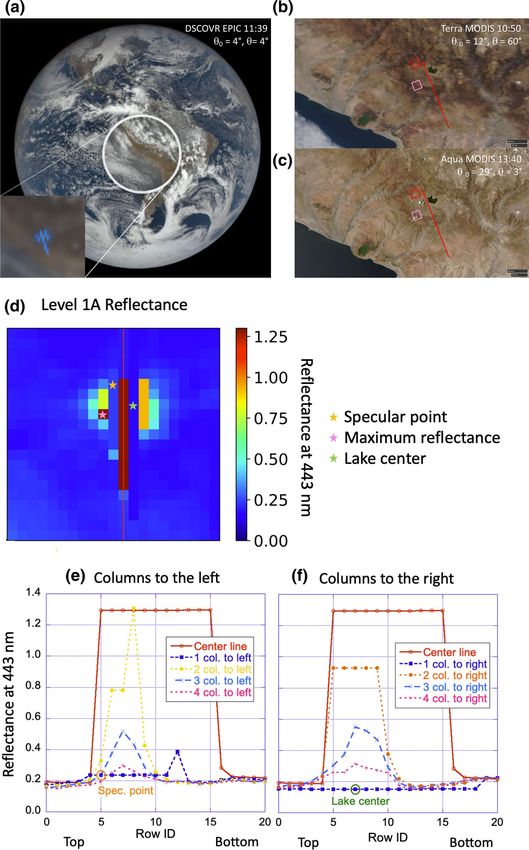
RESEARCH LETTER                            Deep Space Observations of Terrestrial Glitter
10.1029/2020EA001521
                                           Alexander Kostinski1        , Alexander Marshak2        , and Tamás Várnai2,3
Key Points:                                1
                                            Department of Physics, Michigan Technological University, Houghton, MI, USA, 2Climate and Radiation Laboratory,
• W hile most glints observed by
                                           NASA Goddard Space Flight Center, Greenbelt, MD, USA, 3Joint Center for Earth Systems Technology, University of
   EPIC come from ocean surfaces or
   ice clouds, some are found here to      Maryland Baltimore County, Baltimore, MD, USA
   originate from small lakes, high in
   the Andes
• Monitoring of global specular spots
   (terrestrial glitter) shows higher      Abstract Deep space climate observatory (DSCOVR) spacecraft drifts about the Lagrangian point
   time-averaged reflectance at specular   ≈1.4–1.6 × 10⁶ km from Earth, where its Earth polychromatic imaging camera (EPIC) observes the sun-lit
   spots than elsewhere
                                           face of the Earth every 1 to 2 hours. At any instance, there is a preferred (specular) spot on the globe,
• This specular excess reflectance
   becomes more pronounced as              where a glint may be observed by EPIC. While monitoring reflectance at these spots (terrestrial glitter),
   geolocation improves. Conversely,       we observe occasional intense glints originating from neither ocean surface nor cloud ice and we argue
   specular excess can be used to
                                           that mountain lakes high in the Andes are among the causes. We also examine time-averaged reflectance
   monitor geolocation
                                           at the spots and find it exceeding that of neighbors, with the excess monotonically increasing with
                                           separation distance. This specular excess is found in all channels and is more pronounced in the latest
Correspondence to:
                                           and best-calibrated version of EPIC data, thus opening the possibility of testing geometric calibration by
A. Kostinski,
kostinsk@mtu.edu                           monitoring distant glitter.

                                           Plain Language Summary                    We find that bright reflections of sunlight (glints) observed by a
Citation:
                                           satellite camera, a million miles away can help with accurately determining location of each image pixel.
Kostinski, A., Marshak, A., & Várnai,
T. (2021). Deep space observations         In addition to previously observed glints from the ocean surface and clouds, we detect overwhelmingly
of terrestrial glitter. Earth and Space    bright glints off high mountains in the Andes, likely caused by calm small lakes.
Science, 8, e2020EA001521. https://doi.
org/10.1029/2020EA001521

                                           1. Introduction
Received 14 SEP 2020
Accepted 25 NOV 2020                       Pixels associated with specular reflections of light (henceforth, glints) are typically the brightest in photo-
                                           graphs or satellite images. Although they occasionally serve as calibration targets in remote sensing, glint-
                                           ing pixels are frequently flagged or discarded as glints interfere with various retrievals. Yet, often the bright-
                                           est incoherent sources around, these glints contain much interesting physics and have even been suggested
                                           as beacons of exosolar planets (Robinson et al., 2010; Williams & Gaidos, 2008). To that end, this work is
                                           devoted to the study of deep space climate observatory/earth polychromatic imaging camera (DSCOVR/
                                           EPIC) glint observations of Earth, the most distant methodical observations of glints available to date.

                                           The EPIC camera onboard DSCOVR is a 10-channel spectroradiometer (317–780 nm), taking images of the
                                           entire sunlit face of Earth every one to two hours. The detector is a 2,048 × 2,048 pixel charge coupled device

                                           center is ∼10 km by 10 km and the angular spread ≈(3 × 10⁻⁴)°. Because of a rotating wheel of color filters
                                           (CCD) and images are obtained by 10 narrow band spectral channels. The typical pixel size D near the image

                                           inside the EPIC telescope, there is a time lag between the images at different wavelengths: 3 min difference
                                           between blue (443 nm) and green (551 nm), 4 min between blue and red (680 nm) and 54 s between green
                                           and red. The red green blue (RGB) images are generated daily and are available to the general public at
                                           http://epic.gsfc.nasa.gov.

                                           2. Glint Analysis
© 2021. The Authors. Earth and
Space Science published by Wiley           Many images contain variously colored bright spots as in Figure 1, caused by glints as was shown in prior
Periodicals LLC on behalf of American      work (Li et al., 2019; Marshak et al., 2017; Várnai et al., 2019). In particular, only glints over oceans were
Geophysical Union.
This is an open access article under       observed by Sagan et al. (1993) but not exclusively so in Marshak et al. (2017), where ice crystals in clouds
the terms of the Creative Commons          over land were documented as the origin of the glints. For this work, we have examined multiyear time
Attribution License, which permits use,    series of glints (terrestrial glitter), emphasizing the brightest ones, with a threshold reflectance, ρ ≥ 1.3,
distribution and reproduction in any
medium, provided the original work is      beyond which detector saturation occurred. The ρ values used here are based on the engineering units of
properly cited.                            counts per second, weighted by calibration factors for each wavelength. The calibration factors were ob-

KOSTINSKI ET AL.                                                                                                                                       1 of 8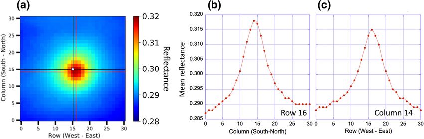
Earth and Space Science   10.1029/2020EA001521

KOSTINSKI ET AL.                                               2 of 8
Earth and Space Science 10.1029/2020EA001521
tained by comparing EPIC observations with measurements taken by low Earth orbit satellite instruments
such as moderate resolution imaging spectroradiometer (MODIS) and (OMI) ozone monitoring instrument
(Geogdzhayev & Marshak, 2018; Herman et al., 2018). Several “superglints”, with ρ ≥ 1.3, occurred over land
in Peru and Bolivia, high in the Andes (the only high mountains in tropics, where EPIC viewing geometry
permits glints) and caught our attention.
As a case study, consider a single color (blue) example of an intense detector-saturating glint (superglint) over
cloud-free land shown in Figure 1. We chose blue glint because of the highest spatial resolution, ≈8 km (Mar-
shak et al., 2018). To demonstrate cloud-free conditions, in Figure 1 we present “before” and “after” images of
the region by Terra (10:50 a.m.) and Aqua (1:40 p.m.) MODIS for the same day. These natural color composite
RGB images (MODIS bands one (red, 0.65 μm); four (green, 0.55 μm), and three (blue, 0.47 μm) show nearly
cloud-free conditions over the Andes, except for marine stratocumuli observed by Terra (see panel 1b), far
away from the specular spot (red pixel in Figure 1) and a few low-level liquid water small cumulus clouds,
observed by Aqua (see panel 1c). It is quite unlikely that ice clouds were absent at 10:50 a.m., appeared at
noon and disappeared at 1:40 p.m. See additional evidence in panels (d) and (e) of Figure 2, ruling out Cirrus.
If neither cloud ice particles nor ocean surface, what is the origin of the superglint? This raises the general
question: in the absence of clouds and ocean, what features in the mountains might produce the detector-sat-
urating superglint? Could it possibly be the small lake, visible in Google Earth approximately 40 km south-east
of the specular spot, Figures 1 and 2? Small lakes have been implicated in this context before (F.-M. Bréon &
Dubrulle, 2004; F. Bréon, 1993; F. Bréon & Deschamps, 1993) but no data of sufficient quality was obtained
to document it (Bréon, private communication.) In contrast, large lakes such as Titicaca in Peru have been
used as calibration targets by the Hyperangular Rainbow Polarimeter cubesat (Vanderlei Martins, private
communication) and airborne observations of lake glints have been well documented (Gatebe & King, 2016).
To examine the physics of the superglint more closely, we recall that multicolor glint-causing conditions
erable spatial extent as the Earth spins ∼100 km during such time. Conversely, single color glints such as
(composite image) must persist for at least 4 min (the lag between blue and red channels), implying consid-
the one in Figure 1 had been caused by briefer and more fleeting conditions. We therefore draw the reader's
attention to the snapshot, panel (d) of Figure 1, depicting the raw, Level 1A, 443 nm data alone. Locations of
particular interest are: the specular position (marked by yellow star), a stand-alone pixel of maximal reflec-
tance, marked by the pink star, (ρ ≈1.31), and another superglint where saturation appears to have occurred
as indicated by the thick straight red line, due presumably to the CCD spillage along the detector columns,
for example, (Gorkavyi et al., 2020).
Let us examine the physics of specular (singly scattered) reflection in the context of panel (d) of Figure 1.
For a single color image, most of the pixel-to-pixel reflectance (ρ) variation can be attributed to: (i) illumina-
tion conditions; (ii) differences in the effective index of refraction; and (iii) angular concentration of reflect-
ed radiation. While the first two vary by an order of magnitude or so (Rees, 2013), the last can vary by three
orders of magnitude (hence, frequent saturation from glints). Indeed, Lambertian surface scatters perfectly
facet can concentrate that singly scattered radiation into a solid angle dΩ ≈1 × 1° or ∼10−4 fraction of 2π.
diffuse radiation into an entire hemisphere, i.e., a solid angle of dΩ = 2π, whereas a smooth glint-producing
We use the 1° estimate because the angular size of the sun is ≈0.5° and so is the spread of incident sunlight.
In addition, the surface normal change across a single pixel is ≈0.1°, affecting both incidence and reflection
angles (pixel extent of ≈(3 × 10⁻⁴)° is negligible).
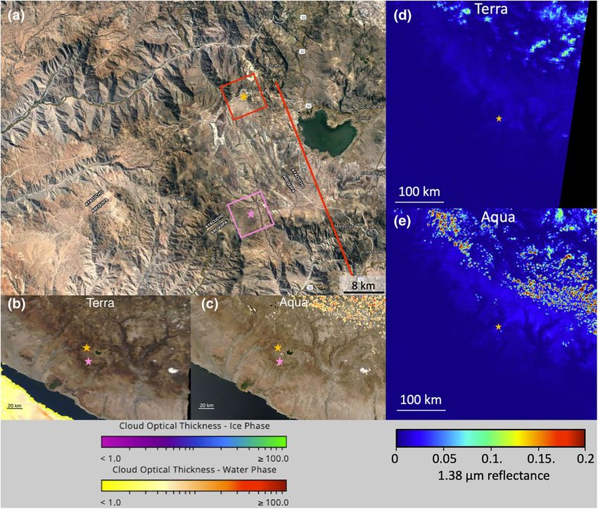
Figure 1. Superglint cause? Panel (a): Superglint from November 17, 2015, 16:39 UTC, (inset: glint is apparent in
EPIC blue channel, λ = 443 nm) with SZA = 4.04° (θ0 in legend) and VZA = 3.99° (θ) adding up to ≈8.03° versus the
SEV angle of 7.95°, implying glint-generating tilts of 0.08°. Specular spot: Latitude: 15.23°S, Longitude: 73.87°W; Panels
(b) and (c): cloud-free MODIS images of glint scene taken about an hour before and after the EPIC image, (at 15:50
UTC by Terra and at 18:40 UTC by Aqua), ruling out cloud origin of the superglint. The panel (a) image is composite
color, spanning 4 min, but panel (d) level 1A image had an exposure time of 46 msec (Herman et al., 2018), during
which the Earth spun ≈13 m. Pink square marks second reflectance (ρ) peak, likely not caused by CCD saturation
spillover. The red squares in panels (b) and (c) center on the specular spot (ρ = 1.29), demarcating EPIC pixels of ≈8 km
size that day. The extended glint is, likely, due to the mountain lake, but the other glint, pink star in panel (d), with the
maximum reflectance ρmax = 1.31, is perplexing. (See also Figure 2). Panels (e) and (f) detail the intensity distribution.
EPIC, earth polychromatic imaging camera; MODIS, moderate resolution imaging spectroradiometer; SEV, Space
Exploration Vehicle; SZA, solar zenith angle; UTC, Coordinated Universal Time; VZA, view zenith angle.
KOSTINSKI ET AL. 3 of 8Earth and Space Science 10.1029/2020EA001521
Figure 2. Absence of ice clouds at superglint locations. Panel (a): close-up Google Earth image of the high EPIC reflectance region, altitude ≈3.4 km.
Pixels are geographically positioned, with their areas demarcated by the colored squares, (7.45 km on a side, the EPIC resolution for the day of observation).
The red pixel covers the specular spot and is centered at the yellow star, whereas the pink star flags the puzzling spot of maximal reflectance where a rocky river
bed appears, possibly with streams at the time of EPIC image. The areal extent of the mountain lake is comparable to the pixel area (scale bar in the lower right
corner). Note more than a pixel separation between the red line (aligned with CCD columns) and the second superglint, suggesting that perhaps the pink star
reflectance is not merely an artifact of CCD spillage. Panels (b) and (c): Aqua and Terra MODIS cloud optical thickness (τ) maps of the scene, superimposed
on the natural color panels 1b and 1c. Infrared and visible channels contribute to τ-maps and show small subpixel clouds (yellow and red) detected there by
Aqua 1:40 p.m. local time but absent at 10:50 a.m. local time in Terra images. These clouds were classified as liquid phase by Aqua despite the relatively high
altitude. No ice clouds are found (no purple, blue, or green). Panels (d) and (e): MODIS Terra and Aqua infrared observations at 1.38 μm, particularly sensitive
to scattering by high cirrus clouds. Pink stars omitted for transparency. Because of uniformly low reflectance values (blue), neither image (before or after EPIC)
indicates presence of even a thin cirrus anywhere near the second superglint (pink star) location. CCD, charge coupled device; EPIC, earth polychromatic
imaging camera; MODIS, moderate resolution imaging spectroradiometer.
max
The image contrast min observed for the entire image of panel (d) is 1.314/0.018 = 73, but other level 1A
images occasionally attain dynamic range values of ∼103, the upper bound being set by the 12 bit (=2048)
detection system. It is the minimal ρ that varies most from image to image and in the raw (level 1A) im-
ages of the blue channel it is set by the atmospheric Rayleigh scattering (optical depth of 0.24 at 443 nm)
for pixels near the image edge, by the dark side of the Earth. In contrast, the upper bound on ρ is set by
detector saturation, the latter depending on the exposure time. The exposure time is set so that bright cloud
pixels (ρ ≈0.9) fill the potential well of the EPIC CCD detector to about 80% of its 95,000 electrons satura-
tion limit (Jay Hermann, private communication). The EPIC maximal signal-to-noise ratio (SNR) = (0.8
∼102 for a ballpark estimate, one then expects (conservatively) the glints to saturate the detector at ∼102 of
× 95,000)1/2 = 275 (at near saturated pixels), with the exposure time adjusted accordingly. Using this SNR
KOSTINSKI ET AL. 4 of 8Earth and Space Science 10.1029/2020EA001521
Figure 3. Time-averaged reflectance peak falls within one pixel of the geometric center. All three panels based on version 3, full-year 2017 data. Land
and ocean surface glints are included with all cloud glints as well and data from all 10 EPIC bands are combined here. 3,468 EPIC images were used to create
these plots. Panel (a): color-coded image of time-averaged reflectance versus the image position. Black cross-hairs meet at the specular point while red ones at
the maximum reflectance value. Reflectance values ≈0.3 in rough agreement with the Earth albedo for SW broadband; panel (b) time-averaged reflectance slice
of row 16 versus column position; panel (c) time-averaged reflectance slice of column 14 versus row position. EPIC, earth polychromatic imaging camera; SW,
Shortwave.
the perfectly diffuse Lambertian pixel value near the image edge. Therefore, an important conclusion in the
reflector with the right geometry, saturates the detector. Thus even a small calm mountain lake of ∼1 km2
present context is that a mere one percent fraction of the 100 km2 pixel area, occupied by a perfect specular
area can cause a superglint. Figures 1 and 2 confirm that we can add small lakes to cloud ice and ocean
surface as potential causes of EPIC superglints.
Discovering that small lakes can beam focused light all the way into deep space is rendered plausible by
the above back-of-the-envelope estimate. However, the second peak, flagged by the pink square in panels
1b-d and 2a-c, (ρ = 1.31) is perplexing. Could it possibly be the tiny subpixel warm cloud in the Aqua im-
ages of panels 1c and 2c? Liquid water drops, although conceivably retro-reflectors, have never been im-
plicated in specular reflections to space, to the best of our knowledge. Nor is it likely that the tiny cloud,
if misclassified by Aqua and mixed phase in reality, would have contained enough ice crystals to yield a
superglint. Indeed, it is tempting to dismiss this superglint as an instrumental artifact such as a spillage
of the incoming radiance along the columns of the CCD detector, for example, (Gorkavyi et al., 2020).
Closer inspection of panels 1 e, f reveals unrealistically steady ρ values in columns on either side of the
column, containing the main glint, with low values of ρ in the next-neighbor columns and slightly higher
but still unsaturated ρ in the second column on either side. However, panel 1 e also shows that the CCD
spillage in the second column to the left caused two neighboring pixels to have identical mid-range ρ
values whereas the second peak pixel has a much higher, saturated ρ. This permits the scenario that some
neither lake nor ice cloud feature in the area of the second peak pixel increased ρ well over the value
implied by the CCD spillage.
Therefore, we raise the admittedly far-fetched possibility that superglints could also be caused by small
features, capable of constructive interference. For example, salty deposits in Bolivia and snowy mountains
in Ecuador are within the DSCOVR observational band of latitudes. Could a superglint be a reflection from
stationary elements such as snow or salt deposits or even fleeting ones such as facets of capillary waves on
ponds (Lynch et al., 2011)? In contrast to incoherent glints, caused by angular concentration of scattered
radiation, the coherent ones would depend greatly on the exposure time, i.e., constructive interference relies
on maintaining zero relative phase between pairs of scattering elements (e.g., facets of the lake surface, or
ice crystals in clouds), throughout the time of observation.
Our argument involves both spatial and temporal coherence of scattered light (Ishimaru, 1978; Wolf, 2007).
To that end, we ask: how far should the detector be from the terrestrial image pixel, for the latter to be
considered a point source? This spatial coherence (all parts radiating in phase) condition is given by, for
example, (Crawford, 1968) [Equation 38]
KOSTINSKI ET AL. 5 of 8Earth and Space Science 10.1029/2020EA001521
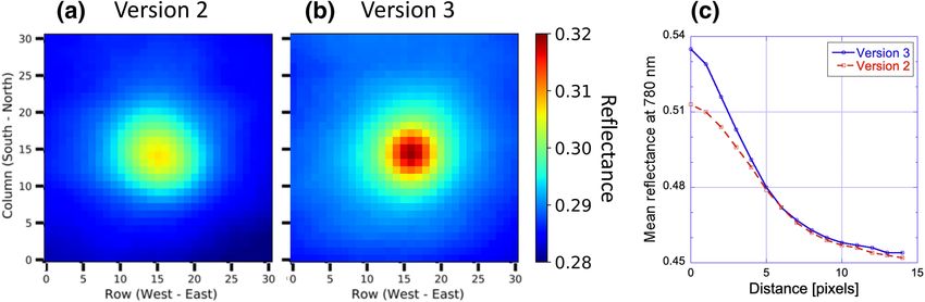
Figure 4. Reflectance excess, δρ, at the specular spot is less pronounced in version 2 (panel a) than in version 3 (panel b). δρ profile is narrower as
the variance decreases from second to third version. The positioning of the peak improved and became nearly coincident with the specular spot from first (not
shown) to second version. Hence, improved geo-location is confirmed by the diminishing random and deterministic errors. Thus glint-caused specular excess
supplies a beacon to monitor geolocation on Earth and other planets. All three panels are based on full 2017 data. Land, ocean surface and cloud glints are all
included. Data from all 10 EPIC bands are combined here for panels (a) and (b) while panel (c) curves are for 780 nm channel over land (surface and cloud).
EPIC, earth polychromatic imaging camera.
(1)
dD L
where the two transverse lengths d and D are the detector and source (pixel) sizes, respectively and the two
longitudinal length, λ and L are wavelength and Earth-satellite distance, respectively. From this perspective,
observation distance. Inserting numbers in meters gives 3 × 10−1 × 104 ∼ 0.5 × 10−6 × 1.5 × 109, yielding
EPIC/DSCOVR deep space observations are particularly interesting because of the sheer magnitude of the
∼103 for both sides. Thus, partial coherence can occur and specular areas must be smaller than the moun-
tain lake to satisfy (1), e.g., 1% of the pixel area. Next, we examine the temporal coherence of scattered
∼10 ms. These can be readily satisfied by stationary elements on the ground but not necessarily by moving
light. One condition is the constancy of relative positions of scattering facets during the exposure time of
ice crystals in clouds or capillary waves on the lake surface. The hallmark of coherence is that the scattering
intensity is quadratic rather than linear in the number of scatterers n, e.g., number of cloud ice crystals. In-
deed, the total intensity I, averaged over the exposure time (averaging over the observation time is denoted
by angular brackets) is given by
2
I [a1 t (a2 t an
(2) t ]2 a1 (t ) 2 a1 t a2 t an t
where ai are the scattering amplitudes of n elements such as facets of a capillary wave. These amplitudes
may be considered comparable for the purpose of this argument. In the incoherent case (e.g., radiative
transfer), n2 − n off-diagonal element time-averages vanish and only n diagonal terms remain so that < I >
relative cross-term magnitude ϵ is relatively small, ϵ × n2 ∼ n may still result. Although the natural coher-
is indeed additive. Not so when the exposure time is comparable to the coherence time T. Even if a typical
ence time of the filtered (width: 10 nm) incident blue light is on the order of microseconds, this discussion
pertains to the coherence acquired via scattering.
ice cloud) × 1 km × 1 km ∼108 cubic meters, with number density of 103 per cubic meter, yields n ∼1011
For instance, the number of ice crystals in a cloud volume of 100 m (one mean free path of a tenuous
δu ∼1 mm/sec and the sought coherence time T, yields T ∼10−3sec. This msec is still short compared
while the decorrelation time, estimated by setting the wavelength λ to the product of relative speed
this case, considering huge n2, partial coherence effects may be discernible if ϵn ∼1. The case is much
with the 46 msec exposure time (Geogdzhayev & Marshak, 2018) for the EPIC blue channel but even in
stronger for stationary elements such as salt grains on the ground. EPIC/DSCOVR exposure time can
vary via the adjustable slit widths and spinning rates. This allows for testing the coherent glint conjec-
ture, should opportunity arise, because, in contrast to incoherent glints, even relative coherent glint
KOSTINSKI ET AL. 6 of 8Earth and Space Science 10.1029/2020EA001521
intensity within the scene depends nonlinearly on the exposure time so
that changes in the saturation statistics would be a revealing symptom.
Such coherence-induced many-fold increase in glint intensity could
lead to detection of exosolar glitter.
We now return to the time series of glints (terrestrial glitter) but, in
contrast to earlier work (Marshak et al., 2017), here we use neither
detection algorithms nor any subjective criteria. Instead, relying on
the fundamental physics that glints can occur only where an observa-
tion of specular reflection off properly oriented facets is possible, we
monitor the reflectance versus time at these specular spots (one per
each image). Specular reflector at a given instant of observation may
be absent (e.g., the specular pixel is covered by forested land with no
lakes nor cloud cover) and then the usual diffuse component is respon-
sible for the observed pixel brightness. However, insofar as specular
reflections (glints) are always brighter than the diffuse ones, one ex-
pects time-averaged brightness at these specular spots to exceed the
Figure 5. Specular Excess is spectrally robust δρ > 0 is observed in the rest of the pixels. The key ingredients here are statistics and geometry
vicinity (14 pixels) of the specular spot for all 10 EPIC channels. Hence,
and we propose the notion of specular excess, denoted δρ as the quan-
specular excess is a statistically robust finding. Data for the entire 2017:
land surface and cloud glints. Rayleigh scattering above clouds reduces tity of interest: one expects δρ maximum at the specular position and
the excess more at the shorter wavelengths, and so does absorption by decrease toward the typical diffuse reflectance as the distance from the
oxygen (at 688 nm and 764 nm in particular) and by ozone (at 317 nm and specular spot increases. Hence, all pixels located, say, five pixels away
325 nm). EPIC, earth polychromatic imaging camera. from the global specular spot are averaged over with the associated < ρ
> below the peak value. This specular excess hypothesis is confirmed
by Figure 3, panel (a) where the red and black cross-hairs are nearly
coincident. Panels (b) and (c) of Figure 3 further show that the positioning of the maximum is within a
fraction of one pixel from the specular position.
The argument for geo-calibration by specular reflection excess statistics is further buttressed by the com-
parison of EPIC data versions. For the latest (third) version, coastlines were cross-checked with MODIS and
GOES-17 to produce superior geolocation (Karin Blank, personal communication) as illustrated in Figure 4.
Again, both images are centered to within a pixel of the reflectance maximum. Note that while the mean
location of the intensity peak does not change much from second to third version, the variance about the
mean location decreases substantially in the third version. This is a welcome finding as the smaller variance
implies that it is now less likely for random uncertainties in geolocation to cause discrepancies with the
geometric localization of specular points.
Lastly, Figure 5 demonstrates that the notion of specular excess holds for all 10 of the EPIC channels, ren-
dering the finding statistically robust. What determines the order of glint specular excess curves? Presum-
ably, the primary cause of the (land) excess is the reflection by ice clouds. Rayleigh scattering above clouds
as well as absorption by oxygen and ozone diminish δρ as the increased absorption weakens the contrast. In
other words, δρ caused by the glint contribution is least obscured by the weakest atmospheric absorption or
scattering above the glint. For example, B-band oxygen absorption (688 nm) is much weaker than A-band
absorption (764 nm) and indeed, the 688 nm curve is above the 764 nm one. Interestingly, the 688 nm curve
is also close to 443 nm curve: one due to Rayleigh scattering (443 nm) and one due to oxygen absorption
(688 nm). Aside from oxygen absorption, the rest of the curves are ordered nearly by the wavelength, in
agreement with the Rayleigh background interpretation. Our most recent findings on seasonal and spectral
aspects of glints can be found in (Várnai et al., 2020).
3. Summary
In summary, we found that even small lakes can project superglints into deep space and that such features,
in addition to being calibration targets, cause statistically steady terrestrial glitter enhancement δρ and,
thereby, can serve as beacons for monitoring geo-location. Should the coherent glint mechanism prove
viable, it has the potential for exosolar glitter, linking geoscience with astronomy.
KOSTINSKI ET AL. 7 of 8Earth and Space Science 10.1029/2020EA001521
Data Availability Statement
All DSCOVR EPIC data products are archived and publicly distributed through the NASA Langley At-
mospheric Science Data Center (ASDC). Access to any NASA Earth-viewing satellite datasets (e.g., EPIC
data) requires a NASA Earthdata account, which can be obtained by registering at https://urs.earthda-
ta.nasa.gov/. Once logged in at the URL above, the data file used for the individual case study present-
ed in this paper can be downloaded at https://asdc.larc.nasa.gov/data/DSCOVR/EPIC/L1A/2015/11/
epic_1a_20151117163941_03.h5.
The yearlong dataset used for the presented statistical analysis can be downloaded from https://asdc.
larc.nasa.gov/data/DSCOVR/EPIC/L1B/2017/.
The subdirectories at this URL are labeled 01 to 12 and contain all EPIC Level 1B data from each of
the 12 months (and contain no other files). The natural color EPIC image used for illustrating the indi-
vidual case study can be downloaded at https://epic.gsfc.nasa.gov/archive/natural/2015/11/17/png/
epic_1b_20151117163941.png
The MODIS natural color images and cloud optical thickness images used in this case study can be
viewed at https://worldview.earthdata.nasa.gov, by selecting at the bottom the date (November 17, 2015)
and then toggling at the left side the switch between MODIS images taken from the Terra and Aqua satellites.
The MODIS infrared images were extracted from the operational MODIS Level 1B radiance product
available at https://ladsweb.modaps.eosdis.nasa.gov/archive/allData/61/MOD021KM/2015/321/MOD-
021KM.A2015321.1550.061.2017321165225.hdf and at https://ladsweb.modaps.eosdis.nasa.gov/archive/
allData/61/MYD021KM/2015/321/MYD021KM.A2015321.1840.061.2018054020625.hdf
Acknowledgments References
This research was supported by the
Bréon, F. (1993). An analytical model for the cloud-free atmosphere/ocean system reflectance. Remote Sensing of Environment, 43(2),
NASA DSCOVR project and by NSF
179–192. https://doi.org/10.1016/0034-4257(93)90007-K
AGS-1639868. The authors thank W.
Bréon, F., & Deschamps, P.-Y. (1993). Optical and physical parameter retrieval from polder measurements over the ocean using an analyt-
Wiscombe for insightful comments,
ical model. Remote Sensing of Environment, 43(2), 193–207. https://doi.org/10.1016/0034-4257(93)90008-L
K. Blank for explaining geolocation of
Bréon, F.-M., & Dubrulle, B. (2004). Horizontally oriented plates in clouds. Journal of the Atmospheric Sciences, 61(23), 2888–2898. https://
version 3, and J. Herman and R. Levy
doi.org/10.1175/JAS-3309.1
for helpful discussions.
Crawford, F. S. (1968). Waves, Berkeley physics course (Vol. 3, pp. 1–600). McGraw-Hill.
Gatebe, C. K., & King, M. D. (2016). Airborne spectral BRDF of various surface types (ocean, vegetation, snow, desert, wetlands, cloud decks,
smoke layers) for remote sensing applications. Remote Sensing of Environment, 179, 131–148. https://doi.org/10.1016/j.rse.2016.03.029
Geogdzhayev, I. V., & Marshak, A. (2018). Calibration of the DSCOVR epic visible and NIR channels using MODIS terra and aqua data and
epic lunar observations. Atmospheric Measurement Techniques, 11(1), 359–368. https://doi.org/10.5194/amt-11-359-2018
Gorkavyi, N., Fasnacht, Z., Haffner, D., Marchenko, S., Joiner, J., & Vasilkov, A. (2020). Detection of non-linear effects in satellite UV/vis
reflectance spectra: Application to the ozone monitoring instrument. Atmospheric Measurement Techniques Discussions, 1–24. https://
doi.org/10.5194/amt-2020-327
Herman, J., Huang, L., McPeters, R., Ziemke, J., Cede, A., & Blank, K. (2018). Synoptic ozone, cloud reflectivity, and erythemal irradiance
from sunrise to sunset for the whole earth as viewed by the DSCOVR spacecraft from the earth; Sun Lagrange 1 orbit. Atmospheric
Measurement Techniques, 11(1), 177–194. https://doi.org/10.5194/amt-2017-155
Ishimaru, A. (1978). In Wave propagation and scattering in random media, (1–600). New York. Academic Press, 2. https://doi.org/10.1016/
B978-0-12-374701-3.X5001-7
Li, J.-Z., Fan, S., Kopparla, P., Liu, C., Jiang, J. H., Natraj, V., & Yung, Y. L. (2019). Study of terrestrial glints based on DSCOVR observations.
Earth and Space Science, 6(1), 166–173. https://doi.org/10.1029/2018EA000509
Lynch, D. K., Dearborn, D. S., & Lock, J. A. (2011). Glitter and glints on water. Applied Optics, 50(28), F39–F49. https://doi.org/10.1364/
AO.50.000F39
Marshak, A., Herman, J., Adam, S., Karin, B., Carn, S., Cede, A., et al. (2018). Earth observations from DSCOVR epic instrument. Bulletin
of the American Meteorological Society, 99(9), 1829–1850. https://doi.org/10.1175/BAMS-D-17-0223.1
Marshak, A., Várnai, T., & Kostinski, A. (2017). Terrestrial glint seen from deep space: Oriented ice crystals detected from the Lagrangian
point. Geophysical Research Letters, 44(10), 5197–5202. https://doi.org/10.1002/2017GL073248
Rees, W. G. (2013). Physical principles of remote sensing. Cambridge University Press. Retrieved from: https://waterhouse.ir/sites/default/
files/Physical%20Principles%20of%20Remote%20Sensing%20-%20Third%20Edition_0.pdf
Robinson, T. D., Meadows, V. S., & Crisp, D. (2010). Detecting oceans on extrasolar planets using the glint effect. The Astrophysical Journal
Letters, 721(1). L67–L71, https://doi.org/10.1088/2041-8205/721/1/L67
Sagan, C., Thompson, W. R., Carlson, R., Gurnett, D., & Hord, C. (1993). A search for life on earth from the galileo spacecraft. Nature,
365(6448), 715–721. https://doi.org/10.1038/365715A0
Várnai, T., Kostinski, A. B., & Marshak, A. (2019). Deep space observations of sun glints from marine ice clouds. IEEE Geoscience and
Remote Sensing Letters, 17(5), 735–739, https://doi.org/10.1109/LGRS.2019.2930866
Várnai, T., Marshak, A., & Kostinski, A. (2020). Deep space observations of sun glints: Spectral and seasonal dependence. IEEE Geoscience
and Remote Sensing Letters, 1–5. https://digitalcommons.mtu.edu/cgi/viewcontent.cgi?article=1190&context=physics-fp
Williams, D. M., & Gaidos, E. (2008). Detecting the glint of starlight on the oceans of distant planets. Icarus, 195(2), 927–937. https://doi.
org/10.1016/J.ICARUS.2008.01.002
Wolf, E. (2007). Introduction to the theory of coherence and polarization of light. 62(12), (p. 222). Cambridge University Press. https://doi.
org/10.1063/1.3047693
KOSTINSKI ET AL. 8 of 8You can also read