LIMNOLOGY OCEANOGRAPHY: METHODS
←
→
Page content transcription
If your browser does not render page correctly, please read the page content below
LIMNOLOGY
      and
OCEANOGRAPHY: METHODS                                                                                         Limnol. Oceanogr.: Methods 10, 2012, 1070–1077
                                                                                        © 2012, by the American Society of Limnology and Oceanography, Inc.

Estimating the in situ distribution of acid volatile sulfides from
sediment profile images
Peter S. Wilson* and Kay Vopel
School of Applied Sciences, Auckland University of Technology, Auckland 1142, New Zealand

         Abstract
            Measuring the sediment content of acid volatile sulfides (AVS), an important determinant of coastal ecosys-
         tem functioning, is laborious and therefore rarely considered in routine coastal monitoring. Here, we describe
         a new approach to estimate the in situ distribution of AVS in subtidal soft sediment. Using amperometric H2S
         microelectrodes and a flatbed scanner in the laboratory, we first established a strong correlation (R2 = 0.95)
         between the AVS content (as extracted by cold 1 mol L-1 HCl) and the color intensity of sediment collected at
         12 m water depth off the eastern coast of Waiheke Island, New Zealand. We then used this correlation to esti-
         mate the distribution of AVS in the upper 20 cm of this sediment from sediment profile images. These images
         were obtained in situ with a lightweight imaging device consisting of a modified flatbed scanner housed inside
         a watertight acrylic tube (SPI-Scan™, Benthic Science). We made two types of estimates from the acquired
         images: First, we obtained a vertical AVS concentration profile by averaging the color intensities of horizontal-
         ly aligned pixels. Second, we created a two-dimensional distribution plot of AVS concentration by assigning
         individual pixel color intensities. Because our technique enables assessments of temporal and spatial variations
         in the AVS content of subtidal soft sediment, we suggest using it in routine coastal monitoring.

    Enrichment of sediment with organic matter affects                    ter may be oxidized with O2 as the electron acceptor (Canfield
coastal regions worldwide. Primary causes include eutrophi-               et al. 1993a).
cation driven by anthropogenic loading of coastal waters                     The abundance of sulfate (SO42-) in the water column dic-
with phosphorus and nitrogen (Nixon 1995; Cloern 2001;                    tates that the dominant pathway for organic matter degrada-
Rosenberg et al. 2009) and deposition of organic matter via               tion in organically enriched sediments is via sulfate reduction
terrestrial runoff (Gray et al. 2002) and aquaculture (Holmer             (Thode-Andersen and Jørgensen 1989; Bagarinao 1992), which
and Kristensen 1994). The oxidation of the sediment organic               leads to the production of H2S. The overall rate of sedimentary
matter provides energy to microorganisms aided by an oxi-                 sulfate reduction responds to the rate of organic particle dep-
dizing agent (electron acceptor), the most energetically favor-           osition, that is, the supply of sulfide to coastal sediment
able being oxygen (Jørgensen and Kasten 2006). Because of                 increases with its organic carbon supply (Oenema 1990; Corn-
transport limitations (diffusion in cohesive sediment) and                well and Sampou 1995; Brüchert 1998; Sorokin and Zakuskina
low saturation concentration of oxygen in seawater, oxygen                2012). Approximately 80% (Canfield et al. 1993b) to 90%
is typically depleted within a few millimeters from the surface           (Hansen et al. 1978; Jørgensen 1982) of the sulfide is re-oxi-
of organically enriched sediment. Below this thin oxic zone,              dized, mostly through microbial activity. The remaining sul-
anaerobic bacteria use alternative electron acceptors to                  fide reacts to form more thermodynamically stable forms such
decompose organic matter (Bagarinao 1992). In Danish                      as the minerals mackinawite (FeS), greigite (Fe3S4), and pyrite
coastal sediments, for example, less than 20% of organic mat-             (FeS2), which are responsible for the black color of coastal sed-
                                                                          iments (Berner 1964; Goldhaber and Kaplan 1980; Jørgensen
                                                                          1982). Most of these sulfides convert back to H2S when treated
*Corresponding author: E-mail: peter.wilson@aut.ac.nz
                                                                          with acid and are known as acid volatile sulfides (AVS).
Acknowledgments                                                              The AVS concept was proposed by Berner in 1964. The
   The Faculty of Health and Environmental Sciences of Auckland
                                                                          author defined AVS as the sedimentary sulfur that is extracted
University of Technology funded the research, and the Earth and
Oceanic Sciences Research Institute provided field support. We thank      by 1 mol L-1 HCl, including porewater sulfides and metastable
two anonymous reviewers for their constructive critiques and com-         iron sulfide minerals such as mackinawite and greigite (Berner
ments.                                                                    1964). A variety of methods for extracting AVS have been
   DOI 10.4319/lom.2012.10.1070                                           adapted since the inception of the AVS concept, in particular,

                                                                       1070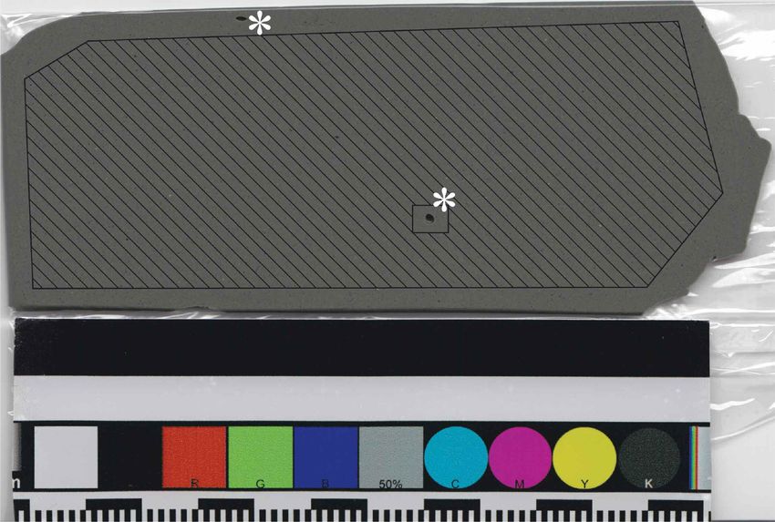
Wilson and Vopel                                                                            Estimating in situ AVS from SPI images

a range of acids, acid concentrations, and temperatures have      tubes were transported in a refrigerated box to the laboratory.
been used. Rickard and Morse (2005) raised concerns about         In the laboratory, we removed the upper lids and immersed
the uncertainty over the proportions of sulfur species            the tubes gently in a plastic container (1444 cm2 ¥ 54 cm)
extracted under these varying extraction conditions, and over     filled with 48 cm (78 L) seawater, which was aerated with a
the use of AVS as a proxy for FeS. In defense of the AVS con-     bubble stone.
cept, Meysman and Middelburg (2005) stated that despite the           Within 1 week of collection, we sectioned one sediment
simplified models, operationally defined pools like AVS and       core at a time at 5-mm intervals to a depth of 90 mm. The
organic matter have played key roles in developing our under-     upper sediment section (0–5 mm) was discarded as it was dis-
standing of sedimentary chemistry; in agreement with Luther       turbed during transport of the sediment cores. All other sedi-
III (2005), the authors concluded that the AVS concept should     ment slices were homogenized before removing 4¥ ~1 g sedi-
not be disregarded.                                               ment for AVS determination. We divided the remainder evenly
    In search of a rapid method for determining sedimentary       for the determination of sediment color intensity, water con-
AVS content, Bull and Williamson (2001) tested a new labora-      tent, organic content, and particle size distribution. We
tory approach to estimate the AVS content of estuarine sedi-      processed each slice before cutting the next, keeping the air
ment from photographs of sediment sections. They vertically       exposure of the sediment below 3 min. The effect of such
sliced sediment cores, imaged the core section with film pho-     exposure on the oxidation of AVS compounds is negligible
tography and studio lighting, and analyzed the AVS content of     (Williamson et al. 1999; van Griethuysen et al. 2002).
sediment collected from arbitrary points of the exposed sec-      AVS determination
tion. The authors extracted and quantified AVS with an acid           We added each of the four samples from a sediment slice
microdiffusion method and an ion-selective electrode              (see above) into a 40 mL glass vial filled with 30 mL HCl
(Williamson et al. 1999). These techniques revealed a weak        (1 mol L-1, ACS grade) that was deoxygenated by purging with
linear correlation (R2 = 0.67) between AVS concentration and      nitrogen for ≥ 20 min. The vial was closed with an airtight lid
sediment color intensity, but the authors believed that the       and briefly shaken. We weighed each HCl filled vial before and
actual relationship between AVS concentration and sediment        after adding sediment to determine the mass of sediment used
color intensity was stronger than their data suggested.           in the extraction. We left the vials to stand while sectioning
    One opportunity to increase the strength of the AVS con-      the remainder of the core. The sediment sampling was com-
centration–color intensity correlation lies in the choice of      pleted within 1 h.
methods used to quantify AVS and sediment color intensity.            We used an amperometric H2S microelectrode (Unisense
Here, we explore this opportunity to develop an approach for      A/S, 500-µm tip diameter, response time ~1 s) to measure the
the assessment of subtidal soft sediment. Our first goal was to   concentration of H2S in the HCl extractant. The microelec-
test if substituting laboratory film photography with digital     trode is filled with a ferricyanide solution (K3[Fe(CN)6]) that is
imaging, and modifying the analytical method for sulfide          reduced to ferrocyanide (K4[Fe(CN)6]) in the presence of H2S,
quantification, resulted in a stronger correlation between sed-   which diffuses from the surrounding HCl extractant through
iment AVS content and color intensity. Our second goal was to     the silicone membrane of the microelectrode tip (Jeroschewski
demonstrate that an automated image analyzing procedure           1996; Kühl et al. 1998). A current, linearly proportional to the
can estimate the in situ distribution of AVS from images          concentration of H2S, is produced when the reduced ferro-
obtained with a lightweight sediment profile-imaging device       cyanide is re-oxidized. The microelectrode was calibrated with
(SPI-Scan™, Benthic Science).                                     freshly prepared sulfide standards. To prepare the standards, 0,
                                                                  150, 250, and 350 µmol L-1, aliquots of a stock solution of
Materials and procedures                                          Na2S·9H2O (0.1 mol L-1) were added to 30 mL deoxygenated
    In the following, we describe a procedure that consists of    HCl (1 mol L-1). The concentration of sulfide in the stock solu-
two steps: (1) we analyzed soft subtidal sediment in the labo-    tion was measured by iodometric titration using standard
ratory to correlate sediment AVS concentration with color         iodine (0.05 mol L-1) and sodium thiosulfate (0.1 mol L-1) solu-
intensity. We refer to this step as the calibration. (2) We       tions (Vogel 1989).
applied the established AVS concentration–color intensity cor-    Color analysis
relation to sediment profile images, obtained in situ, to esti-       We scanned each homogenized sediment sample with a
mate the two-dimensional distribution of AVS.                     flatbed scanner (CanoScan LiDE 100, Canon) at a resolution of
Calibration: Correlating AVS content and color intensity          600 dpi (0.04 mm pixel-1). The flatbed scanner illuminated the
    We collected seven cores of soft subtidal sediment using      sediment with LEDs. A color calibration strip was scanned
SCUBA from an arbitrary location in Man o’War Bay, Waiheke        alongside the sediment (shown in Fig. 1). The resulting image
Island, New Zealand at a water depth of 12 m. The tubes were      was imported into the software analySIS FIVE LS Research 3.3
pushed vertically into the sediment until two-thirds were         (Olympus Soft Imaging Solutions), and color analysis was
filled with sediment and then sealed with stoppers on both        automated using a macro (details shown in Web Appendix A):
ends to minimize sediment disturbance. The sediment-filled            The intensity channel of the sediment profile image was

                                                              1071
Wilson and Vopel Estimating in situ AVS from SPI images
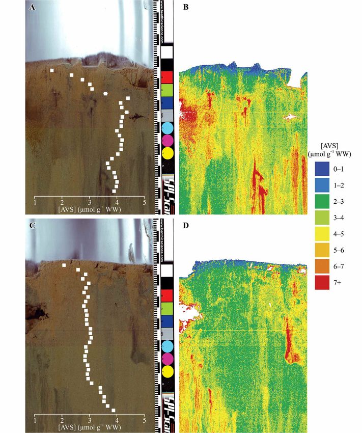
Fig. 1. An example image of a homogenized sample of soft, subtidal sediment and a color calibration strip obtained with a flatbed scanner. We used
the shaded area to measure the average sediment color intensity. The white asterisks show the locations of air bubbles that we excluded from the mea-
surement.
extracted as defined by the hue, saturation, and intensity (HSI) (Minitab Inc., v. 16.1.0). We chose to place color intensity on
color space, creating a gray-scale image. the x-axis as the error associated with this measurement will
A 4 ¥ 4 pixel averaging filter was applied to the entire image be very small; over 100,000 pixels are averaged to obtain the
to minimize the effects of noise and anomalies in the image. gray value, whereas only four measurements are averaged to
The gray-scale range of the image was adjusted linearly to obtain the AVS concentration. This configuration will produce
cover the maximum available value range, that is, the black the most representative regression using optimized least
and white calibration squares at the bottom of the image (Fig. squares.
1) were assigned values of 0 and 255, respectively. The bright- Application: In situ SPI analysis
est 2% and darkest 2% of the pixels were ignored during this We used the AVS–color intensity correlation established by
step as some images contained artifacts that were brighter or the procedure described above to estimate the in situ distribu-
darker than the calibration strip, voiding this step. tion of AVS by means of analyses of sediment profile images.
We then averaged the intensity values over the entire sam- To obtain profile images of the sediment, we deployed a sedi-
ple, approximately 50 cm2, excluding anomalies such as air ment-profile imaging device (SPI-Scan, Fig. 2) consisting of a
bubbles (see Fig. 1), to obtain an average gray value. modified consumer flatbed scanner (CanoScan LiDE 25,
Data analysis Canon; c.f. scanner used in the laboratory, CanoScan LiDE
We verified the normality of the AVS and color intensity 100), housed inside a polycarbonate cylinder (8.5 cm diame-
data individually with the Anderson–Darling test and applied ter, 28 cm length). The electrical components are contained in
a quadratic fit using color intensity on the x-axis and AVS con- a larger elliptical body (42 ¥ 30 ¥ 8 cm, hereafter, electronics
centration as the on the y-axis, with the software Minitab housing) attached to the top of the cylinder. The scanner
1072Wilson and Vopel Estimating in situ AVS from SPI images
trations into 1 µmol g-1 wet weight sediment (hereafter, µmol
g-1 WW) ranges and assigned colors from blue through to red
for low to high concentrations (Fig. 3B and D, color assign-
ment details available in Web Appendix A).
To generate a vertical AVS concentration profile (overlaid
on Fig. 3A and C), we defined a rectangular area, excluding
major anomalies such as air bubbles. The analySIS software
then calculated the average gray value for every row of pixels
within this area. Following this step, we averaged the average
gray values of 50 rows, approximately 4.2 mm, to produce one
data point. This step was used to reduce the number of data
points in the profile. Finally, we converted the average gray
values to AVS concentrations with the previously derived cor-
relation equation.
Assessment
Calibration: Correlating AVS content and color intensity
The sediment’s water content, determined by drying at
90°C for 24 h, decreased from 75% in the upper layer to 65%
at a depth of 9 cm. Its organic content, determined as weight
loss after combustion in a furnace for 6 h at 400°C, was 6.3 ±
0.9% (dry weight, mean ±SD, n = 54). Particle size (% volume)
analysis with a laser-based particle analyzer (Malvern Master-
sizer 2000) revealed that the upper 9 cm of the sediment were
comprised of 9% clay, 73% silt, and 17% sand (based on the
Wentworth scale).
The H2S microelectrode responded linearly (minimum R2 =
Fig. 2. A prototype sediment profile imaging device (SPI-Scan™, Benthic 0.991) to H2S concentration. The measurement of one extract
Science) used in this study to acquire sediment profile images. (A) Electri-
cal tether that connects the device to a 24 V power source and computer
was completed in ~10 s. The H2S concentrations in the extract
on the surface; (B) scanner electronics housing; (C) scan head; (D) frame. ranged from 4 to 350 µmol L-1, which corresponded to 0.14 to
5.01 µmol AVS g-1 WW. Statistical outliers within the four AVS
measurements per sediment slice were identified with Grubb’s
moves along the inner surface of the cylinder over a horizon- outlier test and removed.
tal distance of 120 mm to acquire a sediment image. A color The color intensity of the homogenized sediment from
calibration strip, identical to the one used in the laboratory, is each slice was derived from the average gray value of ~200,000
attached to the outside the cylinder and included in every pixels (see “Methods and procedures”). The average 95% con-
scan. The combined weight of the device and frame is ~20 kg, fidence interval of this measurement was 0.006 ± 0.001 gray
making it considerably lighter than traditionally used sedi- values (mean ±SD, n = 117).
ment imaging devices such as REMOTS, which weighs ~60 kg A quadratic function best described the relationship
(Rhoads and Cande 1971; Rhoads and Germano 1982; Rosen- between sediment AVS concentration and color intensity (R2 =
berg et al. 2001; Solan and Kennedy 2002). The depth to 0.95, Fig. 4). The average 95% individual confidence interval
which the cylinder penetrated the sediment was adjusted by was 0.531 ± 0.005 µmol AVS g-1 WW (mean ±SD, n = 117).
attaching 4 ¥ 1 kg weights to the electronics housing so that Application: In situ SPI and analysis
the sediment–water interface was approximately one-third of The established correlation between sediment AVS content
the distance from the top of the sediment profile image. An and color intensity was applied to sediment profile images
electrical tether connected the device to a 24 V power supply obtained as described above. The SPI-Scan imaged an area
and a computer on the boat. (including sediment and water column) of 117 ¥ 216 mm at a
Sediment profile images were analyzed using the same 3- resolution of 300 dpi (0.08 mm pixel-1) within 60 s.
step automated procedure used to analyze images of the sedi- The scan of the sediment profile was started immediately
ment in the laboratory (see above). An additional step was after the device was in place to exclude possible effects of the
added to the macro to produce a false-color image. The false- movement of the scan head inside the sediment on the sedi-
color image was generated by assigning the gray value of each ment profile image. Such movement could result from the
pixel to the corresponding AVS concentration with the previ- pull of the attached tether due to strong currents or boat drift.
ously derived correlation equation. We grouped AVS concen- The sediment profile images shown in Fig. 3A and C con-
1073Wilson and Vopel Estimating in situ AVS from SPI images
Fig. 3. (A and C) Two examples of sediment profile images obtained with the SPI-Scan in Sep 2010 from Man o’War Bay, Waiheke Island, New Zealand.
Small black and white bars on the scale to the right of each image are 1 mm; the larger bars are 10 mm. The images are overlaid with vertical AVS con-
centration ([AVS], µmol g-1 wet weight) profiles derived from image analysis. The error bars that are visible denote the 95% confidence interval. (B and
D) Two-dimensional AVS distribution plots derived from the images A and C, respectively.
1074Wilson and Vopel Estimating in situ AVS from SPI images
intervention, by the previously described analySIS macro
(details in Web Appendix A).
Discussion
We found a strong correlation (R2 = 0.95, see Fig. 4)
between the AVS content of soft subtidal sediment and the
sediment’s color intensity. Given the predictive power of this
correlation and the simplicity of the procedure, we believe
that estimating the distributions of AVS from sediment profile
images can become a powerful tool in the routine assessment
of subtidal organically enriched sediment, for example, sedi-
ments underneath and in the vicinity of marine farms, in
ports, or polluted estuaries. The collection of sediment cores is
only required for the initial calibration (AVS–color intensity
correlation); this makes large-scale AVS surveys possible. Fur-
thermore, our approach enables us to study how processes
such as bioturbation and particle resuspension effect the
micro-scale distribution of AVS in the upper 20 cm of sedi-
ment.
Estimating AVS from sediment profile images relies on the
assumptions that all AVS compounds are colored and that all
colored AVS compounds are quantitatively extracted. Two
Fig. 4. A scatter plot showing the relationship between the AVS con- pools do not comply with these assumptions. First, the color-
centration (µmol g-1 wet weight) and color intensity of soft, subtidal sed- less dissolved sulfide species, of which the main contributors
iment (upper 9 cm) collected from Man o’War Bay, Waiheke Island, New are H2S and HS-, are included in the acid extraction but impos-
Zealand. A color intensity of 0 is black, and that of 255 is white. The solid sible to detect using visible light. Second, some colored sulfide
line is a quadratic fit through all points ([AVS] = 0.002x2 – 0.521x + 34.3,
minerals are not extracted quantitatively, if at all. For exam-
R2 = 0.95); the 95% confidence interval is shown by the dashed lines on
either side. ple, cold 1 mol L-1 HCl does not extract pyrite, and only
extracts ~40% to 67% of greigite and 92% of mackinawite
(Rickard and Morse 2005). This nonquantitative extraction
tained an artifact caused by the instrument that can be seen may render AVS concentration estimates inaccurate if the rel-
from the top of the image down to the cyan circle. The color ative concentrations of these pools were to change either tem-
property affected by this artifact was hue, with the exception porally or spatially. The formation of pyrite in organically
of a narrow band level with the 50% gray calibration square. enriched sediments may be impeded according to Morse and
Because the majority of this artifact did not affect our AVS esti- Wang (1997). The authors reported an increased reaction rate
mates, correction of the profile images was not necessary. The between dissolved sulfide and iron (hydr)oxide (goethite), but
effect of the narrow band can be seen as an increased error of a significant decrease in the rate of pyrite formation when
the average AVS concentration derived from gray values of organic matter was present. Reduced formation of pyrite
pixels in this area. The AVS content was determined by image results in a larger proportion of sulfur species that, unlike
analysis using the previously established correlation between pyrite, are both colored and acid extractible. The possible con-
sediment AVS concentration and color intensity. tribution of colorless sulfides to AVS and incomplete extrac-
The vertical AVS concentration profile derived from the tion of some colored sulfides warrant further investigation,
sediment profile image in Fig. 3A ranged from 1.6 µmol g-1 and need to be considered before replacing time consuming
WW in the top 4 mm of sediment to 4.4 µmol g-1 WW at a AVS analysis with sediment profile image analysis. A third
depth of 30 mm. Similarly, analysis of the sediment profile issue for future consideration is the role of colored non-AVS
image in Fig. 3C resulted in a vertical AVS concentration pro- components, such as organic debris. Large components could
file ranging from 2.1 µmol g-1 WW in the top 4 mm of sedi- be excluded from the sediment image analyses and therefore
ment to 3.9 µmol g-1 WW at a depth of 140 mm. not influence the calibration procedure.
Producing an average vertical AVS concentration profile by Our data are best represented by a quadratic function (n =
analysis of a sediment profile image required ~5 min. In con- 117, R2 = 0.95). This is at variance with the linear relationship
trast, producing one average AVS profile by sectioning a sedi- (n = 40, R2 = 0.62) published by Bull and Williamson (2001).
ment core and extracting AVS with acid in the laboratory Inspection of the fit in Fig. 4 revealed an increased slope at
required ~2 h. The two-dimensional AVS distribution plots, lower color intensities, that is, the technique is less sensitive at
shown in Fig. 3B and D, were derived in ~1 s, with no user higher AVS concentrations. One possible cause for this differ-
1075Wilson and Vopel Estimating in situ AVS from SPI images
ence in sensitivity is the nonquantitative extraction of colored sediment content of dissolved colorless and non-extractable
sulfide minerals. The highest concentrations of AVS were colored minerals may not be as important as the ability to
obtained from dark-colored samples that likely contained a track temporal and spatial change in the colored AVS content.
larger proportion of the minerals mackinawite and greigite, One possible application for this technique is in the assess-
which are not quantitatively extracted. ment of the effects of aquaculture farms on benthic ecosystem
To compare our AVS concentration estimates with that in function. In this example, two factors are of interest: first,
Bull and Williamson (2001) we expressed our measured wet temporal changes in the size of the affected area of seafloor,
sediment AVS content per dry weight sediment and applied a that is, the area at which the sediment AVS content is larger
linear fit to describe the relationship between this content and than that of the background. Time-series of sediment profile
the corresponding gray values (AVS concentration = -0.323 ¥ images taken along transects that intersect the farm will reveal
color intensity + 38.8; R2 = 0.93). To do so, we assumed that such change. Second, changes over time in the intensity of the
the porewater was free of sulfides, and that the sediment water impact, that is, the maximum concentration of sedimentary
content decreased linearly from 75% wet weight in the surfi- AVS, can be revealed from the same time-series. The small size
cial layer to 65% wet weight at a depth of 9 cm. The compar- of the SPI-Scan and the rapid scanning and image analyzing
ison revealed that, for a color intensity range of 80–120, our procedure will ideally be suited to assess sediment underneath
correlation predicted AVS concentrations 2.3 µmol g-1 dry and in the vicinity of, for example, closely spaced long-lines
weight higher on average than that used by Bull and or fish cages.
Williamson (2001). Despite the differences in sediment type
(intertidal estuarine versus subtidal coastal), color determina- References
tion, and AVS quantification, these estimates are surprisingly Bagarinao, T. 1992. Sulfide as an environmental factor and
similar. This indicates that the correlation between AVS con- toxicant: Tolerance and adaptations in aquatic organisms.
tent and sediment color intensity may be valid for a variety of Aquat. Toxicol. 24:21-62 [doi:10.1016/0166-445X(92)
sediment types in the Auckland region, one prerequisite for 90015-F].
large-scale spatial surveys. Future studies may determine Berner, R. A. 1964. Distribution and diagenesis of sulfur in
whether this correlation holds for sediments outside the Auck- some sediments from the Gulf of California. Mar. Geol.
land region. 1:117-140 [doi:10.1016/0025-3227(64)90011-8].
Bull and Williamson (2001) identified precise color repro- Brüchert, V. 1998. Early diagenesis of sulfur in estuarine sedi-
duction as their primary concern. Their process of vertically ments: The role of sedimentary humic and fulvic acids.
slicing sediment cores in the laboratory, taking photographs Geochim. Cosmochim. Acta 62:1567-1586 [doi:10.1016/
under studio lighting using film photography, developing the S0016-7037(98)00089-1].
film, and digitizing the photographs introduced errors in the Bull, D. C., and R. B. Williamson. 2001. Prediction of principal
reproduction of sediment color. We minimized oxidation of metal-binding solid phases in estuarine sediments from
the sediment by horizontally slicing the sediment core so that color image analysis. Environ. Sci. Technol. 35:1658-1662
only a small portion of the sediment was exposed to air for a [doi:10.1021/es0015646].
short time (< 3 minutes). Using a flatbed scanner in the labo- Canfield, D. E., and others. 1993a. Pathways of organic carbon
ratory, we could eliminate color reproduction issues intro- oxidation in three continental margin sediments. Mar.
duced by film photography and photo digitization. The scan- Geol. 113:27-40 [doi:10.1016/0025-3227(93)90147-N].
ning hardware used in the laboratory and in situ used the ———, B. Thamdrup, and J. W. Hansen. 1993b. The anaerobic
same LEDs, creating reproducible lighting conditions; individ- degradation of organic matter in Danish coastal sediments:
ual scanning devices, however, may differ in their reproduc- Iron reduction, manganese reduction, and sulfate reduc-
tion of colors. To account for such differences, we included a tion. Geochim. Cosmochim. Acta 57:3867-3883
color calibration strip in every image so that we could adjust [doi:10.1016/0016-7037(93)90340-3].
color properties before image analysis. Cloern, J. E. 2001. Our evolving conceptual model of the
coastal eutrophication problem. Mar. Ecol. Prog. Ser.
Comments and recommendations 210:223-253 [doi:10.3354/meps210223].
The key elements of this method are the correlation of sed- Cornwell, J. C., and P. A. Sampou. 1995. Environmental con-
iment AVS content and sediment color intensity in the labo- trols on iron sulfide mineral formation in a coastal plain
ratory, and the application of this correlation to in situ sedi- estuary, p. 224-242. In M. A. Viaravamurthy and M. A. A.
ment profile images. Alternative instruments could be used to Schoonen [eds.], Geochemical transformations of sedimen-
produce similar results but it is essential that the same color tary sulfur. ACS Symposium Series. ACS Symposium, 612.
measured in situ is assigned the same color value in the labo- Goldhaber, M. B., and I. R. Kaplan. 1980. Mechanisms of sul-
ratory. Color calibration strips have been essential in this fur incorporation and isotope fractionation during early
method for color correction. diagenesis in sediments of the Gulf of California. Mar.
For the purpose of monitoring, accurately estimating the Chem. 9:95-143 [doi:10.1016/0304-4203(80)90063-8].
1076Wilson and Vopel Estimating in situ AVS from SPI images
Gray, J. S., R. S.-S. Wu, and Y. Y. Or. 2002. Effects of hypoxia ism–sediment relations using sediment profile imaging: an
and organic enrichment on the coastal marine environ- efficient method of remote ecological monitoring of the
ment. Mar. Ecol. Prog. Ser. 238:249-279 [doi:10.3354/meps seafloor (REMOTS™ system). Mar. Ecol. Prog. Ser. 8:115-128
238249]. [doi:10.3354/meps008115].
Hansen, M. H., K. Ingvorsen, and B. B. Jørgensen. 1978. Mech- Rickard, D., and J. W. Morse. 2005. Acid volatile sulfide (AVS).
anisms of hydrogen sulfide release from coastal marine sed- Mar. Chem. 97:141-197 [doi:10.1016/j.marchem.2005.08.004].
iments to the atmosphere. Limnol. Oceanogr. 23:68-76 Rosenberg, R., H. C. Nilsson, and R. J. Diaz. 2001. Response of
[doi:10.4319/lo.1978.23.1.0068]. benthic fauna and changing sediment redox profiles over a
Holmer, M., and E. Kristensen. 1994. Organic matter mineral- hypoxic gradient. Estuar. Coast. Shelf Sci. 53:343-350
ization in an organic-rich sediment: Experimental stimula- [doi:10.1006/ecss.2001.0810].
tion of sulfate reduction by fish food pellets. FEMS Micro- ———, M. Magnusson, and H. C. Nilsson. 2009. Temporal and
biol. Ecol. 14:33-44 [doi:10.1111/j.1574-6941.1994.tb00088.x]. spatial changes in marine benthic habitats in relation to
Jeroschewski, P. 1996. An amperometric microsensor for the the EU Water Framework Directive: The use of sediment
determination of H2S in aquatic environments. Anal. profile imagery. Mar. Pollut. Bull. 58:565-572 [doi:10.1016/
Chem. 68:4351-4357 [doi:10.1021/ac960091b]. j.marpolbul.2008.11.023].
Jørgensen, B. B. 1982. Mineralization of organic matter in the Solan, M., and B. Kennedy. 2002. Observation and quantifica-
sea bed—the role of sulphate reduction. Nature 296:643- tion of in situ animal-sediment relations using time-lapse
645 [doi:10.1038/296643a0]. sediment profile imagery (t-SPI). Mar. Ecol. Prog. Ser.
———, and S. Kasten. 2006. Sulfur cycling and methane oxi- 228:179-191 [doi:10.3354/meps228179].
dation, p. 271-308. In H. D. Schulz and M. Zabel [eds.], Sorokin, Y. I., and O. Y. Zakuskina. 2012. Acid-labile sulfides in
Marine geochemistry. Springer. shallow marine bottom sediments: A review of the impact
Kühl, M., C. Steuckart, G. Eickert, and P. Jeroschewski. 1998. A on ecosystems in the Azov Sea, the NE Black Sea shelf and
H2S microsensor for profiling biofilms and sediments: NW Adriatic lagoons. Estuar. Coast. Shelf Sci. 98:42-48
Application in an acidic lake sediment. Aquat. Microb. [doi:10.1016/j.ecss.2011.11.020].
Ecol. 15:201-209 [doi:10.3354/ame015201]. Thode-Andersen, S., and B. B. Jørgensen. 1989. Sulfate reduc-
Luther III, G. W. 2005. Acid volatile sulfide—A comment. Mar. tion and the formation of 35S-labeled FeS, FeS2, and S0 in
Chem. 97:198-205 [doi:10.1016/j.marchem.2005.08.001]. coastal marine sediments. Limnol. Oceanogr. 34:793-806
Meysman, F. J. R., and J. J. Middelburg. 2005. Acid-volatile sul- [doi:10.4319/lo.1989.34.5.0793].
fide (AVS)—A comment. Mar. Chem. 97:206-212 van Griethuysen, C., F. Gillissen, and A. A. Koelmans. 2002.
[doi:10.1016/j.marchem.2005.08.005]. Measuring acid volatile sulphide in floodplain lake sedi-
Morse, J. W., and Q. Wang. 1997. Pyrite formation under con- ments: Effect of reaction time, sample size and aeration.
ditions approximating those in anoxic sediments: II. Influ- Chemosphere 47:395-400 [doi:10.1016/S0045-6535(01)
ence of precursor iron minerals and organic matter. Mar. 00314-9].
Chem. 57:187-193 [doi:10.1016/S0304-4203(97)00050-9]. Vogel, A. I. 1989. Vogel’s textbook of quantitative chemical
Nixon, S. W. 1995. Coastal marine eutrophication: a defini- analysis, 5th ed. Revised by G. H. Jeffery et al. John Wiley
tion, social causes, and future concerns. Ophelia 41:199- & Sons.
219. Williamson, R. B., R. J. Wilcock, B. E. Wise, and S. E. Pickmere.
Oenema, O. 1990. Sulfate reduction in fine-grained sediments 1999. Effect of burrowing by the crab Helice crassa on chem-
in the Eastern Scheldt, southwest Netherlands. Biogeo- istry of intertidal muddy sediments. Environ. Toxicol.
chemistry 9:53-74 [doi:10.1007/BF00002717]. Chem. 18:2078-2086 [doi:10.1897/1551-5028(1999)018
Rhoads, D. C., and S. Cande. 1971. Sediment profile camera 2.3.CO;2].
for in situ study of organism–sediment relations. Limnol. Submitted 20 March 2012
Oceanogr. 16:110-114 [doi:10.4319/lo.1971.16.1.0110]. Revised 18 October 2012
———, and J. D. Germano. 1982. Characterization of organ- Accepted 18 November 2012
1077You can also read