Formal Verification of Netlog Protocols
←
→
Page content transcription
If your browser does not render page correctly, please read the page content below
Formal Verification of Netlog Protocols
                             Meixian Chen                                          Jean-François Monin
                       Dpt of Computer Science,                                   LIAMA & VERIMAG
                      Shanghai Jiao Tong University                          Université de Grenoble 1 & CNRS
                            Shanghai, China                                           Grenoble, France
                        misam.chen@sjtu.edu.cn                                 jean-francois.monin@imag.fr

   Abstract—Data centric languages, such as recursive rule based       [9], [10]. As far as we know, all these works consider systems
languages, have been proposed to program distributed appli-            modeled at a rather low level of abstraction.
cations over networks. They greatly simplify the code, while              However, a new trend on distributed programming based
still admitting efficient distributed execution, including on sensor
networks. From previous work [1], we know that they also               on data-base concepts has been proposed [11], [12], [13],
provide a promising approach to another tough issue about              [14]. In particular, Netlog [14] provides a framework which
distributed protocols: their formal verification. Indeed, we can       is both data-centric and high-level: programs are expressed by
take advantage of their data centric orientation, which allows         means of Datalog rules augmented with information on the
us to explicitly handle global structures such as the topology of      location and the transmission of facts. This greatly simplifies
the network. We illustrate here our approach on two non-trivial
protocols and discuss its Coq implementation.                          the code, while still admitting efficient distributed execution.
                                                                       From previous work [1], we know that such languages also
  Keywords-formal verification; Coq; distributed algorithms;           provide a promising approach to the verification of distributed
                                                                       protocols.
                       I. I NTRODUCTION                                   We present here the encoding in Coq of the framework
                                                                       defined in [1], and we extend it in order to take non-monotonic
   In the distributed setting, the certification of software sys-      features of Netlog into account. This includes a general library
tems turned out to be substantially more difficult than in the         formalizing a distributed computation model based on message
centralized setting. One reason is that the brute application          passing with either synchronous or asynchronous behavior, a
of the state-oriented verification technology developed for            representation of declarative rules of the Netlog language as
sequential systems to distributed systems does not naturally fit       well as their evaluation mechanism. As running examples, we
all features of the latter, making things unnecessarily complex.       consider a distributed algorithm which computes a breadth-
For instance, processes actually don’t read or write in arbitrary      first search (BFS) tree in a graph in the synchronous variant
parts of the global state. And it is certainly not accidental that     of Netlog and an optimized distributed version of Prim-
in the last two decades, much research on formal methods               Jarnìk algorithm (often referred to as Prim’s algorithm [15],
for distributed systems moved the focus from states to events.         [16]), which computes a minimum-weight spanning tree in the
Well-developed formalisms studied in this area include process         asynchronous variant of Netlog. Though these case studies are
algebra, process calculi, extended communicating automata or           simpler than GHS, they already involve subtle reasoning steps
transition systems and temporal logic. Typical issues include          and allow us to validate our framework.
stuttering, fairness, non-determinism, deadlock freedom, dis-             As for [1], our results are supported by a Coq development
tributed consensus and, more recently, mobility. Several verifi-       available in [17]. The main differences and improvements with
cation tools for event-oriented properties have been developed         relation to [1] are as follows:
and applied to different case studies, e.g., [2], [3], [4].               • We provide the intuitive ideas on the reasoning behind
   Still, many problems raised by distributed algorithms are                 the (rather dry) proof of BFS given in [1], and make it
hard to deal with in an event-oriented setting when, precisely,              more accurate using local reasoning. Let us emphasize
states play an essential role. A well-known example is the                   that the use of a proof-assistant was of much help when
distributed algorithm for computing a minimum-weight span-                   analyzing our initial proof.
ning tree due to Gallager, Humblet and Spira [5]. Rigorous                • The Coq encoding of the main definitions is presented
proofs made between 1987 and 2006 for GHS [6], [7], [8]                      here and related to the more informal style used in [1];
are all intricate and very long (100 to 170 pages). Only [7]                 additionally, we explain how Netlog rules are encoded
has been mechanically proof-checked. The point is that we                    (Section III-B).
need to reason on a global shape and, more generally, on                  • Non-monotonic features of Netlog are considered (the
data distributed on many locations. The very statement of                    deletion of facts stored on a node): the change on the
the problem already involves a global view on pieces of data                 general model is small (the definition of a local round)
located at various locations in the system. This can be seen on              but the impact on proof scripts is more important, our
previous work performed with the ACL2 proof-assistant, e.g.,                 complete development about BFS was upgraded accord-
ingly in order to update the methodology. Section IV. Aggregation functions, such as min in the next
• A non-trivial distributed version of Prim’s algorithm is example, can also be used in the head of rules to aggregate
provided, as well as a manual correctness proof. The over all values satisfying the body of the rule.
reasoning is much more involved than for BFS; its for- Let us consider next, the construction of a BFS tree for
malization in Coq using the techniques described earlier synchronous systems. The following program relies on three
is started. relation symbols: E, onST , and ST ; E represents the edge
The rest of this paper is organized as follows. Section relation; and at any stage of the computation, onST (α)
II recalls the Netlog language, illustrates it with BFS and (respectively ST (α, β)) holds iff the node α (respectively the
discusses the proof of the correctness of BFS. Section III edge (α, β)) is already on the intended tree.
presents our Coq formalization of Netlog. Section IV is Synchronous Rooted BFS Tree
dedicated to Prim’s algorithm and its correctness proof. We
l onST (x) ← @x = 0. (1)
conclude in Section V.
l onST (y)
← E(x, @y); onST (x); ¬onST (y). (2)
II. P ROVING A D ISTRIBUTED A LGORITHM IN N ETLOG ↓ ST (min(x), y)
A. The Netlog Language
Rule (1) is enabled on the unique node, say ρ, which satisfies
Only the main constructs of Netlog are presented. A more the relation ρ = 0. It derives a fact OnST (ρ), which is stored
thorough presentation of the language can be found in [14]. on ρ and sent to its neighbors. Rule (2) runs on the nodes
Netlog relies on datalog-like recursive rules, of the form (@y) at the border of the already computed tree. It chooses
head ← body, which allow to derive the fact “head” whenever one parent (the one with minimal Id) to join the tree. Two facts
the“body” is satisfied. In contrast with other approaches to are derived, which are both locally stored. The fact onST (y)
concurrency, the focus is not, primarily, on observing some is pushed to all neighbors. Each fact E(x, y) is assumed to
output, but on the high-level data (i.e. datalog facts) contained be initially stored on node y. As no new fact E(x, y) can be
in nodes. Imagine, for example, a program for constructing derived from rules (1) and (2), the consistency of E with the
routing tables. Such tables are intended to be used by other physical edge relation holds forever.
protocols and reasoning on their contents is more direct than This algorithm aims at constructing a suitable distributed
considering events. relation ST . More precisely, we prove below that the relation
The Netlog programs are installed on each node, where they ST actually defines a BFS tree.
run concurrently. Deduced facts can be stored on the same
node at which they are deduced, or sent to other nodes. The B. Proof of the Correctness of BFS
rules of a program are applied in parallel: in a given state, From a global perspective, it is pretty obvious that this
all bodies are evaluated over the local instance of a node algorithm makes up a BFS. However, the distributed imple-
and results (heads) are computed, using facts either stored on mentation introduces additional details in terms of messages
the node or pushed by a neighbor – the evaluation order is and synchronization. Furthermore, the fact that decisions are
irrelevant since this step is side-effect free; then the results are taken on the basis of local knowledge, which may be obsolete
stored or pushed according to the specification. The symbol l if it is related to a distant node, has to be taken into account. In
in the head of the rules means that the result has to be both the current version we limit our-self to local reasoning as far as
stored on the local data store (↓), and sent to neighbor nodes possible: in [1], auxiliary invariants are statements universally
(↑). The symbol “@” in the body of a rule forces the latter quantified over all nodes of the network; a closer analysis of
to run on a precise node. For example, in rule (2) below, the proofs showed then that for propagating an assertion ∀n, A(n),
literal E(x, @y) indicates that the rule runs on node y. The where n stands for a node, from a configuration to the next
sequence made of the evaluation of all rule bodies followed one (after performing a transition), only a small subset of the
by the updating stage on a given node is called a local round. quantified nodes is used for a given n: typically, n itself or
Netlog comes with two flavors. In the asynchronous setting, its neighbors in the case of BFS. In the current version of the
a run consists in iterating the choice of a node, followed by the script, this remark is lifted to the level of statements and we
execution of a local round on this node. We assume fairness try to keep locality of reasoning as far as possible. Only the
of executions, in order to ensure that a node able to progress very last step integrates the local invariants together in order
eventually performs a local round. In the synchronous setting, to provide the global view. Note that we work with weaker
local rounds are performed in parallel: bodies are evaluated – hence sharper – invariants, because the exact amount and
simultaneously on all nodes, then updates are performed in structure of information needed for propagating assertions is
parallel as well. better tracked.
The language also contains negation. A node can judge if The proof technique we use is to consider a transition
a fact or its negation is true based on its knowledge from the system where each transition transforms simultaneously (our
local data store. The consumption of a fact F is indicated by model of) the concrete distributed system and an imaginary
an exclamation mark “!” (non-monotonicity comes from this oracle, which represents a centralized view of BFS. Note that
construct); this feature is exploited for Prim’s algorithm in correctness of the algorithm relative to the oracle includessafety and liveness at the same time, since the oracle pro- precondition P ? Completeness of onST everywhere is not
gresses at each round. enough: onST (x) ∈ C yields only that onST (x) is visible at
More precisely, we prove that (1) and (2) perform exactly x, and nothing at y. The precise additional assumption which is
the same computation as a suitable functional program, which needed is as follows: if onST (x) is stored at x, then onST (y)
operates on a data structure composed of two lists: a list of is stored at y or onST (x) is arriving at y (both things can
nodes generally denoted by lc and a list of arcs generally happen simultaneously as well). We then say that edge x→y
denoted by la which, intuitively, represent the expected rela- is good. We first remark that goodness is invariant.
tions onST and ST . Our oracle is made of two functions
Lemma 1. If an edge x→y is good in a distributed configu-
respectively called new_lloc and new_larc, which re-
ration, then it is still good after a synchronous transition.
spectively compute the new list of locations and of arcs to
be added to a centralized configuration hlc, lai in order to Note that goodness is about distributed configurations (with-
reach the next one. To this effect we first compute the set out oracle). The previous lemma is then purely about the
neighbors_candidates lc of all arcs (x, y) such that x distributed behaviors of the algorithm. The key lemma can
is in lc inductively on lc, removing the arcs such that y is in then be stated as follows.
lc. Then, for each fixed y, we select the minimum x among
Definition 4 (ready at). Let y be a node. A configuration is
{x | (x, y) ∈ neighbors_candidates lc}. This yields
said to be ready at y if it is onST -complete at y, onST -
new_larc lc, and new_lloc lc is obtained by mapping
correct at y, onST -complete at all neighbors of y and good
the second projection on new_larc lc.
at all edges x→y.
Definition 1 (global consistency with). We say that a dis-
Lemma 2. Let y be a node. If a configuration is ready at
tributed configuration C is globally ST -consistent with a list
y, then it is still onST -complete at y after a synchronous
of arcs la and a list of nodes lc iff the membership to the set
transition.
of all ST facts in C is equivalent to the membership to la.
Similarly, we say that C is globally onST -consistent with lc Next we can prove that if a configuration is ready at y,
iff the membership to the set of all onST facts stored in C is then ST -correctness and ST -completeness at y is preserved
equivalent to the membership to lc. by a synchronous transition. Altogether we get that if a con-
figuration is ready, ST -correct and ST -complete everywhere
The main objective is to prove that global ST -consistency
– here we combine all local propagation properties into a
holds forever. The proof is by co-induction: global ST -
global invariant – and if furthermore, onST (0) ∈ C, then
consistency holds initially and, if C is globally ST -consistent
this conjunction still holds after a synchronous transition.
with la and lc, we prove that C 0 is globally ST -consistent with
This invariant allows us to conclude that the synchronous
la ++ new_larc lc and lc ++ new_lloc lc, where C 0 is the
distributed algorithm defined by rules (1) and (2) behaves
next distributed configuration after a synchronous round.
exactly as specified by the oracle.
In order to prove the second statement, a stronger invariant
is needed. The engine of BFS is onST , as can be seen on rules III. C OQ F ORMALIZATION OF N ETLOG P ROGRAMS
(1) and (2). In fact, onST -consistency is not enough because,
A. The Netlog Machinery
performing rule (2) on node y requires that the knowledge
about onST at y is correct and complete with relation to In the Coq formal model, the graph is defined by a relation
onST (x). The definitions we need are as follows. edge between nodes. This relation is itself defined by a
function neighbors which provides the list of neighbors of
Definition 2 (local correctness of onST ). A configuration a given node.
is onST -correct at node loc if and only if, given any fact
onST (z) which is visible at loc (either because it is stored, Variable neighbors : nat -> list nat.
Definition edge n m := In m (neighbors n).
or because this fact is available on a channel to loc), then it
must hold on the oracle as well. At this level, we make no assumption on the edge relation
except finiteness, which is always satisfied in practice. In
Definition 3 (local completeness of onST ). A configuration is
particular we don’t require it to be symmetric and self edges
said to be onST -complete at node loc if and only if, whenever
are allowed. Additional assumptions can be introduced if
onST (loc) holds on the oracle, then it is stored at loc.
needed but, for example, BFS works in the general case.
The local correctness of onST happens to propagate in- We assume a type local_data for the set of facts stored
dependently from its consistency (provided onST (0) ∈ C on nodes as well as on communication links. This type is
holds; this trivially holds forever). However completeness endowed with a value representing the empty set of facts
is more subtle. We need a lemma stating the completeness and two binary functions returning respectively the union and
of evaluation of the body of rule (2): given a distributed the set difference of two sets of facts. We also define the
configuration satisfying some precondition P and onST (y) 6∈ type Bmsg for “big messages”, i.e. pairs (j, t) where j is a
C, and an edge x → y such that if onST (x) ∈ C, then node Id and t a set of data to be transmitted to j. In other
the body of rule (2) holds at y. What is needed for the words, a big message represents a set of messages having thesame destination. The global state of the system has the type (pre mid: config): Prop :=
config defined as follows. | mk_NCA:
Cnode mid loc = Cnode pre loc ->
Record config: Set:= mk_config { (∀ src (e: edge src loc),
Cnode: nat -> local_data; Cedge mid e = Cedge pre e) ->
Cedge: no_change_at loc pre mid.
∀ src dst: nat, edge src dst -> local_data}.
A communication event at node loc specifies that the local
A local round at loc (a node Id) relates an actual configu- data at loc does not change and that facts from out are
ration pre to a new configuration mid and a list out of big appended on edges according to their destinations.
messages from loc. Furthermore, incoming edges are cleared.
After consumed facts gathered in the data d are deleted, the Inductive communication (loc: nat)
(mid: config) (out: list Bmsg)
new data s is to be stored on loc, as well as values in (post: config): Prop :=
out, depending only upon the data in pre. They are defined | mk_comm:
by three auxiliary functions, respectively new_deletes, Cnode post loc = Cnode mid loc ->
new_stores and new_push, which are themselves defined (∀ (dst: nat) (e: edge loc dst),
on the Netlog machine on the node. The main difference in the Cedge post e = find dst out ∪ Cedge mid e) ->
communication loc mid out post.
general model given here and the one presented in [1] lies in
new_deletes. We first give a definition of a local round in Here, the function find returns the fact in out whose
cnf
the style of [1]. In the notation used there, |loc| (respectively destination is dst. Note that none of the previous three
cnf
|x→y| )) represents the set of facts available at node loc definitions specifies completely the next configuration as a
(respectively at edge x→y) in configuration cnf. function of the previous one. They rather constrain a relation
def
local _round (loc, pre, mid , out) = between two consecutive configurations by specifying what
= should happen at a given location. Combining these definitions
∃s, new _stores(pre, loc, s) ∧
in various ways allows us to define a complete transition
∃d, new _deletes(pre, loc, d) ∧
relation between two configurations, with either a synchronous
mid pre
|loc| = (|loc| − d) ∪ s
or an asynchronous behavior.
new _push(pre, loc, out)
mid Inductive async_round (pre post:config):Prop :=
∀ x ∈ neighbors(loc), |x→loc| =∅
| mk_AR:
This is formally defined in Coq using an inductive definition ∀ loc: nat, ∀ mid: config,
as follows1 . ∀ out, local_round loc pre mid out ->
(∀ loc’, loc loc’ ->
Inductive local_round (loc: nat) no_change_at loc’ pre mid) ->
(pre: config) communication loc mid out post ->
(mid: config) (out: list Bmsg): Prop := (∀ loc’, loc loc’ ->
| mk_LR: communication loc’ mid nil post) ->
(∃ s, new_stores pre loc s ∧ async_round pre post.
∃ d, new_deletes pre loc d ∧
Cnode mid loc = (dif (Cnode pre loc) d) ∪ s -> An asynchronous round between two configurations pre
new_push pre loc out -> and post is given by a node Id loc, an intermediate
(∀ src (e: edge src loc),
Cedge mid e = empty) ->
configuration mid and a list of big messages out such that
local_round loc srl prl pre mid out. there is a local round relating pre, mid and out on loc
while no change occurs on loc’ different from loc, and a
This definition expresses that a local round relating pre, mid communication relates mid and out to post on loc while
and out at loc needs the following components: a proof that nothing is communicated on loc’ different from loc. We
a suitable s and a suitable d exist, a proof that pre loc and can define a synchronous round using similar lines.
out are related according to new_push, and a proof that for
all nodes src related to loc by edge e, the data stored on Inductive sync_round (pre post:config):Prop :=
| mk_SR:
e in configuration mid is empty. ∀ mid: config,
For modeling asynchronous behaviors, we also need the (∀ loc: nat,
notion of a trivial local round at loc, where data stored ∃ out, local_round loc pre mid out ∧
does not change and moreover incoming edges are not cleaned communication loc mid out post) ->
either. sync_round pre post.
Inductive no_change_at (loc: nat) B. Encoding of Netlog Rules
1 In Coq, all data structures boil down to inductive definitions, even if there Available facts are either stored on the node or pushed by
is no recursions or if there is only one constructor (tuples). In recent versions a neighbor. This is formally defined in Coq as follows.
of Coq special keywords are available but, as a matter of taste, we choose to
stick to the use of Inductive. However, we sometimes use Record for Inductive inFact (X:Set)
tuples, when we need to conveniently name the projection functions (fields) (prj: local_data -> list X)
at once. (cnf: config) (loc: nat) : X -> Prop :=| Node_in: ∀ x, In x (prj (Cnode cnf loc)) -> at the current stage. The centralized Prim’s algorithm can be
inFact prj cnf loc x expressed as follows. We need a non-monotonic feature of Net-
| Edge_in: ∀ neighbor (e: edge neighbor loc), log. More precisely, the symbol "!" indicates the consumption
∀ x, In x (prj (Cedge cnf e)) ->
inFact prj cnf loc x. of a fact in the body: this fact will be deleted when committing
the rules.
The actual local_data needed in the BFS protocol is just
MST-Prim-Seq
a triple.
OnST (x) Root(x)
Record bfs_data : Set := mk_bfs_data { ← (3)
MWOE (min(m)) E(x, y, m)
onST : unary; E : binary; ST : binary}.
OnST (x)
Rules are encoded in Coq according to a systematic ST (x, y)
¬OnST (y)
← (4)
method, which is illustrated on rule (2). We first intro- OnST (y) E(x, y, m)
duce the inductive definition corresponding to its body !MWOE (m).
E(x, @y); onST (x); ¬onST (y) as follows: OnST (x)
¬OnST (y)
Inductive tree_body (cnf: config bfs_data) MWOE (min(m)) ← (5)
(loc: nat) (x y:nat) : Prop := E(x, y, m)
¬MWOE (m).
| TB : in_E cnf loc (x,y) -> in_onST cnf loc x ->
¬in_onST cnf loc y -> After initialization (rule (3)), this program alternately ex-
tree_body cnf loc x y.
ecutes two phases: compute the minimal outgoing edge’s
Here, in_E is a specialization of inFact to E, and simi- weight m (given by MWOE (m) in rule (5)), then find the
larly for in_onST. Netlog rules are then encoded along the corresponding edge and add it to the MST (rule (4)).
following scheme. The verification of the correctness of the centralized version
↓ OnST (y) ← E(x, @y); onST (x); ¬onST (y) is encoded by: of Prim’s algorithm is not difficult [15], [16].
Inductive compute_phase_store_onST_tree A. Distributed Prim’s algorithm in Netlog
(pre : config bfs_data) (upd : bfs_data)
(loc : nat) : Prop := In the design of a distributed implementation of the above
| Cstore_onST_tree : algorithm, the ternary relation E(x, y, m) of the centralized
ST upd = nil -> E upd = nil -> version is represented by binary facts Weight(y, m) locally
(∀ x, tree_body pre loc x loc stored at x; as for BFS, ST (x, y) is stored on the node y to
In loc (onST upd)) ->
compute_phase_store_onST_tree pre upd loc.
remember its parent x, and OnST (x) is stored on x.
The main issue is the representation of rule (5): all m
↑ OnST (y) ← E(x, @y); onST (x); ¬onST (y) is encoded by: satisfying its body have to be collected. The obvious place
Inductive compute_phase_push_onST_tree for computing min(m) is the root. A simple idea consists
(pre : config bfs_data) of broadcasting queries from the root to the leaves, asking
(updest : list (nat * bfs_data)) the MWOE from each of them, then returning the results
(loc : nat) : Prop := to the root. Rule (4) can be represented in a similar way,
| Cpush_onST_tree :
(∀ d u, by broadcasting an invitation to insert the new MWOE and
In (d, u) updest waiting for an acknowledgement from all leaves – only one
compute_phase_store_onST_tree pre u loc leaf will actually perform the insertion, the others will just
∧ edge loc d) -> send an acknowledgement back to the root.
compute_phase_push_onST_tree pre updest loc. However, we are able to achieve the same result with
IV. P RIM ’ S ALGORITHM much less messages. To this effect, each node maintains
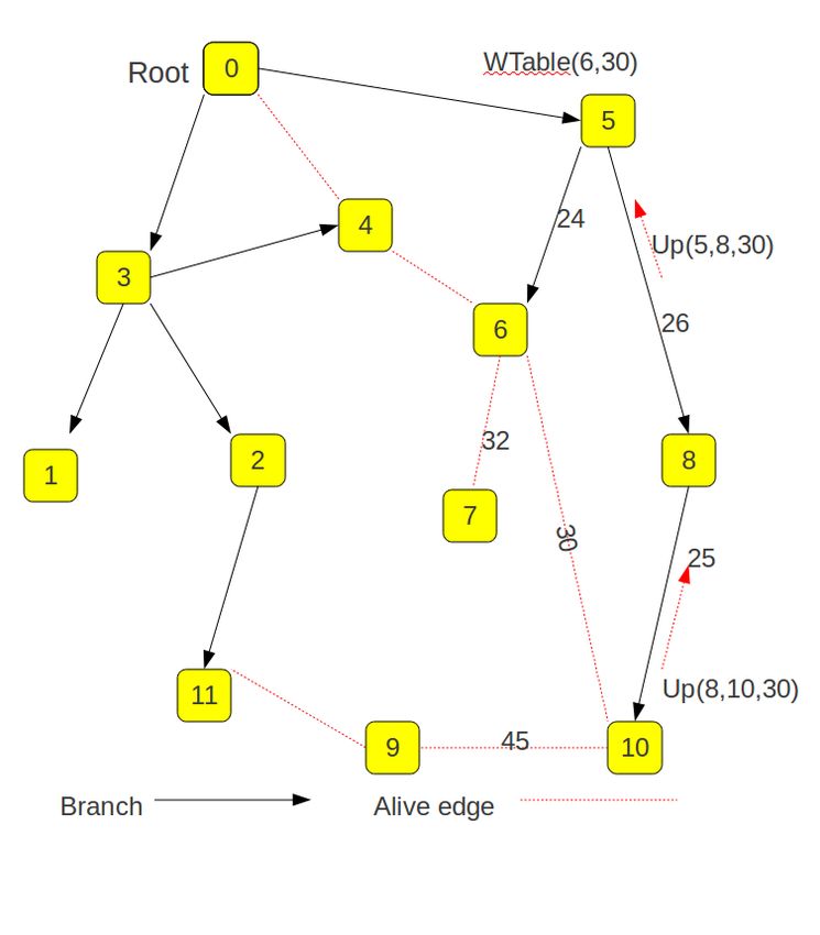
suitable additional information, namely facts WTable(y, m),
The asynchronous version of Netlog is used here. We
so that queries and invitations can be directed along the
assume a connected weighted graph, G = (V, E, w, R), where
suitable branch of the current spanning tree. Intuitively, a fact
V is the set of nodes, E is the set of Edges, the weight
WTable(y, m) stored on some node x of the spanning tree
w : E → R+, satisfies w(u, v) = w(v, u) for all edge (u, v)
is intended to indicate the weight of the outgoing edge of
in E, and R ∈ V a distinguished node called the root. In
smallest weight beyond y, when the edge (x, y) is on the
addition, we assume that w is injective. In other words, weights
spanning tree. A further subtle optimization is performed when
of different edges are distinct and then the MST is unique.
adding a new leaf to the spanning tree: no check is made on
The original algorithm [15], [16] starts from the root R and
the status (OnST or ¬OnST ) of its neighbors. Therefore,
constructs successive fragments of the MST, by adding to the
WTable(y, m) contains the weight of the MWAE (minimum
current fragment its minimal outgoing edge at each step. This
weight alive edge) below y, rather than the MWOE .
algorithm is easy to translate to centralized Netlog.
As for BFS, the spanning tree is represented by facts Definition 5 (dead, alive). An edge (a, b) such that a is in
OnST (a) and ST (a, b). Moreover, we define an intermediate OnST is either alive, dead, or a member of ST : it is initially
relation MWOE (x) to designate the minimal out-going weight alive (as soon as a becomes a member of OnST ) and becomesdead when a transmits to b an invitation to become a member
of OnST – the corresponding WTable entry at a is then
removed. Later, (a, b) will turn to ST if ¬OnST (b) or will
definitely remain dead if OnST (b), without this having any
significance with regard to values of MWAE.
Note that the same message is used for inviting a node b
to join the spanning tree and for querying the next MWAE
below b. This yields the following Netlog program.
MST-Prim-Dis
↓ OnST (loc)
Root(@loc)
↓ WTable(y, n) ← (6)
Weight(y, n)
↑ Down(loc, @loc, min(n))
Down(x, @loc, m) Node 5 first emitted an invitation Down to node 6; the
↑ Down(loc, @y, m) ← !WTable(y, m) (7) conflict appears in node 5 when receiving U p(5, 8, 30)
¬Weight(x, m) after node 10 joined the ST fragment, and is solved by
↓ OnST (loc) rule (13) which eventually removes alive edge 30.
Down(x, @loc, m)
↓ ST (x, loc) ¬ OnST (loc)
← (8) Figure 1. Fake invitation
↓ WTable(z, n) Weight(z, n)
↑ Up(@x, loc, min(n)) n 6= m
Rules (10) to (12) assume that the weight m carried by
Down(x, @loc, m)
↑ Up(@x, loc, dead) ← OnST (loc) (9) an arriving Up is not already stored in WTable. Rule (10)
Weight(x, m) guarantees that W T able stores a distinct weight, in order to
Up(@loc, y, m)
ensure uniqueness of the destination of Down in a future
↓ WTable(y, m) ← ¬WTable(_, m) (10) execution of rule (7). However, the distributed setting makes it
m 6= dead. possible for a MWAE to arrive from two different branches to
Up(@loc, y, m) the same node: this happens when, and only when, this edge
links two OnST nodes and has not yet been recognized as a
WTable(z, n)
↑ Up(@x, loc, min(m, n)) ← (11)
¬WTable(_, m)
dead edge (see Figure 1). The fake invitation rule (13) fixes
ST (x, loc) this issue, by enforcing the eventual triggering of rule (9) and
Up(@loc, y, m) appropriate cleaning.
WTable(z, n)
↑ Down(loc, @loc, min(m, n)) ← (12)
¬WTable(_, m)
B. Certification of Distributed Prim’s Algorithm
Root(loc)
Up(@loc, y, m)
This section presents the main ideas of the proof. Our goal
↑ Down(loc, @y, m) ← (13) is to verify that the program satisfies two properties: safety
WTable(_, m)
– each new joining edge is the minimal outgoing edge of the
Facts Down and Up are messages. After initialization of the current fragment, which means that the distributed ST relation
algorithm at the root (rule (6)) Down goes from the root (rules is consistent with the expected centralized view; and liveness
(6) and (12)) along the branch of the spanning tree leading to – the minimal weight outgoing edge of the current fragment
the MWAE (rule (7)), until it turns the selected alive edge will eventually be added to the ST. To this effect we prove
to an ST edge (rule (8)) or to a dead edge (rule (9)); by various technical lemmas. A key step states that WTable(d, w)
convention, the minimum of the empty set of weights is the records the minimal weight w among alive edges in branch d
special value dead assumed to be greater than any weight; and Up coming from d carries the minimal weight w among
then, if there is no outgoing edge from loc when triggering alive edges of branch d. As a corollary, Down generated at
rule (8), the aggregation min(n) evaluates to dead. Rule (9) the root contains the MWAE of the current fragment. Another
runs when discovering that the invited node links two OnST lemma states that rule (13) behaves as expected. Combining
nodes. Note that rule (7) deletes the relevant WTable entry them we get:
because the information contained there becomes unreliable. Theorem 1 (Safety). Each new joining edge is the minimal
Then, an Up message carrying the minimum weight alive outgoing edge of the current spanning tree.
edge (or dead, the maximum weight value, if no one exists) is
sent back to the root (rule (11)), restoring WTable (rule (10)) Additionally, we can prove a liveness property.
and, eventually, generating a new Down at the root (rule (12)). Theorem 2 (Liveness). The minimal weight outgoing edge of
Note that WTable is not restored when the corresponding the current fragment will eventually be added to the ST.
branch is dead. In rules (11) and (12), min(m, n) represents
the least value among m and the min-aggregation of all n Corollary 3 (Termination). All nodes will eventually belong
satisfying the body. to the spanning tree.C. Detailed Proofs Proof: Down is passed along WTable, which only exists
in OnST nodes by Lemma 4 (ii).
Lemma 4. (i) If a node x is a member of OnST , then
OnST (x) is stored on x. (ii) Any node which is not a member Lemma 10 (ST). (i) When a new ST (x, loc) is added, then
of OnST contains an empty WTable. (iii) Running rules (6) x is an OnST node and loc is a ¬OnST node; this happens
and (8) on some node creates of a new WTable on this node. only by triggering rule (8). (ii) The set of ST facts makes up
Proof: (i) and (iii) are easy inductive invariants, by a tree.
inspection of the rules; note that initially, no node is a member Proof: For (i), only rule (8) can add a fact ST (x, loc),
of OnST and all WTable are empty. (iii) is a consequence i.e., when a ¬OnST node loc receives Down from node x.
of (i) and (ii). Lemma 9 tells us that moreover x is an OnST node. (ii) is
an inductive invariant, using (i) when rule (8) is triggered.
Lemma 5. In any node, the facts stored in WTable contain
distinct values in their second argument. Lemma 11. Down generated in rule (13) carries the weight
Proof: Only rules (6), (8) and (10) may store values in of an edge connecting two OnST nodes.
WTable. For rules (6), (8) the third argument is a weight, Proof: Rule (13) is executed at node loc upon reception of
we then use the fact that all weights are distinct as well as an Up from branch y carrying some weight m already stored
Lemma 4 (iii). For rule (10), the conclusion follows from the in WTable for another branch x. By uniqueness of weights in
second literal of the body. the graph, and since ST is a tree by Lemma 10 (ii), m is the
weight of some alive edge (a, b), by Lemma (7)(A) for branch
Lemma 6. In any configuration there is at most one message y, and of the symmetric alive edge (b, a), by Lemma (7)(B)
among Down and Up. for branch x. By definition 5, a and b are then in OnST .
Proof: This is not difficult to check by chasing the rules
Proof of Theorem 1: By Lemma 10 (i), any edge (a, b)
of the program. Lemma 5 and rule (7) guarantee that only one
joining ST is an outgoing edge from the current fragment,
Down is sent along the suitable branch.
and its weight w is carried by a Down message. In addition,
Lemma 7. (A) WTable(d, w) records the minimal weight w this Down cannot have been generated by rule (13), because,
among all the alive edges of the branch d. (B) Up(x, d, w) from Lemma 11, b would be ¬OnST . This Down was then
coming from node d carries the minimal weight w among all generated by rule (12) and, by Corollary 8, w is the weight of
the alive edges of branch d. the minimal alive edge of the current tree. Altogether (a, b) is
Proof: (A) and (B) obviously hold in the initial configu- actually the MWOE of the current spanning tree.
ration. Now, assume (A) and (B) in a given configuration. Let Lemma 12. When a node receives Up with a non dead value
us first show that (A) holds in the next configuration obtained w, it stores w in WTable.
after a round. WTable could be changed in three possible Proof: Trivial from rule (10).
ways. (i) creation (rules (6) or (8)): for each neighbor d,
the corresponding branch starting contains just the edge to Lemma 13. When a node loc receives Down(x, loc, w) from
d, which is alive and stored in WTable according to rules node x and Weight(x, loc) 6= w (body of rule (7)), then at
(6) and (8), then (A) holds in the next configuration; (ii) node loc, WTable must contain an entry with value w.
deletion: if a node a passes Down to d using rule (7), the Proof: If x passes Down to loc, we know that, before
corresponding WTable entry for d is deleted at a and the Down is sent, there is a WTable entry with parameters loc
edge (a, d) is no longer alive, hence (A) holds in the next and w weight value stored at x. Since Weight(x, loc) 6= w,
configuration; (iii) updating: when node a receives Up from WTable(y, w) was generated by an Up coming from branch
node d by rule (10), Up carries the minimal weight m of loc, i.e., by rule (8), or (11), from Lemma 12, then it also
branch d by assumption (B) on the current configuration, and stored a WTable entry with value w at node loc. This entry
m is stored in WTable for branch d if m is not dead, ensuring could not be removed because rule (7) had no opportunity to
(A) in the next configuration. be enabled on node loc, as a consequence of Lemma 6.
Next let us show that (B) holds as well in the next con- Lemma 14 (run). While there is an alive edge in the graph,
figuration. Up is emitted from in two possible ways: (i) with there is exactly one message among Up and Down and the
a dead value in rule (9), indicating that there is no more program runs without deadlock.
alive edge; (ii) with the minimal weight w among alive edges Proof: In the initial configuration, exactly one Down mes-
below itself, by rules (8), and (11); using assumption (A) for sage is generated by rule (6). Then by inspection of the rules,
all OnST node from this node, we get that (B) holds in the Lemmas (6), (7) (A) and (10) (ii), we always have exactly one
next configuration. message Down or Up in the following configurations, except,
Corollary 8 (MWAE). The value w carried by a message at the root, when the WTable is empty, which means that the
Down(root, root, w) generated in rule (12) is actually the set of alive edges is empty by Lemma (7) (A). Now we need
MWAE of the current spanning tree. to prove that when a message Down or Up exists, there is no
deadlock (a rule can be triggered). This follows from (A) and
Lemma 9. Only an OnST node can pass a Down message. (B) below.(A) A message Down exists in three situations: (i) it is a Our experience on Prim’s algorithm is less advanced, since
newly generated message by rule (6), (12), or (13); triggering the Coq formalization has only been carried out on the model.
rule (6) or (12) immediately stores the value w carried by However, in this case, Netlog already turned out to be a
Down in the local WTable, while triggering (13) has the suitable framework for designing correctness proofs. The two
same effect by Lemma 12; then Down will be passed down to central characteristics of Netlog in this respect are its high
the right branch using rule (7). (ii) a node loc receives Down level of expression and its data-centric features.
from node x, and Weight(x, loc) 6= w; again, rule (7) can Our current Coq development contains about 7000 lines of
be applied from Lemma 13; (iii) a node loc receives Down Coq [17]: 1200 for the general model and common libraries,
from node x, and weight(x, y) = w (Down reaches the target and 5800 for the case studies about BFS and Prim’s algorithm.
edge); a rule among (8) and (9) is triggered, generating U p We estimate that completing the formalization in Coq of our
at the same time. proof of Prim’s algorithm would require about two months.
(B) From rules (8) and (9), we see that after a node passes Future work will include the study of GHS and other kinds of
Down to the suitable edge, it will receive Up from the same data-centric protocols.
edge. If a node receives Up with weight value w, either there
R EFERENCES
is already a WTable with the same w stored locally, then it
consumes Up and generates Down by rule (13); or it passes [1] Y. Deng, S. Grumbach, and J.-F. Monin, “A Framework for Verify-
ing Data-Centric Protocols,” in FMOODS/FORTE 2011, ser. LNCS,
Up to its parent along ST . When Root receives Up and gets R. Bruni and J. Dingel, Eds., vol. 6722. Reykjavik, Iceland: Springer,
a non-empty WTable, it triggers rule (12). June 6-9 2011, pp. 106–120.
[2] C. Kirkwood and M. Thomas, “Experiences with specification and
Proof of Theorem 2: Let us say that an oriented edge (a, b) verification in LOTOS: a report on two case studies,” in WIFT’95. IEEE
is outside when it is alive or when a is not OnST . From Computer Society, 1995, p. 159.
[3] F. Regensburger and A. Barnard, “Formal Verification of SDL Systems
definition 5, an edge is either outside, dead or in ST . When at the Siemens Mobile Phone Department,” in TACAS’98. Springer,
a Down message reaches a leaf b from node a, rule (8) 1998, pp. 439–455.
or (9) is triggered; new edges (b, x) may become alive if b [4] J.-C. Fernandez, H. Garavel, L. Mounier, A. Rasse, C. Rodriguez, and
J. Sifakis, “A toolbox for the verification of LOTOS programs,” in
becomes OnST , which does not change the cardinality of ICSE’92. ACM, 1992, pp. 246–259.
outside edges; at the same time (a, b) turns from alive to either [5] R. G. Gallager, P. A. Humblet, and P. M. Spira, “A Distributed Algorithm
dead or ST ; altogether, the number of outside edges decreases for Minimum-Weight Spanning Trees,” ACM Trans. Program. Lang.
Syst., vol. 5, no. 1, pp. 66–77, 1983.
by one. [6] J. L. Welch, L. Lamport, and N. Lynch, “A lattice-structured proof
Now, by Lemma 14, a configuration which contains alive of a minimum spanning,” in Proceedings of the seventh annual ACM
edges contains a message among Up and Down, and this Symposium on Principles of distributed computing, ser. PODC’88.
New York, NY, USA: ACM, 1988, pp. 28–43. [Online]. Available:
message propagates along ST , eventually reaching the root http://doi.acm.org/10.1145/62546.62552
(for Up) or a leaf (for Down) since ST is a tree by Lemma 10. [7] W. H. Hesselink, “The Verified Incremental Design of a Distributed
In both cases, a Down message is eventually generated and Spanning Tree Algorithm: Extended Abstract,” Formal Asp. Comput.,
vol. 11, no. 1, pp. 45–55, 1999.
reaches a leaf where the number of outside edges is decre- [8] Y. Moses and B. Shimony, “A New Proof of the GHS Minimum
mented. The theorem results from the finiteness of the initial Spanning Tree Algorithm,” in DISC, ser. Lecture Notes in Computer
number of outside edges. Science, S. Dolev, Ed., vol. 4167. Springer, 2006, pp. 120–135.
[9] J. S. Moore, “An acl2 proof of write invalidate cache coherence,” in CAV,
ser. Lecture Notes in Computer Science, A. J. Hu and M. Y. Vardi, Eds.,
V. C ONCLUSION vol. 1427. Springer, 1998, pp. 29–38.
[10] F. Verbeek and J. Schmaltz, “Formal specification of networks-on-
It is well-known that distributed algorithms may have very chips: Deadlock and evacuation.” in International Conference on Design
subtle behaviors, which make their design and proofs rather Automation and Test Europe (DATE’10). Dresden, Germany: IEEE,
March 2010.
delicate. Moreover, once a proof is done, we still have to [11] B. T. Loo, J. M. Hellerstein, I. Stoica, and R. Ramakrishnan, “Declar-
consider its maintenance. It is very easy to go from a cor- ative routing: extensible routing with declarative queries,” in ACM
rect system to a mistaken one through seemingly innocuous SIGCOMM’05, 2005.
[12] B. T. Loo, T. Condie, M. N. Garofalakis, D. E. Gay, J. M. Hellerstein,
changes and, in practice, implementations of correctly de- P. Maniatis, R. Ramakrishnan, T. Roscoe, and I. Stoica, “Declarative net-
signed protocols commonly introduce such modifications. working: language, execution and optimization,” in ACM SIGMOD’06,
The experience reported here supports the view that rule- 2006.
[13] C. Liu, Y. Mao, M. Oprea, P. Basu, and B. T. Loo, “A declarative
based languages such as Netlog provide a helpful level of perspective on adaptive manet routing,” in PRESTO’08. ACM, 2008,
abstraction not only for implementing data-centric distributed pp. 63–68.
algorithms, but also for reasoning effectively about them. This [14] S. Grumbach and F. Wang, “Netlog, a Rule-Based Language for Dis-
tributed Programming,” in PADL’10, ser. LNCS, vol. 5937, 2010, pp.
claim is seconded by our Coq formal model of Netlog which 88–103.
allows us to design and perform very accurate proofs. Our [15] V. Jarnìk, “O jistèm problému minimàlnìm [about a certain minimal
experience on BFS showed the robustness of a fully formalized problem],” Práce Moravské Přìrodovědecké Společnosti, vol. 6, pp. 57–
63, 1930, (in Czech).
case study with relation to two non-trivial modifications (in [16] R. C. Prim, “Shortest connection networks and some generalizations,”
that case: not of the algorithm itself, which is very short, but Bell System Technical Journal, vol. 36, pp. 1389–1401, 1957.
of the underlying model): overall, less than 5% of the code [17] M. Chen, Y. Deng, and J.-F. Monin, “Coq Script for Netlog Protocols,”
http://www-verimag.imag.fr/~monin/Proof/NetlogCoq/netlogcoq.tar.gz.
had to be changed in order to recover the desired results.You can also read