Assessing the Impact of Increased Effluent Discharge into Cape Cod Canal
←
→
Page content transcription
If your browser does not render page correctly, please read the page content below
Assessing the Impact of Increased Effluent Discharge into Cape Cod
                                Canal
J. Churchill, Dept. Phys. Oceanography, WHOI, Woods Hole, MA 02543 508‐289‐2807, jchurchill@whoi.edu
G. Cowles, SMAST, UMass Dartmouth, New Bedford, MA 02744 508‐910‐6397, gcowles@umassd.edu
J. Rheuban, WHOI, Dept. Mar. Chemistry, WHOI, Woods Hole, MA, 02543 508‐289‐3782, jrheuban@whoi.edu
                                              Final Report

1. Introduction

1a. Background
The Town of Wareham is considering a significant expansion of its wastewater treatment facility
(WWTF) that would enable it to serve additional neighborhoods in Bourne, Plymouth, and Wareham.
Currently, the treated effluent from the Wareham WWTF is discharged into the Agawam River, a shallow
(order 1‐m mean depth at high water) branch of the Wareham River. As part of the plan to expand its
WWTF, the Town of Wareham is considering relocating its effluent outfall to the western end of Cape
Cod Canal, at or near the site of the sewage outfall of the Massachusetts Maritime Academy (MMA;
Figure 1). This is deemed to be a more suitable location for effluent discharge than the Agawam River
due to the vigorous tidal flows, and attendant tidal flushing, in the canal. The volume of water passing
through the canal on a given flood or ebb tide is estimated to vary through the neap‐spring cycle over a
range of 14‐20 billion gallons (see the Appendix for details), which equates to a daily through‐canal flow
of roughly 56‐80 billion gallons (four times the volume passed on each ebb or flood tide).

As part of a feasibility study of the relocation plan, this project component sought to assess the effect
that increased effluent discharge through the MMA outfall would have on nutrient concentrations in the
vicinity (e.g., in upper Buzzards Bay, Cape Cod Canal and Cape Cod Bay). The fundamental question
addressed was whether or not the projected increase in effluent discharge associated with redirection
of the Wareham WWTF output would appreciably raise nutrient concentrations in critical
environments near MMA. Our assessment focused on the impact on total nitrogen (TN) concentrations
and was done in two parts. One part entailed using available data to estimate the present distribution
of TN in the aquatic environment near MMA. In the second, we used coupled hydrodynamic and plume‐
tracking models to estimate the additional TN contained in effluent discharged from the redirected
Wareham WWTF outfall. In examining the model results, we focused on the area very near (within a
few hundred meters) the MMA discharge and on four nearby regions deemed to be of particular
importance. These are: Buttermilk Bay, Butler Cove, Onset Bay and the area of Cape Cod Bay near the
eastern canal entrance (Figure 2).

                                                     1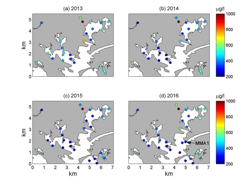
1b. Scenarios Considered
In modeling the effluent plume of the redirected Wareham WWTF discharge, we assumed that the
discharge would contain TN at a concentration of 3 mg l‐1. We considered two rates of volume
discharge: 3 and 10 million gallons per day (MGD) (Table 1). These roughly represent estimates of the
minimum and maximum volume outflow rates that would be required to accept redirected discharge
from the Wareham WWTF and from increased effluent production associated with planned expansion of
the sewer systems in Bourne, Wareham and Plymouth. As these daily volumes of effluent discharge are
much smaller than the roughly 56‐80 billion gallons of daily flow through the canal, one may expect
significant dilution of the effluent by the receiving waters in the canal.

The modeling system was also used to estimate the extent to which the present MMA effluent discharge
contributes to TN concentrations in the region near MMA. Currently, the MMA WWTF releases effluent
with relatively high TN concentrations (order 100 mg l‐1) at low flow rates (order 0.03 MGD) (Figure 3).
By contrast, the Wareham WWTF currently discharges effluent with much lower TN concentrations
(order 3 mg l‐1) at a considerably greater flow rate (of roughly 0.75 MGD). In modeling the effluent
plume of the current MMA discharge, we set the flow and TN concentration of the discharge to 0.03
MGD and 100 mg l‐1, respectively (Table 1). These values are representative of the average monthly
discharge for times of full student occupancy in MMA, which tend to be higher than the mean discharge
flow and TN concentration of months of low student occupancy (January, February, July and August)
(Figure 3).

1c. Report Outline
In the sections to follow, we first describe the data and analysis used to characterize the TN distributions
in our designated areas of interest. We then describe the hydrodynamic model used to simulate the
flows over the southern Massachusetts coastal zone. The operation of the model and verification of
model results are presented. Attention is then directed at the formulation and operation of the model
used to track effluent discharged from the MMA outfall. As will be more fully explained, the effluent
tracking is done using the velocities generated by the hydrodynamic model. Results of the effluent
tracking are then discussed with a focus on the extent to which the projected effluent outflow
associated with relocation of the Wareham WWTF discharge increases TN concentrations in the
designated areas of interest. We conclude in the final section with a summary of the findings.

2. Background Nutrient Fields
Two sources of data are used to estimate the background concentration of TN in our designated areas of
interest. TN concentrations in upper Buzzards Bay are derived from data collected through the Buzzards
Bay Coalition's (BBC’s) long‐term citizen‐science monitoring program. As part of this program, water
samples are collected by citizen volunteers over the summer months (principally in July and August)
during the last three hours of an outgoing tide. The samples are either filtered on site or after

                                                     2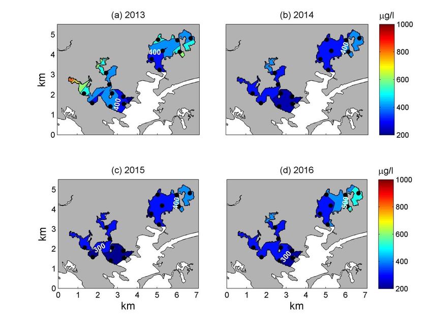
immediate transport to a laboratory. They are then kept on ice and in the dark while transported for
further analysis at the Marine Biological Laboratory. Inorganic nutrients, nitrate and nitrite, (NO3‐ and
NO2‐) are analyzed spectrophotometrically by automated Cd reduction (Johnson and Petty, 1983).
Ammonium (NH4+) is measured using the phenol hypochlorite method (Strickland and Parsons, 1972).
Total dissolved nitrogen (TDN; the sum of NO3‐ + NO2‐ + NH4+) is measured as nitrate following persulfate
digestion (D’Elia et al., 1977). Particulate organic nitrogen (PON) is measured by elemental analysis
(Sharp, 1974). The program’s methods are outlined in a Quality Assurance Project Plan that has been
approved by the Massachusetts Department of Environmental Protection and the U.S. Environmental
Protection Agency (Williams and Neill, 2014). Yearly averaged TN (sum of TDN and PON) concentrations
over 2013‐2016 are in the 200‐1000 μg l‐1 range within our designated areas of interest in upper
Buzzards Bay (Buttermilk Bay, Butler Cove, Onset Bay), with higher concentrations tending to occur in
the upper regions of these areas (Figures 4 and 5).

The data used to estimate the TN background concentration in Cape Cod Bay are from the Center for
Coastal Studies water quality monitoring program (www.capecodbay‐monitor.org), which since 2006
has collected water quality information from numerous stations in Nantucket and Vineyard Sounds and
in Cape Cod Bay. Three of the program’s stations are situated in the coastal zone within 10 km of the
eastern entrance to Cape Cod Bay (i.e., in our designated area of interest in Cape Cod Bay). The mean
(averaged over the last 10 years) TN concentration at these stations ranges between 211 and 384 μg l‐1
(Figure 6).

To estimate the background concentration in each designated area of interest, we averaged all TN
concentrations acquired over 2006‐2016 within each area (excluding small tributaries) (Figure 7). The
mean concentrations range from 275 (Cape Cod Bay) to 555 μg l‐1 (Butler Cove) (Table 2, Figure 8).

3. Hydrodynamic Model
As noted in the Introduction, the modeling component of this project was carried out in two parts. In
the first, model flows in the coastal region containing the MMA outfall and our designated areas of
interest were simulated with a high‐resolution hydrodynamic model. The second part entailed using the
modeled flow fields generated by the hydrodynamic model to simulate the transport and mixing of
effluent discharged at the MMA outfall. In this section, we present details of the hydrodynamic model.
Details of the plume tracking model are presented in Section 4.

3.1 Model Description

The hydrodynamic modeling was carried out using the Finite‐Volume Community Ocean Model (FVCOM:
Chen et al., 2006; Cowles, 2008), an open source model with over 4000 registered users that has been
applied in a wide array of coastal and open ocean studies. FVCOM operates by solving the equations of
motion on an unstructured grid, with elements that can be aligned with coastline and bathymetric
irregularities. To produce a 3‐dimensional solution, FVCOM employs a sigma‐coordinate system, in
which the vertical component of the model domain is divided into a fixed number of layers (20) that

                                                    3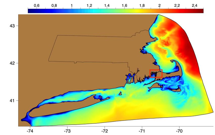
follow changes in model terrain. Layer thickness, for each of the 20 layers, is thus proportional to water
depth.

For this project, we utilized a regional FVCOM‐based model known as the Southeastern Massachusetts‐
FVCOM (SEMASS‐FVCOM), which includes the Massachusetts and Rhode Island coastal zones as well as
Long Island Sound (Figure 9). SEMASS‐FVCOM has been employed, and its results extensively evaluated,
by co‐PIs Cowles and Churchill for recent studies of tidal energy in the Massachusetts coastal zone
(Hakim et al., 2013; Cowles et al, 2017) and the dispersal of bay scallop larvae in Buzzards Bay (Liu et al.,
2015). Churchill and Cowles are currently using SEMASS‐FVCOM in two NOAA‐funded studies. One is
aimed at assessing the impact of climate change on the delivery of lobster larvae to suitable juvenile
habitat off of southern New England. The other is directed at quantifying the impact of municipal
sewage discharge on coastal acidification, focusing on effluent released by the towns of New Bedford,
Fairhaven and Wareham.

3.2 Grid Setup

To better resolve the hydrodynamic processes in the vicinity of the proposed wastewater outfall and our
designated areas of interest, the computational mesh of SEMASS‐FVCOM has been refined in Buzzards
Bay and Cape Cod Canal. The refined model grid contains 284,305 elements in the horizontal and 20
evenly spaced sigma‐layers in the vertical. The horizontal model‐grid resolution varies from 5 km over
the outer shelf to 50 m along the coastline of Buzzards Bay and within Cape Cod Canal (Figure 10).

The model bathymetry is interpolated from a composite dataset. The majority of the model domain is
encompassed by the 3‐arcsecond Gulf of Maine bathymetry product (Twomey and Signell, 2013) and the
1/3‐arcsecond Nantucket Inundation Digital Elevation Model (NOAA: Eakins et al., 2009). Data from a
directed sounding survey are used to specify the bathymetry of the Cape Cod Canal (USACE, 2011). The
coastal boundary is derived from a high‐resolution (1/2 arc‐second) product developed and distributed
by the Massachusetts Office of Coastal Zone Management.

3.3 Boundary Forcing

The model is driven at the open boundary by sea surface elevation constructed from the six primary
tidal constituents (M2, S2, N2, K1, O1 and M4). The phase and amplitude of these constituents and the
associated regional barotropic response have been extensively evaluated during the course of prior
work (Cowles et al., 2017). Values of the salinity and temperature of water flowing into the domain are
also set at the open boundary, and specified from a hindcast of a large scale Gulf of Maine / Southern
New England FVCOM‐GOM model developed by Dr. Changsheng Chen of U. Mass. Dartmouth (NeCOFS,
2017).

                                                      4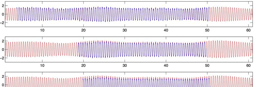
3.4 Surface Forcing

At the surface SEMASS‐FVCOM is driven by net heat flux and surface wind stress, which are also derived
from the regional 30‐year FVCOM‐GOM hindcast (NECOFS, 2017). The wind field in Buzzards Bay during
2015 (the year of our model run) displays a strong seasonality (Figure 11). The southwest sea breeze
dominates the Buzzards Bay wind field from late spring to early fall. By contrast, winds from late fall to
early spring are characterized by synoptic events with the strongest wind magnitudes directed from NW
and NE. These characteristics of the 2015 wind field are typical of the seasonal wind field in Buzzards
Bay (Liu et al., 2015). In addition to utilizing wind and heat flux data to force the model at the surface,
the model simulations also employ satellite‐derived sea surface temperature (SST) derived from the
NOAA 4 km‐resolution product. SST is assimilated into the model using a Newtonian relaxation
(nudging) approach, which adjusts the modeled SST to best match the observed SST.

3.5 Freshwater Input

Freshwater is input into the model domain at discrete points along the coastal boundary. The locations
of the freshwater entry points into Buzzards Bay are based on the watershed delineations of the
Buzzards Bay National Estuary Project, which established 32 watersheds draining into the bay.
Unfortunately, there is only one long‐term record of freshwater influx into the bay, from a gauge in the
Paskamansett River in Dartmouth (USGS 01105933). The freshwater flow from the other watersheds is
estimated by multiplying the gauged flow of Paskamansett River by the ratio of a given watershed’s area
to the area of the Paskamansett River watershed. Using this method we estimate that the average
freshwater discharge into the Bay in 2015 to be 21.3 m3 s‐1, which is 14% below the 20‐year annual
mean discharge of 25.0 m3 s‐1 (Figure 12). Inputs of freshwater from the major rivers outside the Bay
(Connecticut, Blackstone, Pawtuxet, Taunton, Neponset, and Charles) are included in the model and are
specified from hourly flow data recorded by USGS gauges (available from
https://waterdata.usgs.gov/nwis).

3.6 Execution and Data Archiving

The model was executed for the period Jan 1, 2015 to Jan 1, 2016 using a time step of two seconds. The
execution required 110,000 core‐hours of wall time on 2.6 GHz Intel Haswell Xeons. The two‐
dimensional fields of sea surface height and depth‐averaged velocity, and the three‐dimensional fields
of velocity, temperature, salinity, and the vertical turbulent eddy diffusivity and viscosity were archived
at hourly intervals into NetCDF format files. The total dataset (1.5 TB in size) is accessible through the
SMAST Thredds server at:
http://www.smast.umassd.edu:8080/thredds/catalog/buzzards/BBC_WW/catalog.html.

3.7 Model Verification

The model validation utilized long‐term observational records from upper Buzzards Bay. These included
velocity data from fixed ADCPs acquired as part of the NOAA CMIST program (Pruessner et al., 2007),
tidal constituents from the National Ocean Service database (NOS, 2016), and a long‐term bottom

                                                     5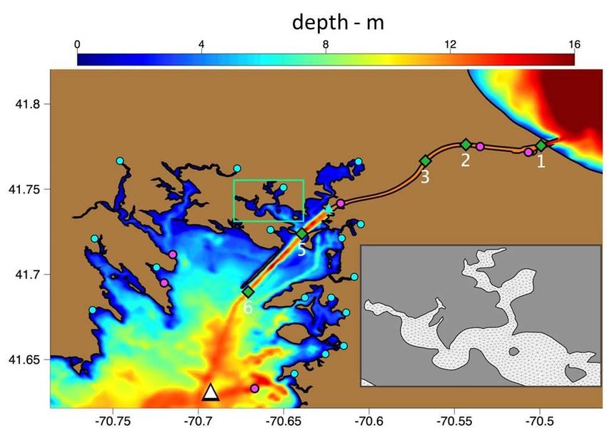
temperature record near Cleveland Ledge acquired by the Massachusetts Division of Marine Fisheries
(see Figure 10 for observation locations).

Sea Surface Elevation
The model simulation of sea surface elevation was compared with the sea surface records from the six
National Ocean Service tidal elevation stations (NOS, 2016) within upper Buzzards Bay and the Cape Cod
Canal (Figure 10). Surface elevation was extracted from the model hindcast at the grid points nearest
each station. Phase and amplitude of the principal regional tidal constituents (M2, S2, N2, K1, O1 and M4)
were then computed from the observed and modeled surface elevation time series using harmonic
analysis (T‐Tide, Pawlowicz et al., 2002).

The amplitude of the dominant M2 tide derived from the modeled sea levels is in close agreement, within
3 cm, of the observed M2 tidal amplitude at all NOS sites except at the Cape Cod Canal Railroad Bridge (5
cm) (Table 3). Within the domain of interest, the M2 phase rapidly varies due to the differences in the
tidal regimes of Cape Cod Bay (reflected by the Canal East station measurements; Table 3) and Buzzards
Bay (Nyes Neck). The amplitude and phase of the M2 tide in Cape Cod Bay differs from M2 tidal amplitude
and phase in Buzzards Bay by, respectively, a factor 2.4 and a lag of 3.5 hours. The model captures these
phase and amplitude differences as well as the variation of M2 phase and amplitude along the Canal (Table
3).

To quantify model skill, the observed and modeled tidal constituents were used to construct an annual
time series of tidal elevation at each NOS site. As illustrated by a comparison of modeled and observed
tidal records for July 2015 (Figure 13), the modeled tidal elevations are in close agreement with the
observations through the complete lunar cycle at all six stations. For skill we selected the root mean
square error (RMSE) and the dimensionless Willmott score (Willmott, 1981), which carries the value of 0
(no agreement) to 1 (perfect agreement). RMSE values for the six sites based on the annual time series
ranged from 3.4 to 8 cm; whereas Willmott scores ranged from 0.96 to 1.0.

Velocity
The model skill in simulating currents in upper Buzzards Bay was evaluated with water velocity
measurements acquired by five bottom‐mounted, upward‐looking ADCPs deployed for 1‐3 months in
2009 of as part of the NOAA CMIST program (Pruessner et al., 2007; see Figure 10 for locations). The
ADCP velocity data were archived at 6‐min intervals and extend vertically in 1.0‐m bins from 2.5 meters
above bottom to ~2 m below the surface.

To compare SEMASS‐FVCOM velocities with these measurements, the model was run for the duration of
the CMIST period (1 June 2009 ‐ 31 July 2009). The depth‐averaged modeled and measured velocities are
closely aligned in magnitude and phase, with the modeled velocities capturing the diurnal and spring‐
neap variation of the depth‐averaged velocities at all five sites (Figure 14).

The depth‐averaged velocity time series were decomposed into the principal tidal constituents (M2, S2,
N2, K1, O1 and M4) using the MATLAB routine T‐Tide (Pawlowicz et al., 2002). From these harmonic
constituents, annual time series of the tidal flows of both the observed and model‐computed currents
were reconstructed. Comparison of model‐ and data‐derived vertically averaged tidal flow magnitude at

                                                    6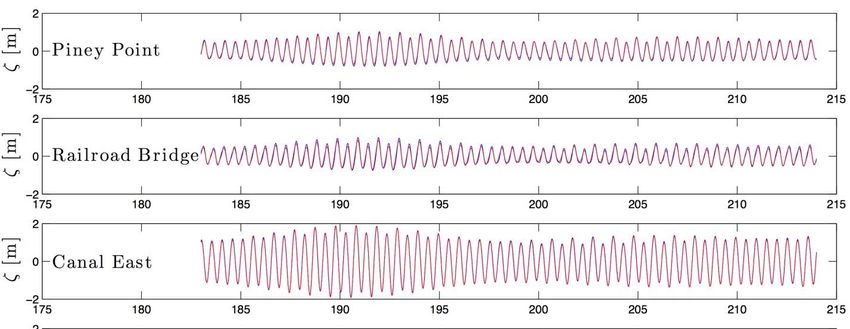
the five CMIST sites gave Willmott scores ranging from 0.96 to 0.99 and RMSE values from 5 to 25 cm s‐1
(Table 4).

The reconstructed time series were used to compare the model‐ and measurement‐derived vertical
profiles of mean velocity magnitude at each site. The vertical shear and magnitude of the measurement‐
and model‐derived velocities are in close agreement at CMIST‐1 (East entrance of the canal) and at CMIST‐
5 (just outside the West entrance of the Canal) and CMIST‐6 (Abiel’s Ledge) (Figure 15). The model under‐
predicts the mean velocity magnitude in the center of the Canal (by ~ 0.2 m s‐1), at CMIST‐2 and CMIST‐
3

At all sites, tidal ellipses computed from the measurement‐ and model‐derived reconstructed time series
of depth‐averaged currents are in close agreement in both orientation and magnitude (Figure 16).

Based on the above comparison, the model is judged capable of closely reproducing flows in Cape Cod
Canal and the upper portion of Buzzards Bay.

4. Plume‐Tracking Model
The plume tracking simulations were carried out using the high‐resolution three‐dimensional velocity
fields generated by the hydrodynamic model and focused on the transport and mixing of TN discharged
at the MMA outflow (i.e., effluent TN). We did not attempt to model the background concentration of
TN. Furthermore, the effluent TN was considered to be conservative. No attempt was made to account
for the transformation of effluent TN. As transformational processes would tend to extract effluent TN
from the water column (i.e., through transfer through the air‐water interface or through biological
uptake and transfer to the sediments), the modeled concentrations of effluent TN represent maximum
concentrations of TN released at the MMA outfall.

The plume tracking simulations operated by solving the diffusion‐advection equation in three
dimensions with a source term (applied at the outfall). Denoting the effluent TN concentration as CE,
the equation is expressed as

where: x, y and z are the east, north and vertical coordinates, respectively; t is time; u, v and w are the
east, north and vertical velocity components; KH and KV are the horizontal and vertical diffusivities; and
SS is the source of TN introduced at the outfall.

The solution of the above equation is carried out within model ‘tracer’ control volumes surrounding
each model node (Figure 17). Vertically, each control volume is divided into 20 evenly spaced layers,
corresponding to the hydrodynamic model’s sigma‐layers. Solving for the change in effluent TN
concentration (term A above) in each layer of each control volume entails determining the advective
fluxes (term B) of TN through the boundaries of the control volume layer (including through the layer’s
vertical boundaries), and the diffusive TN fluxes through the layer’s horizontal (term C) and vertical

                                                     7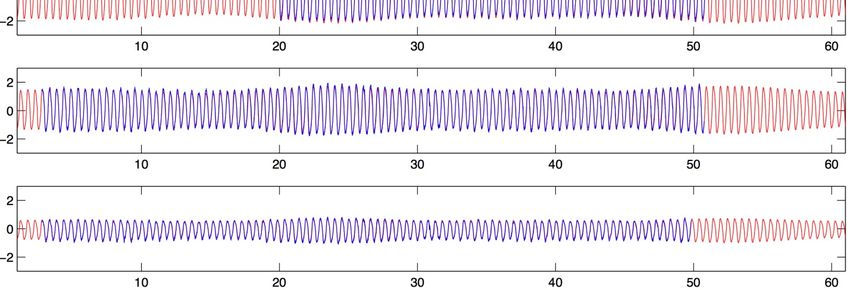
(term D) boundaries. The advective fluxes are determined with the velocities output from the
hydrodynamic model. In determining the horizontal diffusive fluxes, KH is set to a uniform value of 0.2
m2 s‐1. Values for KV are taken from the output of the hydrodynamic model (KV depends on the vertical
shear of the horizontal velocity) with a minimum value of 0.3 x10‐2 m2 s‐1 imposed.

The input of effluent TN (term E) occurs in the control volume encompassing the outfall (Figure 17) at a
rate (mass per unit time) of V*            , where             is the concentration of TN emerging from
the outfall and V is the volume rate of discharge (i.e., 10 MGD for scenario 3 in Table 1). It is assumed
that the discharged TN is initially mixed vertically and horizontally in the control volume containing the
outfall (which measures roughly 30x50 m). This is consistent with CTD measurements taken near the
outfall (by members of the project team and others) that show little vertical stratification in
temperature or salinity. It is assumed that all effluent TN passing through the model’s oceanic (open)
boundary (Figure 9) is lost to the system (i.e., does not return to the model domain). As the model
boundaries are far from our designated areas of interest, this boundary condition has no appreciable
effect on the modeled TN concentrations in these areas.

The model was executed in monthly increments for all of 2015. The final concentration field of each
month was used as the initial concentration field for the subsequent month. The model time step was
set at 20 s. In solving the equation for each time step, the velocities and KV values output by the
hydrodynamic model (at hourly intervals) were interpolated to center of each time step.

The model code was formulated (in MATLAB) by project team members Churchill, Cowles and Rheuban
for use in a MIT Sea Grant‐funded project aimed at quantifying the impact of municipal effluent
discharge on the carbonate system of coastal waters. As part of this project, the code has been subject
to considerable testing (i.e., by comparison of modeled and observed effluent concentration patterns).
In the simulations for this project, we checked for mass conservation (that the accumulated effluent TN
in the model domain equaled the amount discharged plus the amount lost at the open oceanic
boundary) and that the concentrations in each region matched the total mass in the region divided by
the region’s volume.

5. Estimates of Total Nitrogen Added by Effluent Discharge.
Results for the effluent tracking model are described below, focusing separately on the effluent TN
concentrations in the area of Cape Cod Canal very near the MMA outfall and on the effluent TN fields in
designated areas of interest further from the discharge. In discussing the results, the concentration of
effluent TN (i.e., the TN emanating from the discharge, which is separate from the ‘background’
concentration of TN in the receiving waters) is denoted at CE (see the above section). The vertical‐
average of CE is represented by , whereas the temporal average of  over some time period is
denoted as []T.

                                                     8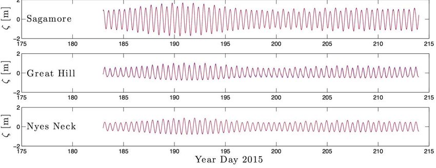
5.1 Added Total Nitrogen near the Discharge Site

Modeled values of []T reveal a tendency for the concentration of effluent TN to rapidly decline
moving away from the outfall (Figure 18). For example, []T determined for a 10 MGD discharge and
averaged over July declines from a maximum of roughly 7 μg l‐1 in the model cell containing the
discharge (which measures roughly 30 x 50 m) to less than 3 μg l‐1 in model cells roughly 100 m up‐canal
(to the NE) and down‐canal (to the SW) of the discharge (Figure 18c). The []T fields computed for a
projected 3 MGD discharge and for the current MMA discharge (Figure 18a,b) show a similar pattern
except with reduced []T (by a factor of 3.33 for the 3 MGD discharge and 10 for the current
discharge). Also apparent in all []T fields is a rapid decline in effluent TN concentration moving away
from the outfall in the cross‐canal direction. For example, in all monthly []T fields, the outfall cell
concentration is roughly four times higher than the concentration in the cell in the center of the canal
directly across from the outfall (e.g. Figure 18).

The rapid decline in  moving away from the outfall is reflected in the field of dilution ratio, defined
here as the ratio of the []T to the TN concentration released at the outfall (3 mg l‐1 for the projected
future discharge). Mathematically, the dilution ratio, D, is defined as

                                                             .

It should be noted that because a change in         will produce a corresponding change in []T ,
D does not depend on the discharged concentration (          ) and so is the same for all three
discharge scenarios considered (Table 1).

National shellfish sanitation regulations generally prohibit shellfish harvest within the area of a 1000:1
dilution from a WWTF outfall. D fields computed from []T of each simulation month show the
1000:1 contour tightly confined to the region near the discharge. In the most expansive monthly D field,
determined from the []T of July, the 1000:1 contour spans distances of roughly 45 and 300 m,
respectively, in the along‐ and across‐canal directions, and encompasses an area of approximately 0.13
km2 (Figure 19).

The rapid decline in effluent TN concentration moving away from the outfall is also apparent in the
instantaneous values  in the vicinity of the outfall (Figure 20). The modeled  recorded at the
outfall exhibits a wide variation linked with the strength of the tidal flow. The outfall TN concentrations
(averaged over the model cell (control volume) containing the discharge , Figure 17) are highest (order
50 μg l‐1) during slack tide conditions (at high and low water). During all other tidal phases,  at the
outfall is considerably smaller (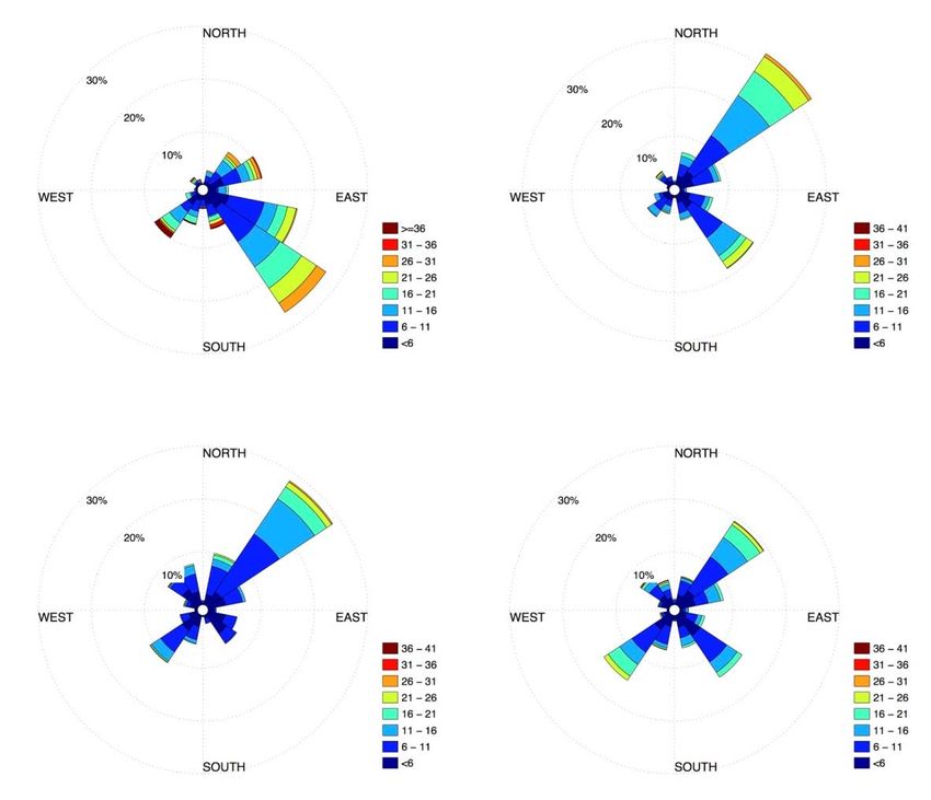
beginning of ebb (high tide), mid‐ebb (flow into the canal from Buzzards Bay), beginning of flood, mid‐
flood (flow into Buzzard Bay). During all tidal phases, there is very little vertical variation of  over
the transect, reflecting a high level of vertical mixing in the canal even near peak high and low water
levels. The highest  values (>8 μg l‐1) are seen at the beginning of ebb tide at the northern end of
the transect (adjacent to MMA). During mid‐ebb and mid‐flood,  is consistently low (
instantaneous values of  are even lower, not exceeding 1 μg l‐1 for a 10 MGD discharge (Figure 24d).
The model results indicate that CE tends to be vertically mixed throughout the water column in upper
Buzzards Bay, as illustrated by the contoured fields of CE along a line extending across the upper bay
(Figure 25).

To assess the impact of increased TN discharge on the TN concentrations in the designated areas of
importance, we compared the averaged measured TN in each area (which may be regarded as the
background TN concentration) (Table 2; Figures 7 and 8) to a similar average of the modeled‐estimate of
the TN added by the discharge. The averages of the modeled added‐TN shown here (Table 2, Figure 8)
were determined from modeled  fields from May‐September (roughly corresponding to the season
of the TN measurements in upper Buzzards Bay and Cape Cod Bay). The averages were taken over the
full extent of each designated areas (as indicated by the shading in Figure 7).

The results indicate that the projected increased discharge from the MMA facility should negligibly
impact TN concentrations in the designated areas of interest. For the maximum 10 MGD discharge, the
model‐estimated average of additional effluent‐TN within the areas of interest in upper Buzzards Bay
(Buttermilk Bay, Butler Cove, Onset Bay) is less than 0.5 % of the estimated background TN
concentration (Table 2, Figure 8). The impact of effluent‐TN is predicted to be even smaller in Cape Cod
Bay, where the averaged effluent TN concentrations are close to 0.1 % of the estimated background
concentration (Table 2, Figure 8).

The instantaneous values of  in each area of interest are consistently a small fraction of the
estimated background concentration,
of the Wareham WWTF outfall (3 mg l‐1 TN at 3‐10 MGD) will have little effect on the TN concentration
in the nearby aquatic environment. Among the notable model findings are:
The projected effluent discharge will increase the mean monthly TN concentration at the outfall
site by an of order 0.6 (3 MGD discharge) to 2 % (10 MGD discharge).
The instantaneous increase in TN concentration at the outfall due the discharged effluent is
greatest during periods of slack/near‐slack water, reaching a maximum of 5 % (3 MGD
discharge, not shown) to 17 % (10 MGD discharge) of the background TN concentration.
The concentration of TN discharged from the outfall declines rapidly going away from the
outfall. At ~275 m up‐ or down‐canal from the outfall, the predicted maximum (at slack water)
increase in TN concentration due to the discharge ranges from order 1 (3 MGD discharge) to 3 %
(10 MGD discharge) of the background concentration. The increase in mean TN concentration
at these distances from the outfall is order 0.2 (3 MGD discharge) to 0.7 % (10 MGD discharge)
of the background concentration.
The predicted increase in TN concentration within designated areas of interest in upper
Buzzards Bay (Buttermilk Bay, Butler Cove, Onset Bay) is no more than 1 % (10 MGD discharge)
of the background, while the predicted increase in TN concentration in Cape Cod Bay is no more
than 0.2 % (10 MGD discharge) of background concentration.
The region delineated by the 1000:1 dilution contour is roughly 45 m by 300 m around the
outfall and encompasses an area of approximately 0.13 km2
The rapid dilution of effluent predicted by the model reflects the flow conditions at the outfall. A
priori, rapid dilution of material discharged into Cape Cod Canal may be expected given the massive
volume of water passing through the canal on each tide (on the order of 20 billons gallons).
12References
Chen, C., Beardsley, R., Cowles, G. (2006). An unstructured-grid Finite-Volume Coastal Ocean Model
(FVCOM) System, Oceanography, 19 (1), 78–89.
Chen, C., Liu, H., Beardsley, R. C. (2003). An unstructured grid, finite-volume, three-dimensional,
primitive equations ocean model: application to coastal ocean and estuaries, Journal of
Atmospheric and Oceanic Technology, 20 (1), 159–186.
Cowles, G. W. (2008). Parallelization of the FVCOM coastal ocean model, International Journal of High
Performance Computing Applications, 22 (2), 177–193.
Cowles, G.W., Hakim, A., and Churchill, J. H., A comparison of numerical and analytical predictions of
the tidal stream power resource of Massachusetts, USA, Renewable Energy, in press.
D’Elia, C. F., and Steudler, P. A. (1977). Determination of total nitrogen in aqueous samples using
persulfate digestion, Limnology and Oceanography, 22, 760-764.
Eakins, B. W., Taylor, L. A., Carignan, K. S., Warnken, R. R., Lim, E., Medley, P. R. (2009). Digital
elevation model of Nantucket, Massachusetts: Procedures, data sources and analysis, National
Oceanic and Atmospheric Administration, National Environmental Satellite, Data, and
Information Service, National Geophysical Data Center, Marine Geology and Geophysics
Division.
Hakim, A. R., Cowles, G. W., and Churchill, J. H. (2013). The impact of tidal stream turbines on
circulation and sediment transport in Muskeget Channel, MA. Marine Technology Society
Journal, 47(4), 122-136. doi:10.4031/mtsj.47.4.14
Johnson, K. S., and Petty, R. L. (1983). Determination of nitrate and nitrite in seawater by flow injection
analysis. Limnology and Oceanography, 28, 1260 – 1266.
Liu, C., Cowles, G. W., Churchill, J. H., and Stokesbury, K. D. (2015). Connectivity of the bay scallop
(Argopecten irradians) in Buzzards Bay, Massachusetts, U.S.A. Fisheries Oceanography, 24(4),
364-382. doi:10.1111/fog.12114.
Liu, C., Cowles, G. W., Zemeckis, D. R., Cadrin, S. X., and Dean, M. J. (in press) Validation of a hidden
Markov model for the geolocation of Atlantic cod. Canadian Journal of Fisheries and Aquatic
Sciences.
NECOFS (2017) Northeast Coastal Ocean Forecasting System (NECOFS) Main Portal http:
//fvcom.smast.umassd.edu/necofs/. Accessed: 2017-05-20.
NOS Ocean Data Portal (2016) (Last Accessed: 2017-04-20). URL https://data.noaa.gov/dataset
Pawlowicz, R., Beardsley, B., Lentz, S. (2002). Classical tidal harmonic analysis including error
estimates in MATLAB using T_TIDE, Computers and Geosciences, 28 (8), 929–937.
Pruessner, A., Fanelli, P., Paternostro, C. (2007). C-MIST: An automated oceanographic data processing
software suite. in: Proceedings of the OCEANS 2007 Conference.
Sharp, J. H. (1974). Improved analysis for particulate organic carbon and nitrogen from seawater.
Limnology and Oceanography, 19, 984-989.
13Signell, R. (1987). Tide and wind-forced currents in Buzzards Bay, Massachusetts, M.S. Thesis,
Massachusetts Institute of Technology.
Strickland, J. D. H., and Parsons, T. R. (1972). Determination of ammonia. In A Practical Handbook of
Seawater Analysis, Fisheries Research Board of Canada, Bulletin 167 (Second Edition), 310
pages.
Twomey, E.R. and Signell, R.P. (2013). Construction of a 3-arcsecond digital elevation model for the
Gulf of Maine, U.S. Geological Survey Open-File Report 2011–1127, 24 pp,
https://pubs.usgs.gov/of/2011/1127/.
USACE, (2011). Cape Cod Canal Condition Survey, Tech. Rep. 11-1154, U.S. Army Corps of Engineers,
New England District, Concord, MA.
Williams, T., and Neill, C. (2014). Buzzards Bay Coalition Citizens’ Water Quality Monitoring Program,
“Baywatchers”, 5 Year Quality Assurance Project Plan.
Willmott, C. J. (1981). On the validation of models, Physical Geography, 2 (2), 184–194.
14Tables and Figures
Table 1. Modeled discharge scenarios.
Flow Rate (MGD) TN Conc. (mg l‐1)
Current MMA Discharge 0.03 100
Projected Minimum Flow Rate 3 3
Projected Maximum Flow Rate 10 3
Table 2. For four regions of particular interest, comparison of the averaged measured background
concentration of TN with the projected additional TN concentration due a 10 MGD effluent discharge
from the MMA outfall emerging into the canal with a TN concentration of 3 mg l‐1. See Figure 7 for
areas over which the averages were taken.
Measured Background* Modeled Effluent Addition
μg l‐1 μg l‐1
Ave. St. Dev Ave. St. Dev**
Buttermilk Bay 422 85 1.2 0.2
Butler Cove 555 92 1.4 0.4
Onset Bay 365 80 1.7 0.3
Cape Cod Bay 275 241 0.3 0.1
*The averaged background concentrations were computed from measurements taken over 2006‐2016
at the locations shown in Figure 7.
**The standard deviation of the modeled values was computed from the hourly values of the spatial
averages.Table 3. Phase and amplitude of the observed and modeled M2 tidal constituent at six tidal stations in upper Buzzards Bay and Cape Cod Canal. Columns 6 and 7 show the model skill in reproducing annual time series of tidal elevation at each site. Table 4. Skill assessment for the velocity computed from an annual time series constructed using the major axis of the constituents of the vertically averaged velocity field at 5 CMIST stations within the model domain (see Figure 10 for locations).
Figure 1. Satellite image of the Massachusetts Maritime Academy (MMA) facility with the MMA outfall
marked by a blue cross.
Figure 2. Nested view of the region of study. Indicated are areas of particular concern: Butler Cove,
Cape Cod Bay, Onset Bay and Buttermilk Bay. Also shown are points (sites CCB, ON, BC, BB, C1 and C2)
and transects [lines a‐b and c‐d in panel (c)] for which model data will be shown in subsequent figures.
The discharge location is marked in (b) and (c) by an arrow labeled ‘D’.
Figure 3. Monthly averaged volume discharge rate (top panel) and total N concentration (bottom
panel) in the effluent discharged from the MMA waste water treatment facility in 2015.
Figure 4. Scatter plots of yearly averaged TN concentration in (μg l‐1) in upper Buzzards Bay,
determined using TN concentrations from the Buzzards Bay Coalition's long‐term citizen‐science
monitoring program (see text). The site labeled ‘MMA1’ in (d) is the program’s sampling location closest
to the MMA sewage discharge.
Figure 5. Contours of yearly averaged TN concentration in (μg l‐1) in Buttermilk and Onset Bays,
determined using TN concentrations from the Buzzards Bay Coalition's long‐term citizen‐science
monitoring program (see text). The contours were determined with a two‐dimensional linear
interpolation algorithm using averaged concentrations from the stations marked by black dots.
Figure 6. Scatter plot of averaged TN concentration in (μg l‐1) in Cape Cod Bay, determined using TN
concentrations compiled by the Center for Coastal Studies (see text). The averaging period extended
over the full data set from each location (2006‐2016 for the northernmost station, 2006‐2010 for the
southern two stations).
Figure 7. Areas over which measured (at red points) and modeled (green shading) TN concentrations
were averaged.
Figure 8. Comparison of averaged measured TN concentration in areas of interest with the modeled
added TN concentration from an effluent discharge of 10 MGD. See Figure 7 for averaging areas and
Table 2 for concentration values.
Figure 9. SEMASS‐FVCOM model domain and bathymetry [log10(m)].
Figure 10. Portion of the FVCOM‐SEMASS domain in upper Buzzards Bay with bathymetry (m) (see Figure
9 for the full model domain). Also shown are measurement locations for CMIST upward‐looking ADCP
(numbered green diamonds), tidal harmonic elevation stations (magenta circles), and Mass Division of
Marine Fisheries long‐term bottom temperature record (white triangle) as well as the locations for point
sources of freshwater input to the upper bay (cyan circles) and approximate location of the proposed
outfall (cyan triangle). CMIST ADCPs are numbered East to West. Lower Figure Inset: Model grid in Onset
Bay.
Figure 11. Graphic representation of wind statistics of the modeled surface wind forcing at the
location of the proposed outfall. Magnitude is in knots. Upper Left: Jan 1 ‐ Mar 31, 2015. Upper
Right: Apr 1 ‐ June 30, 2015. Lower Left: Jul 1 ‐ Sep 30, 2015. Lower Right: Oct 1 ‐ Dec 31, 2015.
Figure 12. Total discharge (m3 s‐1) from all freshwater point sources to Buzzards Bay by year day.
Figure 13. Comparison of time series of tidal surface elevation [m] from measurements (blue) and
modeled (red) at the six NOS tidal stations in upper Buzzards Bay and Cape Cod Canal (Figure 10) during
July 2015. The model‐produced series is overlain over the observations and is often the only visible
series above.
Figure 14. Comparison of time series of depth‐averaged velocities (m s‐1) for the CMIST period (June‐
July, 2009). Time is days since June 1, 2009. The red line is the model‐computed value and the blue line
is the observed. The comparisons for CMIST Stations 1,2,3,5,6 (see Figure 10 for locations) are arranged
from top to bottom. Note that the observations cover different time periods. Model results are
shown for the first 61 days of 2009 and fully encompass each measured series.
Figure 15. Profiles of modeled (red solid lines) and observed (black lines with + symbols) annual mean
velocity magnitude at CMIST ADCP locations (Figure 10).
Figure 16. Tidal ellipses of model‐computed (red) and observed (blue) depth‐averaged velocity at
CMIST stations in upper Buzzards Bay. Shading represents bathymetry (m).
Figure 17. Borders of the tracer control volumes of the model grid in the area of the MMA
discharge outfall (labeled ‘D’ above). The control volume containing the outfall measures
roughly 50 by 30 m.
Figure 18. Vertically and temporally averaged concentrations (μg l‐1) of total nitrogen (TN)
contained in the discharged effluent (not including the background TN concentrations) for three
discharge scenarios (Table 1). The fields were computed from the model fields of July 2015.
Note that different color scales are used for each panel. Note also that the maximum
concentration in each panel [e.g., 7 μg l‐1 in panel (c), which is slightly larger than the scale
maximum to more clearly show the spatial variations of the TN field] is far lower than the
background TN concentrations shown in Figures 4‐5 (which are 200‐800 μg l‐1).
Figure 19. Contours of 500:1 and 1000:1 dilution ratios (ratios of discharged concentration to
vertically averaged modeled concentration) for a 10 MGD discharge. The field was determined
from modeled concentrations of July 2015 (month with the largest area encompassed by the
1000:1 dilution ratio contour). The area encompassed by the 1000:1 contour above is
approximately 0.13 km2.
Figure 20. Modeled vertically averaged effluent TN concentrations (μg l‐1) at three sites near
the western canal entrance (shown in Figure 3c) during late July (month with the highest near‐
discharge effluent TN concentrations). The fields were computed for a 10 MGD discharge.
Figure 21. Representative modeled concentration fields of effluent TN (μg l‐1) at the western
entrance to Cape Cod Canal (along line a‐b in Figure 3c) for four phases of the tide. The fields
were created with data from the tidal cycle with the maximum concentrations at the western
canal entrance during August, and were computed for a 10 MGD discharge.
Figure 22. Same as Figure 20 except showing modeled vertically averaged effluent TN
concentrations at three sites near the western canal entrance (shown in Figure 3c) as a function
of the percent of the background TN concentration (321 μg l‐1) at the western entrance.
Figure 23. Same as Figure 18 except showing a larger‐scale views of vertically averaged
concentrations (μg l‐1) of effluent TN for three discharge scenarios (Table 1). Note again, the
difference in scale in each panel and that the maximum concentration in each panel is far lower
than the background TN concentrations shown in Figures 4‐5.
Figure 24. Modeled vertically averaged effluent TN concentrations (for a 10 MGD discharge) at
sites in Cape Cod Bay and in Upper Buzzards Bay (shown in Figure 3a,b) during late July.
Figure 25. Same as Figure 21, except showing TN concentration fields (ug/l) in upper Buzzards
Bay (along line c‐d in Figure 3c).
Figure 26. Same as Figure 24 except showing the effluent TN concentrations at points in each
designated area (shown in Figure 3a,b) as a function of the percent of the measured TN
background concentration in each area (Figure 8 and Table 2).
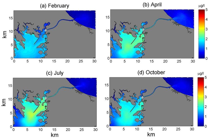
Figure 27. Modeled vertically averaged concentration fields (10 MGD discharge) of effluent TN
(μg l‐1) for four months. The discharge location is marked with a white ‘+’. Apparent is a
seasonal variation in the concentration fields. During winter and autumn (a and d), energetic
currents driven by predominantly down‐bay winds (Figure 11) produce maximum flushing of
discharged effluent from Buzzards Bay, resulting in relatively low effluent TN concentrations in
the upper bay. By contrast, modeled effluent TN concentrations in upper Buzzards Bay are
somewhat higher (though still two orders of magnitude lower than ambient/existing
conditions) during spring and summer (b and c), when wind forcing tends to be directed up the
bay (Figure 11).
Appendix: Estimating the Volume Transport through Cape Cod Canal on a Single Tide
To roughly estimate the volume of water transported through the canal on a given flood or ebb tide, we
may assume that the instantaneous volume flux, F, passing through a canal cross‐section at a given
time, t, is approximated by the product of the cross‐section’s area, A, and representative velocity, u(t),
flowing through the cross‐section. This may be expressed as:

                                                                   .

Further, assuming that A is a product of a representative canal width, L, and depth, D (ignoring changes
in D due to tidal excursions), gives:

                                                                       .

As a first approximation, we may assume that flow through the canal is dominated by the semidiurnal
tide with a period, P, of 12 hour 25 minutes, with u(t) expressed as:

                                                        sin                ,

where Ua is the peak tidal velocity. The instantaneous volume flux is then:

                                                         sin                   .

The total volume of water, V, transported through the canal on a given flood or ebb tide is then the
integral of the above over ½ the tidal period, i.e.
                                                    /
                                                               2
                                                        sin                        ,

which easily solves to:

                                                               .

To estimate V in the area of MMA, we may take L as 200 m (from Google Earth) and D as 12 m (from
USGS survey data). Based on NOAA tidal predictions of the canal current under the Cape Cod Railroad
Bridge, we may assign Ua values of 1.6 and 2.2 m s‐1, respectively, for neap and spring tides. The
resulting estimate of through‐canal volume transport is then 14 billion gallons for a neap tide (either
flood or ebb) and 20 billion gallons for a spring tide.

To form a second estimate of tidal volume transport through the canal, we use a record of water
velocity obtained from an Acoustic Doppler Current Profiler (ADCP) deployed in the canal as part NOAA’s
CMIST Program (see Section 3.7). The water depth and channel width at the deployment location (site 3
in Figure 10) are roughly 200 m (based on Google Earth) and 15 m (the ADCP deployment depth). Using
these values for L and D above, and taking the vertically averaged ADCP velocity for u(t), gives an
estimate of F(t). Integrating the F(t) time series gives a flood or ebb volume transport of roughly 16 billion gallons during a typical neap tide and 22 billion gallons during a typical spring tide. A third volume transport estimate may be determined from the velocities output by the project’s hydrodynamic model, SEMASS‐FVCOM (see Section 3). Using these velocities, we computed the transport through a section of the canal roughly situated beneath the Cape Cod Canal Railroad Bridge. In determining the volume flux [F(t) above], L and D were set to 200 m and 10 m, respectively, and u(t) was taken as an area‐average of the model‐output velocity along the section. Integrating the volume flux time series gives a flood or ebb volume transport of roughly 14 billion gallons during a typical neap tide and 20 billion gallons during a typical spring tide, consistent with the two estimates above. Based on these separate analyses, it may be assumed that the volume passing through the canal on a flood or ebb tide is order 14 billion gallons during ebb tides and order 20 billion gallons during spring tides.
You can also read