VENUS: Vertex-Centric Streamlined Graph Computation on a Single PC
←
→
Page content transcription
If your browser does not render page correctly, please read the page content below
VENUS: Vertex-Centric Streamlined Graph
                  Computation on a Single PC
                       Jiefeng Cheng1 , Qin Liu2 , Zhenguo Li1 , Wei Fan1 , John C.S. Lui2 , Cheng He1
                                                  1
                                                      Huawei Noah’s Ark Lab, Hong Kong
                              {cheng.jiefeng,li.zhenguo,david.fanwei,hecheng}@huawei.com
                                                  2
                                                      The Chinese University of Hong Kong
                                                      {qliu,cslui}@cse.cuhk.edu.hk

      Abstract—Recent studies show that disk-based graph compu-                Distributed computing systems such as Spark [13],
  tation on just a single PC can be as highly competitive as cluster-      Pregel [1], PEGASUS [5], and GraphLab [2] can handle
  based computing systems on large-scale problems. Inspired by             billion-scale graphs, but the cost of having and managing
  this remarkable progress, we develop VENUS, a disk-based graph           a large cluster is prohibitory for most users. On the other
  computation system which is able to handle billion-scale problems        hand, disk-based single machine graph computing systems
  efficiently on a commodity PC. VENUS adopts a novel computing
  architecture that features vertex-centric “streamlined” processing
                                                                           such as GraphChi [3], X-Stream [14], and TurboGraph [15]
  – the graph is sequentially loaded and the update functions              have shown great potential in big graph analytics. For example,
  are executed in parallel on the fly. VENUS deliberately avoids           running the PageRank algorithm on a Twitter graph of 1.5
  loading batch edge data by separating read-only structure data           billion edges, Spark needs 8.1 minutes with 50 machines (100
  from mutable vertex data on disk. Furthermore, it minimizes              CPUs) [16], while GraphChi only spends 13 minutes with just
  random IOs by caching vertex data in main memory. The                    a single MacMini of 8GB RAM and 256GB SSD drive; for
  streamlined processing is realized with efficient sequential scan        the belief propagation algorithm on a Web graph of 6.7 billion
  over massive structure data and fast feeding a large number              edges, PEGASUS takes 22 minutes with 100 machines [5],
  of update functions. Extensive evaluation on large real-world            while GraphChi uses 27 minutes on a single PC. These results
  and synthetic graphs has demonstrated the efficiency of VENUS.           suggest that disk-based graph computing on a single PC is not
  For example, VENUS takes just 8 minutes with hard disk for
  PageRank on the Twitter graph with 1.5 billion edges. In contrast,
                                                                           only highly competitive even compared to parallel processing
  Spark takes 8.1 minutes with 50 machines and 100 CPUs, and               over large clusters, but it is very affordable also.
  GraphChi takes 13 minutes using fast SSD drive.
                                                                               In general, graph computation is performed by iteratively
                                                                           executing a large number of update functions. The disk-based
                        I.   I NTRODUCTION                                 approach organizes the graph data into a number of shards
                                                                           on disk, so that each shard can fit in the main memory. Each
      We are living in a “big data” era due to the dramatic                shard contains all needed information for computing updates
  advance made in the ability to collect and generate data from            of a number of vertices. One iteration will execute all shards.
  various sensors, devices, and the Internet. Consider the Internet        A central issue is how to manage the computing states of
  data. The web pages indexed by Google were around one                    all shards to guarantee the correctness of processing, which
  million in 1998, but quickly reached one billion in 2000                 includes loading graph data from disk to main memory, and
  and have already exceeded one trillion in 2008. Facebook                 synchronizing intermediate results to disk so that the latest
  also achieved one billion users on October 4, 2012. It is                updates are visible to subsequent computation. Therefore, there
  of great interest to process, analyze, store, and understand             is a huge amount of data to be accessed per iteration, which
  these big datasets, in order to extract business value and               can result in extensive IOs and become a bottleneck of the
  derive new business model. However, researchers are facing               disk-based approach. This generates great interests in new
  significant challenges in processing these big datasets, due             architectures for efficient disk-based graph computation.
  to the difficulties in managing these data with our current
  methodologies or data mining software tools.                                 The seminal work for disk-based graph computation is
                                                                           the GraphChi system [3]. GraphChi organizes a graph into
      Graph computing over distributed or single multi-core plat-          a number of shards and processes each shard in turn. To
  form has emerged as a new framework for big data analytics,              execute a shard, the entire shard – its vertices and all of their
  and it draws intensive interests recently [1], [2], [3], [4], [5],       incoming and outgoing edges – must be loaded into memory
  [6], [7], [8], [9], [10], [11]. Notable systems include Pregel [1],      before processing. This constraint hinders the parallelism of
  GraphLab [2], and GraphChi [3]. They use a vertex-centric                computation and IO. In addition, after the execution, the
  computation model, in which the user just needs to provide a             updated vertex values need to be propagated to all the other
  simple update function to the system that is executed for each           shards in disk, which results in extensive IOs. The TurboGraph
  vertex in parallel [1], [2], [3]. These developments substantially       system [15] addresses these issues with a new computing
  advance our ability to analyze large-scale graph data, which             model, pin-and-sliding (PAS), and by using expensive SSD.
  cannot be efficiently handled by previous parallel abstractions          PAS aims to process incoming, partial graph data without de-
  such as MapReduce [12] due to sparse computation dependen-               lay, but it is applicable only to certain embarrassingly parallel
  cies and iterative operations common in graph computation [3].           algorithms. The X-Stream system [14] explores a different,

978-1-4799-7964-6/15/$31.00 © 2015 IEEE                             1131                                             ICDE Conference 2015
edge-centric processing (ECP) model. However, it is done by                                                                graph storage
writing the partial, intermediate results to disk for subsequent
processing, which doubles the sequential IOs while incurring                                                              structure value
                                                                                                     ...
                                                                           the input graph
additional computation cost and data loading overhead. Since
the ECP model uses very different APIs from previous vertex-                                       sharding
centric based system, the user need to re-implement many                offline preprocessing
graph algorithms on ECP which causes high development                   online graph computing
overhead. Moreover, certain important graph algorithms such
as community detection [17] cannot be implemented on the
ECP model (explained in Section IV-B).
   In this work, we present VENUS, a disk-based graph com-              big graph task think-like-a-          shard        buffer management
                                                                                       vertex program         execution
putation system that is able to handle billion-scale problems
very efficiently on a moderate PC. Our main contributions are
summarized as follows.                                                                   Fig. 1.   The VENUS Architecture

A novel computing model. VENUS supports vertex-centric
computation with streamlined processing. We propose a novel            experiments look into the key performance factors to all disk-
graph storage scheme which allows to stream in the graph data          based systems including computational time, the effectiveness
while performing computation. The streamlined processing can           of main memory utilization, the amount of data read and write,
exploit the large sequential bandwidth of a disk as much as            and the number of shards. And we found that VENUS is up
possible and parallelize computation and disk IO at the same           to 3x faster than GraphChi and X-Stream, two state-of-the-art
time. Particularly, the vertex values are cached in a buffer in        disk-based systems.
order to minimize random IOs, which is much more desirable                 The rest of the paper is organized as follows. Section II
in disk-based graph computation where the cost of disk IO is           gives an overview of our VENUS system, which includes a
often a bottleneck. Our system also significantly reduces the          disk-based architecture, graph organization and storage, and an
amount of data to be accessed, generates less shards than the          external computing model. Section III presents algorithms to
existing scheme [3], and effectively utilizes large main memory        substantialize our processing pipeline. We extensively evaluate
with a provable performance guarantee.                                 VENUS in Section IV. Section V reviews more related work.
                                                                       Section VI concludes the paper.
Two new IO-friendly algorithms. We propose two IO-
friendly algorithms to support efficient streamlined processing.                             II.   S YSTEM OVERVIEW
In managing the computing states of all shards, the first
algorithm stores vertex values of each shard into different                VENUS is based on a new disk-based graph computing
files for fast retrieval during the execution. It is necessary to      architecture, which supports a novel graph computing model:
update on all such files timely once the execution of each             vertex-centric streamlined processing (VSP) such that the
shard is finished. The second algorithm applies merge-join to          graph is sequentially loaded and the update functions are
construct all vertex values on the fly. Our two algorithms adapt       executed in parallel on the fly. To support the VSP model,
to memory scaling with less sharding overhead, and smoothly            we propose a graph storage scheme and an external graph
turn into the in-memory mode when the main memory can                  computing model that coordinates the graph computation and
hold all vertex values.                                                with CPU, memory and disk access. By working together,
                                                                       the system significantly reduces the amount of data to be
A new analysis method. We analyze the performance of our               accessed, generates a smaller number of shards than the
vertex-centric streamlined processing computation model and            existing scheme [3], and effectively utilizes large main memory
other models, by measuring the amount of data transferred              with provable performance guarantee.
between disk and main memory per iteration. We show that
VENUS reads (writes) significantly less amount of data from            A. Architecture Overview
(to) disk than other existing models including GraphChi. Based
                                                                           The input is modeled as a directed graph G = (V, E),
on this measurement, we further find that the performance of
                                                                       where V is a set of vertices and E is a set of edges. Like
VENUS improves gradually as the available memory increases,
                                                                       existing work [18], [19], the user can assign a mutable vertex
till an in-memory model is emerged where the least overhead is
                                                                       value to each vertex and define an arbitrary read-only edge
achieved; in contrast, existing approaches just switch between
                                                                       value on each edge. Note that this does not result in any loss of
the in-memory model and the disk-based model, where the
                                                                       expressiveness, since mutable data associated with edge (u, v)
performance can be radically different. The purpose of this
                                                                       can be stored in vertex u. Let (u, v) be a directed edge from
new analysis method is to clarify the essential factors for good
                                                                       node u to node v. Node u is called an in-neighbor of v, and v
performance instead of a thorough comparison of different
                                                                       an out-neighbor of u. (u, v) is called an in-edge of v and an
systems. Moreover, it opens a new way to evaluate disk-based
                                                                       out-edge of u, and u and v are called the source and destination
systems theoretically.
                                                                       of edge (u, v) respectively.
Extensive experiments. We did extensive experiments using                 Most graph tasks are iterative and vertex-centric in nature,
both large-scale real-world graphs and large-scale synthetic           and any update of a vertex value in each iteration usually in-
graphs to validate the performance of our approach. Our                volves only its in-neighbors’ values. Once a vertex is updated,

                                                                1132
6
the value table 8
7
v-shard 1
shard shard shard 5
... the structure table
9
4
Fig. 2. Vertex-Centric Streamlined Processing
2
3
it will trigger the updates of its out-neighbors. This dynamic
continues until convergence or certain conditions are met. The Fig. 3. Example Graph
disk-based approach organizes the graph data into a number of
shards on disk, so that each shard can fit in the main memory.
Each shard contains all needed information for computing the v-shard corresponding to the same vertex interval make
updates of a number of vertices. One iteration will execute a full shard. To illustrate the concepts of shard, g-shard, and
all shards. Hence there is a huge amount of disk data to be v-shard, consider the graph as shown in Fig. 3. Suppose the
accessed per iteration, which may result in extensive IOs and vertices are divided into three intervals: I1 = [1, 3], I2 = [4, 6],
become a bottleneck of the disk-based approach. Therefore, and I3 = [7, 9]. Then, the resulting shards, including g-shards
a disk-based graph computing system needs to manage the and v-shards, are listed in Table I.
storage and the use of memory and CPU in an intelligent way In practice, all g-shards are further concatenated to form the
to minimize the amount of disk data to be accessed. structure table, i.e., a stream of structure records (Fig. 2). Such
VENUS, its architecture depicted in Fig. 1, makes use a design allows executing vertex update on the fly, and is cru-
of a novel management scheme of disk storage and the cial for VSP. Using this structure, we do not need to load the
main memory, in order to support vertex-centric streamlined whole subgraph of vertices in each interval before execution
processing. VENUS decomposes each task into two stages: (1) as in GraphChi [3]. Observing that more shards usually incur
offline preprocessing and (2) online computing. The offline more IOs, VENUS aims to generate as few number of shards
preprocessing constructs the graph storage, while the online as possible. To this end, a large interval is preferred provided
computing manages the interaction between CPU, memory, that the associated v-shard can be loaded completely into the
and disk. main memory, and there is no size constraint on the g-shard.
Once the vertex values of vertices in v-shard is loaded and
B. Vertex-Centric Streamlined Processing then held in the main memory, VENUS can readily execute
the update functions of all vertex with only “one sequential
VENUS enables vertex-centric streamlined processing scan” over the structure table of the g-shard. We will discuss
(VSP) on our storage system, which is crucial in fast loading how to load and update vertex values for vertices in each v-
of graph data and rapid parallel execution of update functions. shard in Section III.
As we will show later, it has a superior performance with much
less data transfer overhead. Furthermore, it is more effective in Graph storage. We propose a new graph storage that aims
main memory utilization, as compared with other schemes. We to reduce the amount of data to be accessed. Recall that
will elaborate on this in Section II-C. To support streamlined the graph data consists of two parts, the read-only structure
processing, we propose a new graph sharding method, a new records, called structure data, and the mutable vertex values,
graph storage scheme, and a novel external graph computing called value data. We observe that in one complete iteration,
model. Let us now provide a brief overview of our sharding, the entire structure data need to be scanned once and only
storage, and external graph computing model. once, while the value data usually need to be accessed multiple
times as a vertex value is involved in each update of its out-
Graph sharding. Suppose the graph is too big to fit in the neighbors. This suggests us to organize the structure data as
main memory. Then how it is organized on disk will affect consecutive pages, and it is separated from the value data. As
how it will be accessed and processed afterwards. VENUS such, the access of the massive volume structure data can be
splits the vertices set V into P disjoint intervals. Each interval done highly efficiently with one sequential scan (sequential
defines a g-shard and a v-shard, as follows. The g-shard stores IOs). Specifically, we employ an operating system file, called
all the edges (and the associated attributes) with destinations the structure table which is optimized for sequential scan, to
in that interval. The v-shard contains all vertices in the g- store the structure data.
shard which includes the source and destination of each edge.
Edges in each g-shard are ordered by destination, where the Note that the updates and repeated reads over the value
in-edges (and their associated read-only attributes) of a vertex data can result in extensive random IOs. To cope with this,
are stored consecutively as a structure record. There are |V | VENUS deliberately avoids storing a significant amount of
structure records in total for the whole graph. The g-shard and structure data into main memory as compared with the existing
1133TABLE I TABLE III
S HARDING E XAMPLE : VENUS N OTATIONS
Interval I1 = [1, 3] I2 = [4, 6] I3 = [7, 9] Notation Definition
v-shard I1 ∪ {4, 6, 8, 9} I2 ∪ {1, 2, 7, 9} I3 ∪ {1, 2, 5, 6} n, m n = |V |, m = |E|
gs(I) g-shard of interval I
g-shard 2,4,6,8 → 1 1,6,9 → 4 1,5,9 → 7
vs(I) v-shard of interval I
4,6,9 → 2 1,2,6,7 → 5 6,7,9 → 8
S(I) {u 6∈ I|(u, v) ∈ gs(I)}
2,4 → 3 1,2,7,9 → 6 1,2 → 9 P
δ δ= I |S(I)|/m
S(I) 4 1 1 P number of shards
6 2 2 M size of RAM
8 7 5 C size of a vertex value record
9 9 6 D size of one edge field within a structure record
B size of a disk block that requires unit IO to access it
TABLE II
S HARDING E XAMPLE : G RAPH C HI
shard of I1 into the main memory. Then we load the g-shard
Interval I1 = [1, 2] I2 = [3, 5] I3 = [6, 7] I4 = [8, 9] in a streaming fashion from disk. As soon as we are done
loading the in-edges of vertex 1 (which include (2, 1), (4, 1),
Shard 2 → 1 1 → 4,5 1 → 6,7 1 → 9
(6, 1), and (8, 1)), we can perform the value update on vertex
4 → 1,2 2 → 3,5 2 → 6 2 → 9
1, and at the same time, we load the in-edges of vertices
6 → 1,2 4 → 3 5 → 7 6 → 8
8 → 1 6 → 4,5 7 → 6 7 → 8
2 and 3 in parallel. In contrast, to perform computation on
9 → 2 7 → 5 5 → 6,7 9 → 8
the first interval, GraphChi needs to load all related edges
9 → 4 (shaded edges in the table), which include all the in-edges and
out-edges for the interval. This means that for processing the
same interval, GraphChi requires more memory than VENUS.
So under the same memory constraint, GraphChi needs more
system GraphChi [3] and instead caches value data in main shards. More critically, because all in-edge and out-edges
memory as much as possible. VENUS stores the value data must be loaded before computation starts, GraphChi cannot
in a disk table, which we call the value table. The value parallelize IO operations and computations like VENUS.
table is implemented as a number of consecutive disk pages,
containing the |V | fixed length value records, each per vertex. C. Analysis
For simplicity of presentation, we assume all value records
are arranged in ascending order (in terms of vertex ID). Our We now compare our proposed VSP model with two pop-
key observation is that, for most graph algorithms, the mutable ular single-PC graph computing models: the parallel sliding
value on a directed edge (u, v) can be computed based on the windows model (PSW) of GraphChi [3] and the edge-centric
mutable value of vertex u and the read-only attribute on edge processing model (ECP) of X-Stream [14]. Specifically, we
(u, v). Consequently, we can represent all mutable values of look at three evaluation criteria: 1) the amount of data trans-
the out-edges of vertex u by a fixed-length mutable value on ferred between disk and main memory per iteration; 2) the
vertex u. number of shards; and 3) adaptation to large memory.
There are strong reasons to develop our analysis based
External computing model. Given the above description of on the first criterion, i.e., the amount of data transfer: (i) it
graph sharding and storage, we are ready to present our graph is fundamental and applicable for various types of storage
computing model which processes the incoming stream of systems, including magnetic disk or solid-state disk (SSD),
structure records on the fly. Each incoming structure record and various types of memory hierarchy including on-board
is passed for execution as the structure table is loaded se- cache/RAM and RAM/disk; (ii) it can be used to derive
quentially. A higher execution manager is deployed to start IO complexity as in Section III-C, which can be based on
new threads to execute new structure records in parallel, when accessing that certain amount of data with block device; and
possible. A structure record is removed from main memory (iii) it helps us to examine other criteria, including the number
immediately after its execution, so as to make room for next of shards and large memory adaption. We summarize the
processing. On the other hand, the required vertex values of the results in Table IV, and show the details of our analysis
active shard are obtained based on v-shard, and are buffered below. Note that the second criterion is related closely to IO
in main memory throughout the execution of that shard. As complexity, and the third criterion examines the utilization of
a result, the repeated access of the same vertex value can be memory.
done in the buffer even for multiple shards. We illustrate the
above computing process in Fig. 2. For easy reference, we list the notation in Table III. For our
VSP model, V is split into P disjoint intervals. Each interval
We use the graph in Fig. 3 to illustrate and compare the I has a g-shard and a v-shard. A g-shard is defined as
processing pipelines of VENUS and GraphChi. The sharding
structures of VENUS are shown in Table I, and those for gs(I) = {(u, v)|v ∈ I},
GraphChi are in Table II where the number of shards is and a v-shard is defined as
assumed to be 4 to reflect the fact that GraphChi usually uses
more shards than VENUS. To begin, VENUS first loads v- vs(I) = {u|(u, v) ∈ gs(I) ∨ (v, u) ∈ gs(I)}.
1134Note that vs(I) can be split into two disjoint sets I and S(I), we will show that the smaller of the number of shards, the
where S(I) = {u 6∈ I|(u, v) ∈ gs(I)}. We have lower of IO complexity.
X X
|S(I)| ≤ |gs(I)| = m. Adaptation to large memory. As analyzed above, for our
I I VSP model, the size of data needed to read in one iteration
Let δ be a scalar such that is C(n + δm) + Dm. So one way to improve performance is
X to decrease δ. Here we show that δ does decrease as the size
|S(I)| = δm, where 0 ≤ δ ≤ 1. of available memory increases, which implies that VENUS
I can exploit the main memory effectively. Suppose the memory
It can be seen that size is M , and the vertex set V is split into P intervals
PPi ) ≤ M for i = 1, . . . , P . Then,
I1 , I2 , . . . , IP , where vs(I
X X X
|vs(I)| = |S(I)| + |I| = δm + n. by definition, δm = i=1 |S(Ii )|. Now, consider a larger
I I I memory size M 0 such that M 0 ≥ |vs(I1 )| + |vs(I2 )| ≥ M .
Let C be the size of a vertex value record, and let D be the Under the memory size M 0 , we can merge interval I1 and
size of one edge field within a structure record. We use B to I2 into It , because |vs(ItP )| ≤ |vs(I1 )| + |vs(I2 )| ≤ M 0 .
P
denote the size of a disk block that requires unit IO to access Suppose δ 0 m = |S(It )| + i=3 |S(Ii )|. By the definition of
it. According to [14], B equals to 16MB for hard disk and S(I), it can be shown that S(It ) ⊆ S(I1 ) ∪ S(I2 ), and thus
1MB for SSD. |S(It )| ≤ |S(I1 )| + |S(I2 )|. Therefore we have δ 0 ≤ δ, which
means as M increases, δ becomes smaller. When M ≥ Cn,
Data transfer. For each iteration, VENUS loads all g-shards we have P = 1 where δ = 0. In such a single shard case, the
and v-shards from disk, which needs Dm and C(n+δm) data data size of read reaches the lower bound Cn + Dm.
read in total. When the computation is done, VENUS writes
v-shards back to disk which incurs Cn data write. Note that III. A LGORITHM
g-shards are read-only.
In this section, we discuss the full embodiment of our
Unlike VENUS where each vertex can access the values of
vertex-centric streamlined processing model, to describe the
its neighbors through v-shard, GraphChi accesses such values
details of our graph storage design, the online computing
from the edges. So the data size of each edge is (C + D). For
state management, and the main memory usage. It consists
each iteration, GraphChi processes one shard at a time. The
of two IO-friendly algorithms with different flavor and IO
processing of each shard is split into three steps: (1) loading
complexity in implementing the processing of Section II. Note
a subgraph from disk; (2) updating the vertices and edges;
that the IO results here are consistent with the data transfer size
(3) writing the updated values to disk. In steps 1 and 3, each
results in Section II because the results here are obtained with
vertex will be loaded and written once which incurs Cn data
optimization specialized for disk-based processing to transfer
read and write. For edges data, in the worst case, each edge is
the same amount of data. Since the computation is always
accessed twice (once in each direction) in step 1 which incurs
centered on an active shard, the online computing state mainly
2(C + D)m data read. If the computation updates edges in
consists of the v-shard values that belong to the active shard.
both directions in step 2, the size of data write of edges in
step 3 is also 2(C + D)m. So the data read and write in total Our first algorithm materializes all v-shard values in each
are both Cn + 2(C + D)m. shard, which supports fast retrieval during the online com-
puting. However, in-time view update on all such views is
In the disk-based engine of X-Stream, one iteration is
necessary once the execution of each shard is finished. We
divided into (1) merged scatter/shuffle phase and (2) gathering
employ an efficient scheme to exploit the data locality in all
phase. In phase 1, X-Stream loads all vertex value data and
materialized views. And this scheme shares a similar spirit
edge data, and for each edge it writes an update to disk. Since
with the parallel sliding window of [3], with quadratic IO
updates are used to propagate values passed from neighbors,
performance to P , namely the number of shards. In order
we suppose the size of an update is C. So for phase 1, the size
to avoid the overhead of view maintenance at run time, our
of read is Cn + Dm and the size of write is Cm. In phase 2,
second algorithm applies “merge-join” to construct all v-
X-Stream loads all updates and update each vertex, so the size
shard values on-the-fly, and updates the active shard only. The
of data read is Cm and the size of write is Cn. So for one
second algorithm has an IO complexity linear to P . Finally,
full pass over the graph, the size of read is Cn + (C + D)m
as the RAM becomes large, the two algorithms adapt to the
and the size of write is Cn + Cm in total.
memory scaling with less sharding overhead, and finally the
Number of shards. For interval I, VENUS only loads the two algorithms automatically work in the in-memory mode to
v-shard vs(I) into memory and the g-shard gs(I) is loaded in seamlessly integrate the case when the main memory can hold
a streaming fashion. So the number of shards is determined all vertex values.
by the total size of v-shards and we have P = C(n+δm)
M . In
contrast, GraphChi loads both vertex value data and edge data A. Physical Design And The Basic Procedure
for each interval, so the number of shards P in GraphChi is
Cn+2(C+D)m
. In X-Stream, edges data are also loaded in a The tables. The value table is implemented as a number
M
of consecutive disk pages, containing |V | fixed-length value
streaming fashion, so the number of intervals is P = Cn
M . records, each per vertex. For the ease of presentation, we
We can see that the number of shards constructed in assume all value records are arranged in the ascending order
VENUS is always smaller than that in GraphChi. In Section III, of their IDs in the table. For an arbitrary vertex v, the disk
1135TABLE IV
C OMPARISON OF DATA TRANSFERRED BETWEEN SINGLE -PC GRAPH COMPUTING SYSTEMS
category PSW ECP VSP
Data size (read) Cn + 2(C + D)m Cn + (C + D)m C(n + δm) + Dm
Data size (write) Cn + 2(C + D)m Cn + Cm Cn
Cn+2(C+D)m Cn C(n+δm)
No. of shard M M M
Procedure ExecuteVertex(v, R(v), VB, I) Algorithm 1: Execute One Iteration with Views
input : vertex v, structure record R(v), value buffer VB,
1 let I be the first interval;
and interval I.
2 load view(I) into the map of VB;
output: The updated record of v in the value table.
3 foreach R(v) in the structure table do
1 foreach s ∈ R(v) do 4 if v 6∈ I then
2 let Q be the b NsB c-th page of the value table; 5 foreach internal J 6= I do
3 if s ∈ I ∧ Q 6∈ V B then 6 view(J).UpdateActiveWindowToDisk();
4 Pin Q into VB; 7 unpin all pages and empty the map, in VB;
5 let val be the value record of v in the value table; 8 set I to be the next interval;
6 val ← UpdateVertex(R(v), VB); 9 load view(I) into the map of VB;
7 return; 10 ExecuteVertex(v, R(v), VB, I)
11 return;
page containing its value record can be loaded in O(1) time.
Specifically, the number of the value records in one page, NB , How to realize this is addressed in Section III-B. Suppose
is NB = b B vertex s is an in-neighbor of v, if the value table page of s
C c, where B is the page size and C is the size of
the vertex value. Thus, the value record of v can be found at has not been loaded into the frame table yet, we pin the value
the slot (v mod NB ) in the b NvB c-th page. table page of s at Line 4. After all required vertex values for
R(v) are loaded into memory, we execute the user-defined
Note that the edge attributes will not change during the function, UpdateVertex(), to update the value record of
computation. We pack the in-edges of each vertex v and their v at Line 6. This may implicitly pin the value table page of v.
associated read-only attributes into a variable length structure All pages will be kept in the frame table of VB for later use,
record, denoted as R(v), in the structure table. Each structure until an explicit call to unpin them.
record R(v) starts with the number of in-edges to vertex v,
followed by the list of source vertices of in-edges and the Consider the graph in Fig. 3 and its sharding structures in
read-only attributes. One structure record usually resides in Table I. Suppose I = I1 . For the value buffer VB, the frame
one disk page and can span multiple disk pages for vertices of table contains value table pages of vertex 1, 2, and 3 in I1 ,
large degrees. Hence, there are |V | such records in total. As and the map contains vertex values of vertex 4, 6, 8, and 9 in
an example, for the graph in Fig. 3, the structure record R(4) S(I1 ).
of vertex 4 contains incoming vertices 1, 6, and 9 and their We can now explain our in-memory mode. It requires that
attributes. the entire value table be held in the main memory and hence
only one shard exists. In this mode, The system performs
The basic procedure. In VENUS, there is a basic execution sequential scan over the structure table from disk, and for
procedure, namely, Procedure ExecuteVertex, which represents each structure record R(v) we encountered, an executing
the unit task that is being assigned and executed by multiple thread starts Procedure ExecuteVertex for it on the fly. In
cores in the computer. Moreover, Procedure ExecuteVertex also Procedure ExecuteVertex, note that I includes all vertices in
serves as a common routine that all our algorithms are built V and the map in VB is empty. Upon the end of each call of
upon it, where the simplest one is the in-memory mode to be Procedure ExecuteVertex, R(v) will be no longer needed and
explained below. be removed immediately from the main memory for space-
saving. So we stream the processing of all structure records in
Procedure ExecuteVertex takes a vertex v ∈ I, the structure an iteration. After an explicitly specified number of iterations
record R(v), the value buffer VB (call-by-reference), and the have been done or the computation has converged, we can
current interval I as its input. The value buffer VB maintains unpin all pages in VB and terminate the processing. To overlap
all latest vertex values of v-shard vs(I) of interval I. In VB, disk operations as much as possible, all disk accesses over
we use two data structures to store vertex values, i.e., a frame structure table and value table are done by concurrent threads,
table and a map. Note that vs(I) can be split into two disjoint and multiple executing threads are concurrently running to
vertex sets I and S(I). The frame table maintains all pinned execute all subgraphs.
value table pages of the vertices within interval I; the map
is a dictionary of vertex values for all vertices within S(I).
B. Two Algorithms
Therefore, VB supports the fast look-up of any vertex value of
the current v-shard vs(I). Procedure ExecuteVertex assumes When all vertex values cannot be held in main memory, the
the map of VB already includes all vertex values for S(I). capacity of VB is inadequate to buffer all value table pages.
1136The in-memory mode described above cannot be directly Algorithm 2: Execute One Iteration with Merge-Join
applied in this case, otherwise there will be seriously system
thrashing. Based on the discussion of Section II-B, we split V 1 let I be the first interval;
into P disjoint intervals, such that the vertex values of each 2 join S(I) and the value table to polulate the map of
v-shard can be buffered into main memory. VB;
3 foreach R(v) in the structure table do
In this case, we organize the processing of a single shard 4 if v 6∈ I then
to be extendible in terms of multiple shards. The central issue 5 unpin all pages and empty the map, in VB;
here is how to manage the computing states of all shards 6 set I to be the next interval;
to ensure the correctness of processing. This can be further 7 join S(I) and the value table to populate the
divided into two tasks that must be fulfilled in executing each map of VB;
shard: 8 ExecuteVertex(v, R(v), VB, I)
9 return;
• constructing the map of VB so that the active shard
can be executed based on Procedure ExecuteVertex
according to the previous discussion;
The algorithm using merge-join. Our second algorithm uses
• synchronizing intermediate results to disk so that the merge-join over the v-shard and the value table. Its main
latest updates are visible to any other shard to comply advantage is without the overhead to maintain all views at run
with the asynchronous parallel processing [3]. time. It is shown in Algorithm 2. Specifically, we join S(I)
for each interval I with the value table to obtain all vertex
Note that these two tasks are performed based on the v-shard values of S(I). Since both S(I) and the value table are sorted
and the value table. In summary, the system still performs by the vertex ID, it is easy to use a merge-join to finish that
sequential scan over the structure table from disk, and contin- quickly. The join results are inserted into the map of VB at
uously loads each structure record R(v) and executes it with Line 2 and Line 7. All vertex values are directly updated in the
Procedure ExecuteVertex on the fly. Furthermore, the system value table, and any changes of vertex values are immediately
also monitors the start and the end of the active shard, which visible to any other shard.
triggers a call to finish the first and/or the second tasks. This
is the framework of our next two algorithms. Again, we consider the example in Fig. 3 and Table I.
Suppose that we want to update interval I1 . First, we need to
load S(I1 ) = {4, 6, 8, 9} into the map of VB. To load S(I1 ),
The algorithm using dynamical view. Our first algorithm
we use a merge-join over the vertex table and S(I1 ). Since the
materializes all v-shard values as a view for each shard,
vertex table and S(I1 ) are both sorted by vertex ID, we just
which is shown in Algorithm 1. Specifically, we associate each
need one sequential scan over the vertex table. The updated
interval I with view(I) which materializes all vertex values
values of vertices in I1 are written to the value table directly
of vertices in S(I). Thus the first task is to load this view into
which incurs only sequential IOs.
the map of VB, which is done for Line 2 or Line 9. Then, at
the time when we finish the execution of an active shard and Finally, as the RAM becomes large enough to hold the
before we proceed to the next shard, we need to update the complete value table, only one shard and one interval for all
views of all other shards to reflect any changes of vertex values vertices presents. The view/merge-join is no longer needed.
that can be seen by any other shard (Line 5 to Line 6). To do Both algorithms automatically work in the in-memory mode.
this efficiently, we exploit the data locality in all materialized
views. C. Analysis of IO costs
Specifically, the value records of each view are ordered by To compare the capabilities and limitations of the two
their vertex ID. So in every view, say the i-th view for the algorithms, we look at the IO costs of performing one iteration
i-th shard, all the value records for the j-th interval, i 6= j, are of graph computation using the theoretical IO model [20]. In
stored consecutively. And more importantly, the value records this model, the IO cost of an algorithm is the number of block
in the (j + 1)-th interval are stored immediately after the value transfers from disk to main memory adding the number of non-
records for the j-th. Therefore, similar to the parallel sliding sequential seeks. So the complexity is parametrized by the size
window of [3], when the active shard is shift from an interval of block transfer, B.
to the next, we can also maintain an active sliding window
over each of the views. And only the active sliding window of For Algorithm 1, the size of data read is C(n + δm) + Dm
each view is updated immediately after we finish the execution obtained from Table IV. Since loading does not require any
of an active shard (Line 6). non-sequential seeks, the number of read IOs is C(n+δm)+Dm
B .
On the other hand, to update all v-shards data, the number of
Consider the example in Fig. 3 and Table I. For compu- block transfers is C(n+δm) . In addition, in the worst case, each
tation on interval I2 , loading the vertex values in S(I2 ) can B
interval requires P non-sequential seeks to update the views
be easily done with one sequential disk scan over view(I2 ), of other shards. Thus, the total number of non-sequential seeks
because the latest vertex values are already stored in view(I2 ). for a full iteration has a cost of P 2 . So the total number of
After computation, we need to propagate the updated value write IOs of Algorithm 1 is C(n+δm) + P 2.
records to other intervals. In this example, we update those B
vertex values in the active sliding windows of view(I1 ) and For Algorithm 2, the number of read IOs can be analyzed
view(I3 ) (shaded cells in Table I). by considering the cost of merge-join for P intervals, and then
1137TABLE V TABLE VI
B IG -O BOUNDS IN THE IO MODEL OF SINGLE - MACHINE GRAPH F OUR REAL - WORLD GRAPH DATASETS AND FOUR SYNTHETIC GRAPH
PROCESSING SYSTEMS DATASETS USED IN OUR EXPERIMENTS
System # Read IO # Write IO Dataset # Vertex # Edge Type
Cn+2(C+D)m 2 Cn+2(C+D)m 2
GraphChi [3] B +P B + P Twitter 41.7 million 1.4 billion Directed
Cn+(C+D)m Cn Cm
X-Stream [14] B B + B log M P clueweb12 978.4 million 42.5 billion Directed
B
Alg. 1
C(n+δm)+Dm C(n+δm)
+ P2 Netflix 0.5 million 99.0 million Bipartite
B B
P Cn Dm Cn KDDCup 1.0 million 252.8 million Bipartite
Alg. 2 B + B B
Synthetic-4m 4 million 54.37 million Directed
Synthetic-6m 6 million 86.04 million Directed
Synthetic-8m 8 million 118.58 million Directed
adding to this the cost of loading the structure table. The cost of Synthetic-10m 10 million 151.99 million Directed
merge-join for each interval is CnB . The size of structure table
is Dm. Thus, the total number of read IOs is P Cn Dm
B + B . For
C|I|
interval I, the cost of updating the value table is B . Hence, used in KDD-Cup 2011 [24] as well as synthetic graphs. We
the total number of write IOs is I C|I| Cn
P
B = B . use the SNAP graph generator1 to generate 4 random power-
law graphs, with increasing number of vertices, where the
Table V shows the comparison of GraphChi, X-Stream, and power-law degree exponent is set as 1.8. The data statistics
our algorithms. We can see that the IO cost of Algorithm 1 are summarized in Table VI. We consider the following data
is always less than GraphChi. Also, when P is small, the mining tasks, 1) PageRank [25]; 2) Weakly Connected Com-
numbers of read IOs of Algorithm 1 and Algorithm 2 are ponents (WCC) [17]; 3) Community Detection (CD) [17]; and
similar, but the number of write IOs of Algorithm 2 is much 4) Alternating Least Squares (ALS) [26]. Our four algorithms
smaller than that of Algorithm 1. These results can guide us essentially represent graph applications in the categories of
in choosing proper algorithms for different graphs. iterative matrix operations (PageRank), graph mining (WCC
and CD), and collaborative filtering (ALS). Certain graph
IV. P ERFORMANCE algorithms like belief propagation [3], [14] that require the
mutable value of one edge to be computed recursively based
In this section, we evaluate our system VENUS and on the mutable values of other edges, cannot be implemented
compare it with two most related state-of-the-art systems, on VENUS without modifications.
GraphChi [3] and X-Stream [14]. GraphChi uses the parallel
sliding window model and is denoted as PSW in all figures. In Table VII, we report the preprocessing time of GraphChi
X-Stream employs the edge-centric processing model and thus and VENUS under 8GB memory budget. The preprocessing
is denoted as ECP. Our system is built on the vertex-centric step of our system is split into 3 phases: (1) counting degree for
streamlined processing (VSP) model which is implemented each vertex (requiring one pass over the input file) and dividing
with two algorithms: Algorithm 1 materializes vertex values vertices into P intervals; (2) writing each edge to a temporary
in each shard for fast retrieval during the execution, which is scratch file of the owning interval; and (3) sorting edges by
denoted as VSP-I; Algorithm 2 applies merge-join to construct their source vertices in each scratch file to construct a v-shard
all vertex values on the fly, which is denoted as VSP-II. The and g-shard file; in constructing the v-shard and g-shard file in
two algorithms use the same vertex-centric update function (3), the processing consists of merging adjacent intervals and
for a graph task and an input parameter indicates which counting distinct vertices in those corresponding scratch files
algorithm should be used. VENUS is implemented in C++. till the memory budget is reached. These phases are identical to
We ran each experiment three times and reported the averaged those used in GraphChi except that we further merge adjacent
execution time. We deliberately avoid caching disk pages intervals in phase 3. The total IO cost of preprocessing is
by the operating system as explained in Section IV-A. All 5 |E| |V |
B + B (B is block size) which is the same as GraphChi [3].
algorithms are evaluated using hard disk, so we do not include Therefore, the preprocessing cost is proportional to the graph
TurboGraph [15] due to its requirement of SSD drive on the size. These results are verified in Table VII. Note that there is
computer. Like GraphChi and X-Stream, VENUS allows user no preprocessing in X-Stream.
to explicitly specify a main memory budget. Specifically, we
spend half of the main memory budget for the frame table
in VB, which are managed based on the LRU replacement A. Exp-1: PageRank on Twitter Graph
strategy; and another 14 of the main memory budget is for the
map in VB leaving the rest memory for storing auxiliary data. The first experiment runs PageRank on the Twitter graph.
All experiments are conducted on a commodity machine with We compare the four algorithms (PSW, ECP, VSP-I, VSP-
Intel i7 quad-core 3.4GHz CPU, 16GB RAM, and 4TB hard II) under various memory budgets from 0.5GB to 8GB. Note
disk, running Linux. that PSW and VSP-I/VSP-II use Linux system calls to access
data from disk, where the operating system caches data in
We mainly examine four important aspects of a system its pagecache. This allows PSW and VSP-I/VSP-II to take
which are key to its performance: 1) computational time; 2) advantage of extra main memory in addition to the memory
the effectiveness of main memory utilization; 3) the amount budget. On the other hand, X-Stream uses direct IO and does
of data read and write; and 4) the number of shards. We not benefit from this. Therefore, for the sake of fairness, we
experiment over 4 large real-world graph datasets, Twitter [21],
clueweb12 [22], Netflix [23], and Yahoo! Music user ratings 1 http://github.com/snap-stanford/snap
11381500 100
PSW
Elapsed Time (sec.) 2000 VSP
Elapsed Time (sec.)
80
1000
# of Shards
1500 PSW
PSW 60
ECP
VSP−I VSP−I
VSP−II VSP−II
1000 40
500
20
500
0 0
0.5 1 2 4 8 0.5 1 2 4 8 0.5 1 2 4 8
Mem (GB) Mem (GB) Mem (GB)
(a) Overall Time (b) Waiting Time (c) Number of Shards
35 4
25 PSW PSW x 10
ECP 3
Data Size of Write (GB)
ECP VSP−I
Data Size of Read (GB)
VSP−I 30 VSP−I VSP−II
20 VSP−II VSP−II 2.5
25
15 20 2
# IO
15 1.5
10
10 1
5
5 0.5
0 0 0
0.5 1 2 4 8 0.5 1 2 4 8 0.5 1 2 4 8
Mem (GB) Mem (GB) Mem (GB)
(d) Data Size of Write (e) Data Size of Read (f) Number of IOs
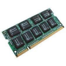
Fig. 4. PageRank on Twitter Graph
TABLE VII
P REPROCESSING T IME (S EC .) OF G RAPH C HI AND VENUS of scanning the structure table is evenly distributed among
processing all vertices, and is not included here. It can be
observed that PSW spends a significant amount of time
Dataset GraphChi VENUS for processing the shards before execution. In contrast, such
Twitter 424 570 waiting time for VSP is much smaller. This is due to that
clueweb12 19,313 18,845 VSP allows to execute the update function while streaming in
Netflix 180 75 the structure data. For example, in the case that the budget of
KDDCup 454 169 main memory is 8GB, PSW spends 749.78 seconds. However,
Synthetic-4M 17 18 VSP-I and VSP-II just needs 104.01 and 102.12 seconds,
Synthetic-6M 23 30 respectively. Note that about the half share of the processing
Synthetic-8M 34 41 time of PSW is spent here, which spends far more time than
Synthetic-10M 47 53 our algorithms.
VSP also generates significantly smaller number of shards
use pagecache-mangagement to disable pagecache in all our 2 than PSW, as shown in Fig. 4(c). For example, in the case
experiments. that the budget of main memory is 0.5GB and 1GB, PSW
generates 90 and 46 number of shards, respectively. And these
The results of processing time are reported in Fig. 4(a), numbers for our algorithms are 15 and 4. This is because VSP
where we can see that VSP is up to 3x faster than PSW spends the main budget of the memory on the value data of a
and ECP. For example, in the case that the budget of main v-shard, while the space needed to keep related structure data
memory is 8GB, PSW spends 1559.21 seconds. ECP also in memory is minimized.
needs 1550.2 seconds. However, VSP-I and VSP-II just need
477.39 and 483.47 seconds, respectively. To further illustrate Fig. 4(d) and Fig. 4(e) show the amount of data write and
the efficiency of VSP, we also examine various performance read, respectively. We observe that the data size written/read
factors including preprocessing, sharding, data access, and to/from disk is much smaller in VSP than in the other systems.
random IOs, as shown below. Specifically, PSW has to write 24.7GB data to disk, and read
the same amount of data from disk, per iteration, regardless
In Fig. 4(b), we compare PSW and VSP in terms of of memory size. These numbers for ECP are 11GB and
the overall waiting time before executing a next shard. For 28GB under 8GB memory budget, which are also very large
PSW, it includes the loading and sorting time of each memory and become a significant setback of ECP in its edge-centric
shard; for VSP, it includes the time to execute unpin calls, streamlined processing. In sharp contrast, VSP only writes
view updates, and merge-join operations. Note that the time 0.24GB, which is 100X and 50X smaller than PSW and ECP,
respectively. In terms of data size of read, VSP reads 12.7-
2 https://code.google.com/p/pagecache-mangagement/ 16.8GB data under various memory budgets. The superiority of
1139Data Size of Write (GB)
Data Size of Read (GB)
5000 1500
PSW PSW 15 PSW 15 PSW
Elapsed Time (sec.)
ECP
Elapsed Time (sec.) ECP ECP ECP
VSP−I VSP−I
4000 VSP−I VSP−I
VSP−II VSP−II VSP−II
VSP−II
1000 10 10
3000
2000
500 5 5
1000
0 0 0 0
Connected Component Community Detection Netflix KDDCup Netflix KDDCup Netflix KDDCup
Task Datasets Task Task
(a) WCC & CD (b) ALS (c) Data Size of Write (d) Data Size of Read
Fig. 5. More Graph Mining Tasks
VSP in data access is mainly due to the separation of structure We compare the total data size being accessed per iteration
data and value data and caching the value data in a fixed buffer. of the four algorithms in Fig. 5(c) and Fig. 5(d). ECP still
accesses more data than we do. For example, ECP has to
Although VSP-I and VSP-II perform very closely, they
access 2.64GB and 8.23GB disk data, including both read
have slight difference in terms of IO performance, as shown
and write, for Netflix and KDDCup, respectively. For VSP-I
in Fig. 4(f). For most cases, VSP-II incurs less IOs than
and VSP-II, these numbers are just 2.41 and 3.96. However,
VSP-I because it is free of maintaining the materialized view
our VSP is slightly slower, because VSP requires more non-
in executing shards. However, when the memory budget is
sequential seeks than ECP. Finally, note that because VSP-I
smaller than 1GB, the number of P increases quickly. In this
and VSP-II are both working in the in-memory mode due to the
case, VSP-II is slower due to the heavy access of the value
small graph size of Netflix and KDDCup, so they read/write
table.
the same amount of data size.
B. Exp-2: More Graph Mining Tasks
After the evaluation under various RAM sizes, we further C. Exp-3: The Synthetic Datasets
compare the four algorithms for other graph mining tasks.
We set the memory budget as 4GB for all algorithms. In To see how a system performs on graphs with increasing
detail, Fig. 5(a) shows the processing time of running WCC data size, we also did experiments over the 4 synthetic datasets.
and CD over Twitter, where our algorithms, VSP-I and VSP- We test with PageRank and WCC, and report the running time
II, clearly outperform the other competitors. For example, in Fig. 6(a) and Fig. 6(b) respectively. Again, we see that VSP
in terms of the WCC task, the existing algorithms, PSW uses just a fraction of the amount of time as compared to the
and ECP, spend 1772.57 and 4321.06 seconds, respectively, other two systems.
while our algorithms spend 942.74 and 972.43, respectively. In general, the processing time increases with the number
In this task, ECP is much slower than PSW. One reason is of vertices. However, the time of PSW and ECP increases
that both PSW and our algorithms can employ the selective much faster than VSP. For example, when the number of
scheduling [3], [19] to skip unnecessary updates on some vertices increases from 4 million to 10 million, the time of
vertices/shards. However, this feature is infeasible for ECP PSW increases by 40.81 and 76.68 seconds for the task
because it is edge-centric and thus cannot support selective of PageRank and WCC, respectively; and the time of ECP
scheduling of vertices. increases by 74.13 and 198.72 seconds. In contrast, the time of
For the CD task, Fig. 5(a) shows the performance of VSP-1 just increases by 21.85 and 49.93 seconds. The superior
PSW and our algorithms. In detail, PSW spends 2317.75 performance of VSP is mainly due to the less amount of data
seconds. VSP-I and VSP-II just need 1614.65 and 1617.04 access per iteration, as shown in Fig. 6(c) and Fig. 6(d).
seconds, respectively. The CD task cannot be accomplished
by ECP, because CD is based on label propagation [17],
where each vertex chooses the most frequent label among its D. Exp-4: On the Web-Scale Graph
neighbors in the update function. The most frequent label can
In this experiment, we compare GraphChi, X-Stream, and
be easily decided in terms of vertex-centric processing, where
VENUS on a very large-scale web graph, clueweb12 [22],
all neighbors and incident edges are passed to the update
which has 978.4 million vertices and 42.5 billion edges. We
function. However, this is not the case for the edge-centric
choose not to use yahoo-web [27] which has been used in
processing while ECP cannot iterate all incident edges and all
many previous works [3], [14], because the density of yahoo-
neighbors to complete the required operation.
web is incredibly low where 53% of nodes are dangling nodes
The next task is ALS, which is tested over both datasets of (nodes with no outgoing edges), and testing algorithms and
Netflix and KDDCup. The overall processing time is given in systems on yahoo-web might give inaccurate speed report. On
Fig. 5(b). In this test, the performance of PSW is much slower the other hand, the number of edges in clueweb12 are an order
than ECP and our algorithms, but ECP is slightly better than of magnitude bigger and only 9.5% of nodes in clueweb12
both VSP-I and VSP-II. For example, in terms of the ALS task are dangling nodes. We run 2 iterations of PageRank for
over KDDCup, PSW spends 1446.01 seconds. ECP spends each system. As shown in Table VIII, VENUS significantly
259.99 seconds. VSP-I and VSP-II spend 357.04 and 190.32 outperforms GraphChi and X-Stream by reading and writing
seconds, respectively. less amount of data.
1140150 350
PSW PSW
ECP ECP
VSP−I 300 VSP−I
Elapsed Time (sec.)
Elapsed Time (sec.)
VSP−II VSP−II
250
100
200
150
50
100
50
0 0
4M 6M 8M 10M 4M 6M 8M 10M
# Vertices # Vertices
(a) PageRank (b) WCC
1.5 6
PSW PSW
ECP ECP
Data Size of Write (GB)
Data Size of Read (GB)
VSP−I 5 VSP−I
VSP−II VSP−II
1 4
3
0.5 2
1
0 0
4M 6M 8M 10M 4M 6M 8M 10M
# Vertices # Vertices
(c) Data Size of Write (d) Data Size of Read
Fig. 6. The Synthetic Datasets
TABLE VIII
E XPERIMENT R ESULTS : PAGE R ANK ON CLUEWEB 12
also work trying to bridge the two categories of systems,
such as GraphX [32]. As a recent branch of graph parallel-
systems, the disk-based graph computing systems, such as
System Time Read Write
GraphChi [3], X-Stream [14], and TurboGraph [15], have
PSW 15,495 s 661GB 661GB shown great potential in graph analytics, which do not need
ECP 26,702 s 1,121GB 571GB to divide and distribute the underlying graph over a number
VSP-I 7,074 s 213GB 43GB of machines, as did in previous graph-parallel systems. And
VSP-II 6,465 s 507GB 19GB remarkably, they can work with just a single PC on very large-
scale problems. It is shown that disk-based graph computing
on a single PC can be highly competitive even compared to
V. R ELATED S YSTEMS
parallel processing over large scale clusters [3].
There are several options to process big graph tasks: it
is possible to create a customized parallel program for each Disk-based systems. The disk-based systems, including
graph algorithm in distributed setting, but this approach is GraphChi [3], TurboGraph [15], and X-Stream [14], are
difficult to generalize and the development overhead can be closely related to our work. Both GraphChi and VENUS
very high. We can also rely on graph libraries with various are vertex-centric. Like our system VENUS, GraphChi also
graph algorithms, but such graph libraries cannot handle web- organizes the graph into a number of shards. However, unlike
scale problems [1]. Recently, graph computing over distributed VENUS which requires only a v-shard to be fit into the mem-
or single multi-core platform has emerged as a new framework ory, GraphChi requires each shard to be fit in main memory. As
for big data analytics, and it draws intensive interests [1], [2], a result, GraphChi usually generates many more shards than
[3], [4], [5], [6], [7], [8], [9], [10], [11]. Broadly speaking, all VENUS under the same memory constraint (Fig. 4(c)), which
existing systems can be categorized into the so-called data- incurs more data transfer (Fig. 4(d) and Fig. 4(e)) and random
parallel systems (e.g. MapReduce/Hadoop and extensions) and IOs. Furthermore, GraphChi starts the computation after the
graph-parallel systems. shard is completely loaded and processes next shard after the
value propagation is completely done. In contrast, VENUS
The data-parallel systems stem from MapReduce. Since enables streamlined processing which performs computation
MapReduce does not support iterative graph algorithms orig- while the data is streaming in. Another key difference of
inally, there are considerable efforts to leverage and improve VENUS from GraphChi lies in its use of a fixed buffer to
the MapReduce paradigm, leading to various distributed graph cache the v-shard, which can greatly reduce random IOs.
processing systems including PEGASUS [5], GBase [9], Gi-
raph [28], and SGC [29]. On the other hand, the graph-parallel The TurboGraph can process graph data without delay, at
systems use new programming abstractions to compactly the cost of limiting its scope on certain embarrassingly parallel
formulate iterative graph algorithms, including Pregel [1], algorithms. In contrast, VENUS can deal with almost every
Hama [7], Kingeograph [10], Trinity [11], GRACE [19], [18], algorithms as GraphChi. Different from VENUS that uses hard
Horton [30], GraphLab [2], and ParallelGDB [31]. There is disk, TurboGraph is built on SSD. X-Stream is edge-centric
1141and allows streamlined processing like VENUS, by storing [7] S. Seo, E. J. Yoon, J. Kim, S. Jin, J.-S. Kim, and S. Maeng, “HAMA:
partial, intermediate results to disk for later access. However, An Efficient Matrix Computation with the MapReduce Framework,” in
CLOUDCOM. Ieee, Nov. 2010, pp. 721–726.
this will double sequential IOs, incur additional computation
cost, and increase data loading overhead. [8] E. Krepska, T. Kielmann, W. Fokkink, and H. Bal, “HipG: Parallel
Processing of Large-Scale Graphs,” SIGOPS Operating Systems Review,
VENUS improves previous systems in several important vol. 45, no. 2, pp. 3–13, 2011.
directions. First, we separate the graph data into the fixed [9] U. Kang, H. Tong, J. Sun, C.-Y. Lin, and C. Faloutsos, “GBASE : A
Scalable and General Graph Management System,” in KDD, 2011, pp.
structure table and the mutable value table file, and use a 1091–1099.
fixed buffer for vertex value access, which almost eliminates
[10] R. Cheng, F. Yang, and E. Chen, “Kineograph : Taking the Pulse of a
the need of batch propagation operation in GraphChi (thus Fast-Changing and Connected World,” in EuroSys, 2012, pp. 85–98.
reducing random IOs). Furthermore, each shard in VENUS is [11] B. Shao, H. Wang, and Y. Li, “Trinity: A distributed graph
not constrained to be fit into memory, but instead, they are engine on a memory cloud,” in SIGMOD, 2013. [Online]. Available:
concatenated together forming a consecutive file for stream- http://research.microsoft.com/jump/183710
lined processing, which not only removes the batch loading [12] J. Dean and S. Ghemawat, “MapReduce: simplified data processing on
overhead but also enjoys a much faster speed compared to large clusters,” in OSDI, vol. 51, no. 1. ACM, 2004, pp. 107–113.
random IOs [14]. Compared to TurboGraph, VENUS can [13] M. Zaharia, M. Chowdhury, M. J. Franklin, S. Shenker, and I. Stoica,
handle a broader set of data mining tasks; compared to X- “Spark : Cluster Computing with Working Sets,” in HotCloud, 2010,
pp. 10–10.
Stream, VENUS processes the graph data just once (instead
[14] A. Roy, I. Mihailovic, and W. Zwaenepoel, “X-Stream: Edge-centric
of twice in X-Stream) and without the burden of writing the Graph Processing using Streaming Partitions,” in SOSP, 2013, pp. 472–
entire graph to disk in the course of computation. 488.
[15] W. Han, S. Lee, K. Park, and J. Lee, “TurboGraph: a fast parallel graph
VI. C ONCLUSION engine handling billion-scale graphs in a single PC,” in KDD, 2013, pp.
77–85. [Online]. Available: http://dl.acm.org/citation.cfm?id=2487581
We have presented VENUS, a disk-based graph compu- [16] C. Engle, A. Lupher, and R. Xin, “Shark: fast data analysis using
tation system that is able to handle billion-scale problems coarse-grained distributed memory,” in SIGMOD Demo, 2012, pp.
efficiently on just a single commodity PC. It includes a novel 1–4. [Online]. Available: http://dl.acm.org/citation.cfm?id=2213934
design for graph storage, a new data caching strategy, and a [17] X. Zhu and Z. Ghahramani, “Learning from labeled and unlabeled
data with label propagation,” Tech. Rep., 2002. [Online]. Available:
new external graph computing model that implements vertex- http://lvk.cs.msu.su/∼bruzz/articles/classification/zhu02learning.pdf
centric streamlined processing. In effect, it can significantly [18] G. Wang, W. Xie, A. Demers, and J. Gehrke, “Asynchronous Large-
reduce data access, minimize random IOs, and effectively Scale Graph Processing Made Easy,” in CIDR, 2013.
exploit main memory. Extensive experiments on 4 large-scale [19] W. Xie, G. Wang, and D. Bindel, “Fast iterative graph computation with
real-world graphs and 4 large-scale synthetic graphs show that block updates,” PVLDB, pp. 2014–2025, 2013. [Online]. Available:
VENUS can be much faster than GraphChi and X-Stream, http://dl.acm.org/citation.cfm?id=2556581
two state-of-the-art disk-based systems. In future work, we [20] A. Aggarwal and J. S. Vlller, “The input/output complexity of sorting
plan to improve our selective scheduling of vertex updates and related problems,” CACM, vol. 31, no. 9, pp. 1116–1127, 1988.
and extend our system to SSD, which will further accelerate [21] H. Kwak, C. Lee, H. Park, and S. Moon, “What is twitter, a social
VENUS greatly. network or a news media?” in WWW, 2010, pp. 591–600.
[22] Evgeniy Gabrilovich, M. Ringgaard, and A. Subramanya, “FACC1:
Freebase annotation of ClueWeb corpora, Version 1 (Release date 2013-
ACKNOWLEDGMENTS 06-26, Format version 1, Correction level 0)”,” http://lemurproject.org/
clueweb12/, 2013.
The work is partly supported by NSFC of China (Grant [23] J. Bennett and S. Lanning, “The netflix prize,” in KDD-Cup Workshop,
No. 61103049) and 973 Fundamental R&D Program (Grant 2007, pp. 3–6. [Online]. Available: http://su-2010-projekt.googlecode.
No.2014CB340304). The authors would like to thank the com/svn-history/r157/trunk/literatura/bennett2007netflix.pdf
anonymous reviewers for their helpful comments. [24] G. Dror, N. Koenigstein, Y. Koren, and M. Weimer, “The Yahoo! Music
Dataset and KDD-Cup’11.” JMLR W&CP, pp. 3–18, 2012.
R EFERENCES [25] R. M. Lawrence Page, Sergey Brin and T. Winograd, “The pagerank
citation ranking: Bringing order to the web,” 1998.
[1] G. Malewicz, M. Austern, and A. Bik, “Pregel: a system for large- [26] Y. Zhou, D. Wilkinson, R. Schreiber, and R. Pan, “Large-scale Parallel
scale graph processing,” in SIGMOD, 2010, pp. 135–145. [Online]. Collaborative Filtering for the Netflix Prize,” in AAIM, 2008, pp. 337–
Available: http://dl.acm.org/citation.cfm?id=1807184 348.
[2] Y. Low, D. Bickson, and J. Gonzalez, “Distributed GraphLab: A [27] “Yahoo! AltaVista Web Page Hyperlink Connectivity Graph, circa
Framework for Machine Learning and Data Mining in the Cloud,” 2002,” http://webscope.sandbox.yahoo.com/.
PVLDB, vol. 5, no. 8, pp. 716–727, 2012. [Online]. Available: [28] “Giraph,” http://giraph.apache.org/.
http://dl.acm.org/citation.cfm?id=2212354
[29] L. Qin, J. X. Yu, L. Chang, H. Cheng, C. Zhang, and X. Lin, “Scalable
[3] A. Kyrola, G. Blelloch, and C. Guestrin, “GraphChi : Large-Scale Graph big graph processing in mapreduce,” in SIGMOD, 2014, pp. 827–838.
Computation on Just a PC Disk-based Graph Computation,” in OSDI,
2012, pp. 31–46. [30] M. Sarwat, S. Elnikety, Y. He, and M. F. Mokbel, “Horton+: A
Distributed System for Processing Declarative Reachability Queries
[4] X. Martinez-Palau and D. Dominguez-Sal, “Analysis of partitioning over Partitioned Graphs,” PVLDB, vol. 6, no. 14, pp. 1918–1929, 2013.
strategies for graph processing in bulk synchronous parallel models,”
in CloudDB, 2013, pp. 19–26. [31] L. Barguñó, D. Dominguez-sal, V. Muntés-mulero, and P. Valduriez,
“ParallelGDB: A Parallel Graph Database based on Cache Specializa-
[5] U. Kang, C. E. Tsourakakis, and C. Faloutsos, “PEGASUS: A Peta- tion,” in IDEAS, 2011, pp. 162–169.
Scale Graph Mining System Implementation and Observations,” in
ICDM. Ieee, Dec. 2009, pp. 229–238. [32] R. Xin, D. Crankshaw, A. Dave, J. Gonzalez, M. Franklin, and I. Stoica,
“GraphX: Unifying Data-Parallel and Graph-Parallel Analytics,” Tech.
[6] R. Chen, X. Weng, B. He, and M. Yang, “Large Graph Processing in Rep., 2014.
the Cloud,” pp. 1123–1126, 2010.
1142You can also read