Determining Solvability in the Birds of a Feather Card Game
←
→
Page content transcription
If your browser does not render page correctly, please read the page content below
The Ninth AAAI Symposium on Educational Advances in Artificial Intelligence (EAAI-19)

                  Determining Solvability in the Birds of a Feather Card Game

        Shuto Araki, Juan Pablo Arenas Uribe, Zach Wilkerson, Steven Bogaerts, Chad Byers
                                                      DePauw University
                                                 Greencastle, IN 46135, U.S.A.
                  {shutoaraki 2020, jarenasuribe 2021, zwilkerson 2020, stevenbogaerts, cbyers}@depauw.edu

                            Abstract                                             A Baseline Approach: Constrained DFS
                                                                             A solvable state has a game tree with at least one leaf repre-
  Birds of a Feather is a single-player card game in which cards
                                                                             senting a single-stack state. Thus one approach for determin-
  are arranged in a grid. The player attempts to combine stacks
  of cards under certain rules, with the goal being to combine               ing solvability is to search for such a leaf. For early-game
  all cards into a single stack. This paper highlights several               states, an exhaustive search is not feasible due to the size
  approaches for efficiently classifying whether a randomly-                 of the tree, but a simple pruning strategy serves as an ef-
  chosen state has a single-stack solution. These approaches                 fective baseline approach (Neller 2018). Specifically, once
  use graph theory and machine learning concepts to prune a                  a solvable child is found, the parent may be declared solv-
  state’s search space, resulting in significant reductions in run-          able, with the other children pruned. Applying this pruning
  time relative to a baseline search.                                        to depth-first search, we call this “Constrained DFS”.

                                                                                                Dataset Generation
                        Introduction                                         This work uses a randomly-generated dataset of 500,000
In this paper we compare several search and machine-                         rows, each consisting of a game state, represented as a string,
learning approaches to determining the solvability of a puz-                 and a binary value indicating whether the state is solvable or
zle game, Birds of a Feather (BoaF) (Neller 2018). In this                   not. The first random choice is the number of stacks, from
single-player game, cards are drawn randomly from a stan-                    1 to 16, followed by the top card for each stack, and finally
dard 52-card deck and placed face up in an r-by-c grid. Here,                the row/column placement of each stack. Constrained DFS
we focus on the r = c = 4 case. Each of the placed cards                     is then used to determine the solvability of the state. Addi-
can be thought of as a stack of size 1. Under certain con-                   tional input features are also generated, to be used by some
ditions, stack x can be moved on top of stack y, forming a                   of the algorithms. Below, two types of input features are de-
single new stack at y’s position with x on top, and leaving                  scribed: graph features and card features.
a blank space at x’s former position. This is allowed only
when x and y are in the same row or column and the stacks’                   Graph Features
top cards meet one of two conditions: 1) they share a suit,                  To consider graph features, we first define two stacks to be
or 2) they have the same or adjacent rank, according to the                  compatible if the top cards are of the same suit, and/or have
ordering A, 2, 3, ..., J, Q, K, where A and K are not adjacent.              the same or adjacent ranks. Note in particular that compat-
The goal of the game is to combine stacks one move at a time                 ibility does not consider the position (row and column) of
using these rules until a single stack remains on the grid. If a             the stack. We then define an undirected graph corresponding
given game state can be reduced to a single stack, then that                 to a state, called a compatibility graph. This graph has one
game state is said to be solvable. Many (but not all) initial                node for each stack, and an edge between nodes indicates
deals are solvable, but moves must be chosen carefully to                    that the corresponding pair of stacks is compatible. Such a
avoid a mistake leading to an unsolvable mid-game state.                     graph is introduced in (Neller 2018).
   This research compares several algorithms for taking a                       Consider a state s with corresponding compatibility graph
game state (starting or mid-game) and determining whether                    g. Suppose s has compatible stacks xs and ys . Therefore, g
or not that state is solvable. Some algorithms achieve 100%                  has an edge between the corresponding nodes xg and yg . If
accuracy through search of a pruned game tree. Others avoid                  xs and ys happen also to be in the same row or column, then
the game tree entirely, aiming for lower execution time, but                 one can be placed on the other. For example, xs might be
also having imperfect accuracy. This paper describes each                    placed on top of ys . In that case, g is updated such that yg
of these algorithms in detail, and concludes with an experi-                 and all edges connected to yg are removed. If, on the other
mental comparison.                                                           hand, xs and ys are not in the same row or column, the edge
                                                                             between xg and yg indicates the potential of the correspond-
Copyright c 2019, Association for the Advancement of Artificial              ing stacks being combined, if future gameplay results in a
Intelligence (www.aaai.org). All rights reserved.                            row or column match.

                                                                      9627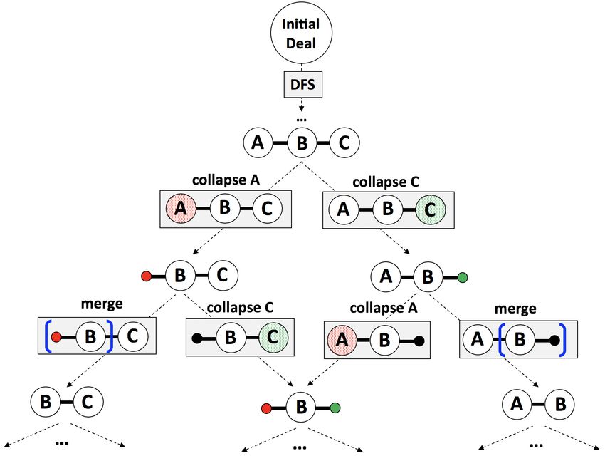
• RC count: For each stack, the number of other stacks in
the same row or column (ignoring compatibility). Across
the state, this can be expressed as a mean RC count, as
well as a median, minimum, and maximum, for example.
• RC compatibility: For each stack, the number of legal
moves available, considering both compatibility and posi-
tion. This can be expressed as minimum, maximum, me-
dian, and mean values across a state.
• Ace count, Kings count: The number of aces and kings in
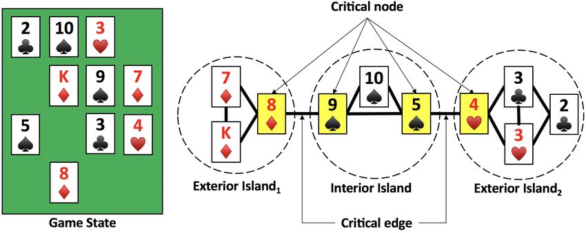
Figure 1: An illustration of compatibility graph definitions the state. These are considered separately from the other
cards, as they have fewer cards with which they are com-
patible by rank.
If a compatibility graph g is disconnected, then the corre- • Rank standard deviation: The standard deviation of ranks
sponding state is unsolvable. To see why, suppose g has two in the state, which corresponds somewhat with the likeli-
subgraphs g1 and g2 that are disconnected from each other. hood that any two stacks are compatible by rank.
That is, there is no path between any node in g1 and any node
in g2 . Gameplay only removes nodes and edges in the com- • Suit ratios: The ratio of the number of cards in a given suit
patibility graph; it never adds them. Therefore, no gameplay to the number of remaining cards in the state, expressed
will create a path between any node in g1 and any node in as single values for each suit.
g2 . Thus, the nodes in these subgraphs are permanently in-
compatible, and so the state is not solvable. Algorithms
On the other hand, a connected compatibility graph is not In this section, four novel solvability classifiers are de-
necessarily solvable, due to row and column requirements scribed: Compatible DFS, Solvability Model, Ordered DFS,
for valid moves. For example, consider a two-stack state and Island Merge. Solvability Model is an approximation al-
with a 9♠ in the upper-right corner, and a 9♣ in the lower- gorithm based on machine learning, while the others achieve
left. The compatibility graph consists of two nodes with an 100% accuracy by searching pruned trees. We describe each
edge between; it is connected. Due to the row/column re- approach here, with comparisons between algorithms in sub-
quirement, however, the state is not solvable. sequent sections.
Figure 1 illustrates several terms for compatibility graphs.
In graph theory, an articulation node is a node in a connected Compatible DFS
graph that, if removed, results in a disconnected graph. Thus, Compatible DFS is simply Constrained DFS (described
a BoaF state can become unsolvable by covering a stack above), with an additional optimization. Using the compati-
corresponding to an articulation node in the compatibility bility graph, Compatible DFS checks if the graph is discon-
graph. We define a critical node as a node in a compatibility nected. If so, then that subtree can be pruned, with the state
graph that is either an articulation node or a node with ex- determined unsolvable. This optimization maintains 100%
actly one connected edge. We also define a critical edge as accuracy, while also reducing the size of the game tree sig-
an edge that connects two critical nodes. nificantly. Below, the performance of this approach is com-
Suppose g1 and g2 are subgraphs of g with no nodes in pared experimentally with several others.
common, and that there is a single edge e connecting these
two subgraphs. Let n1 be the node in g1 connected to e; Solvability Model
similarly for n2 . Therefore, n1 and n2 are critical nodes and The Solvability Model approach uses supervised learning to
e is a critical edge in g. We define g1 and g2 as islands. That create a classifier, with the binary solvability value being the
is, an island is a subgraph that is connected to the rest of target output. We consider several classification algorithms.
the graph via only critical edges. If an island is connected to Mean accuracy results are shown in Table 1. All mod-
the rest of the graph via only one critical edge, it is called els were tested via 10-fold cross-validation, as suggested
an exterior island; otherwise it is an interior island. Again, in (Kohavi 1995), on a set of 500,000 randomly-generated
Figure 1 illustrates these terms. states. For this initial experiment, the default hyperparame-
Finally, we introduce the idea of node connectivity, de- ters of scikit-learn (Pedregosa et al. 2011) and LightGBM
fined as the minimum number of nodes that would have to (Ke et al. 2017) were used for each model. Note that Ta-
be removed to disconnect the compatibility graph. ble 1 also shows results of two baseline models, one always
Given these ideas, the following compatibility graph input returning “solvable,” the other always “unsolvable.” Every
features are computed: minimum, maximum, median, and other model’s accuracy surpasses these baselines. The most
mean degree; critical node, critical edge, and island counts; accurate model is LightGBM, achieving 94.44% accuracy.
is connected or not; and node connectivity. LightGBM is an open-source machine learning algorithm
implementation, with both classification and regression ver-
Card Features sions available. While a full discussion is beyond the scope
Several useful features of a given state can be generated via of this paper, we provide a few key points. LightGBM uses
simple counts and descriptive statistics: gradient tree boosting, in which an ensemble of regression
9628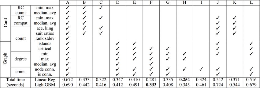
Model                          Accuracy                           The challenge in Ordered DFS is to balance the time of
 LightGBM (Ke et al. 2017)                   0.94443                        execution of the regression model with the benefit of more
 Bagging                                     0.94393                        precise estimates for sibling ordering. Two ideas can be con-
 Multilayer Perceptron                       0.94026                        sidered to strike this balance. First, if the full set of features
 AdaBoost                                    0.93616                        described above is too expensive, then perhaps some subset
 Random Forest                               0.93579                        of features can provide a more effective balance. Second,
 Gradient Boosting Classifier                0.93300                        ordering may be applied selectively. Such ideas may bring
 Stochastic Gradient Descent                 0.92962                        increased processing speed per node, but may also lead to in-
 Logistic Regression                         0.92741                        creased ordering error, meaning less pruning. Thus a careful
 Decision Tree                               0.91853                        balance of tradeoffs is considered in the experiments below.
 Always Unsolvable                           0.51225
                                                                            Input Feature Cost-Performance Analysis This first ex-
 Always Solvable                             0.48775                        periment considers the tradeoff that a greater number and
                                                                            complexity of input features leads to an improved order, but
  Table 1: Accuracy in the testing set for various models.                  also longer ordering time. We refer to a particular experi-
                                                                            mental configuration as an Ordered DFS system. In this ex-
                                                                            periment, each system varies in the subset of features used,
trees are built, with each tree hopefully correcting some er-               and is based on either LightGBM or linear regression. Light-
ror of the previous trees. One insight of LightGBM is in the                GBM is considered because it is the most accurate in the
order of tree construction. A best-first, rather than breadth-              Solvability Model work above. Linear regression is consid-
first, approach is used, in which the leaf with the highest                 ered for its great simplicity and speed, as a counterbalance
prediction error is chosen for expansion first (Shi 2007). In               to the comparative complexity of LightGBM.
addition, LightGBM uses histograms to discretize each con-                     Rather than explore every possible feature subset, subsets
tinuous feature (Ranka and Singh 1998). The discrete bins                   are chosen based on 1) relationships between feature calcu-
of a histogram dictate the subsets into which the data is split             lation requirements, and 2) time of calculation. For example,
on that feature in tree construction, and what branch is fol-               once the expense of looping through a state is undertaken to,
lowed in application of the model. The use of histograms for                say, count the number of aces, the program might as well
discretization also allows smaller data types to be used, thus              count the number of kings, as well as the suits (for suit ra-
reducing memory usage (Li, Wu, and Burges 2008).                            tios) and open spaces (for RC count values), among other
   As LightGBM achieves the highest score of all of the                     card features. Similarly each graph feature requires the com-
tested models, it is chosen for hyperparameter tuning via a                 patibility graph. If any one graph feature is included, then
grid search. A grid search is an algorithm tuning process in                the remaining ones can be included at little additional cost.
which many models are created and tested. Each model is                     Exceptions to this grouping approach occur in some more
defined with a different combination of multiple hyperpa-                   expensive calculations, like island count. Finally, note that
rameter values in an effort to find the ideal hyperparameters.              the number of stacks is not considered in any feature subset
Using 10-fold cross-validation to tune learning rate, num-                  for Ordered DFS, since Ordered DFS always compares sib-
ber of estimators, and number of leaves simultaneously, the                 lings, and siblings always have the same number of stacks.
ideal combination is 0.2, 50, and 90, respectively. This tuned                 Twelve subsets of features are tested here, as listed in Ta-
LightGBM model increases the mean accuracy to 94.479%,                      ble 2. This leads to 24 Ordered DFS systems using either
and thus is used as the canonical Solvability Model in algo-                linear regression or LightGBM. In either case, the default
rithm comparison experiments below.                                         scikit-learn hyperparameters are used. The model is trained
   Unfortunately, at 94.479% accuracy, the tuned LightGBM                   on a 500,000-element random dataset, using only the des-
model is still not accurate enough to be used reliably in                   ignated subset of features. The resulting model is used in
solvability prediction. Furthermore, due to the complexity of               Ordered DFS. Each such Ordered DFS system is tested on a
some of the input features, this model is also fairly slow; in              separate randomly-generated 100,000-element test set.
fact, for a state with less than six cards, it is typically faster             The last two rows of Table 2 show that input feature sub-
to use a search algorithm. We revisit the use of a machine                  sets F and H lead to the fastest average search times for
learning model in our discussion of Ordered DFS.                            LightGBM and linear regression, respectively. Subset F uses
                                                                            all graph features except the most expensive, island count.
Ordered DFS                                                                 Its effectiveness demonstrates the value of the compatibility
                                                                            graph, despite its cost. Subset H also performs well in linear
Returning now to search algorithms with 100% accuracy,                      regression, perhaps suggesting that the three features in sub-
note that both Constrained DFS and Compatible DFS search                    set H are most important of all, and that the others in subset
siblings in arbitrary order. If a solvable child is found, the              F require a more sophisticated model to maximize utility.
remaining unvisited siblings are pruned. So more pruning
occurs if a solvable child is found sooner. Thus, Ordered                   Algorithm Behavior in Ordered DFS Given the results
DFS places siblings in a priority queue, with higher priority               of the previous experiment, we explore further LightGBM
assigned to children with a greater estimated likelihood of                 with feature subset F and linear regression with feature sub-
solvability. This is estimated using a regression model simi-               set H. Additional data are provided in Table 3. Before con-
lar to the Solvability Model classifiers described above.                   sidering these results, several facts must be established.

                                                                     9629
Table 2: 12 subsets of features and average total search time for each subset
Lin. Reg., H LightGBM, F overhead beyond just prediction time that is not captured in
Pred. Time (×10−5 s) 0.016 0.578 Table 3. More importantly, though, note that predictions are
RMSE 0.400 0.256 made for far more nodes than are actually counted in the
Node Count 1381 1045 “node count” measure. Predictions must be made for every
Total Time (s) 0.254 0.333 generated child to create an ordering. If the ordering is ef-
fective and a solvable child is found quickly, then most of
Table 3: Additional performance data for linear regression those children will be pruned (thus not “counted”), while a
(subset H) and LightGBM (subset F). prediction was nevertheless determined for each.
Having established the meanings of these measures, con-
sider the results in Table 3. LightGBM has a lower average
RMSE than linear regression, at 0.256. This is not surpris-
The prediction time and RMSE rows of Table 3 cor-
ing, given the increased sophistication of LightGBM over
respond to results about the estimation models them-
linear regression. Lower error means more effective order-
selves, separate from Ordered DFS. Each model was tested
ing, and thus more pruning. This is reflected in the fact that
via 10-fold cross validation on the same 500,000-element
LightGBM also has a lower average node count than linear
randomly-generated dataset. Prediction time refers to the av-
regression, at 1045. However, it also is not surprising that
erage time to estimate solvability per state. RMSE refers to
this low error requires a higher prediction time per node, at
the average root-mean-squared error in estimating solvabil-
0.578 × 10⁻⁵ s.
ity, where the estimated value is compared to a target value
of 1 for solvable states and 0 for unsolvable states. Thus, Linear regression has a worse RMSE and therefore a
for RMSE a lower number is better. Note that a prediction higher node count than LightGBM. Its prediction time, on
of “unsolvable” for every state results in an RMSE of 0.698 the other hand, is much faster. This faster prediction time
for this dataset. Also note that this RMSE measure for re- results in a faster total time, despite the higher node count.
gressors is distinct from the accuracy measure for classifiers Since linear regression on feature subset H is slightly faster
used in the Solvability Model discussion above. than LightGBM on subset F, we consider further the linear
regression model in Ordered DFS in the next experiment.
The node count and total time rows of Table 3 corre-
spond to results about the application of each of the esti- Ordering Cutoff Tuning Despite the results above, even a
mation models to Ordered DFS. After training each estima- linear regression model on subset H applied to Ordered DFS
tion model on the same 500,000-element random dataset, is slower than Compatible DFS, with average total times
the resulting Ordered DFS system conducts a search on each of 0.252s and 0.140s, respectively. In an effort to improve
element in a separate randomly-generated 100,000-element Ordered DFS’s results, this next experiment considers the
test set. The node count corresponds to the average number selective application of ordering. Note that ordering of sib-
of nodes that are “processed” – that is, the number of nodes lings is less useful in late-game states than early-game states.
checked for being terminal or having a disconnected com- Late-game states have trees with fewer levels, and so the
patibility graph, followed by node expansion if warranted. benefits of pruning siblings decreases, while the solvability
A lower node count means more effective pruning has oc- estimation cost per child remains the same. A new order-
cured. The total time column is the average total amount of ing cutoff hyperparameter allows more selective application
time that an Ordered DFS search requires. of sibling ordering, by specifying the number of stacks in
It is also important to note that prediction time × node a state for which such ordering will no longer be done. For
count 6= total time, for two reasons. First, there is additional example, with an ordering cutoff value of 5, Ordered DFS
9630Island Merge
Another algorithm that uses graph features for pruning is Is-
land Merge. Recall the definitions of exterior and interior
island, critical node, and critical edge, as illustrated in Fig-
ure 1. Islands are important because with the exception of
critical nodes, to maintain solvability requires that stacks in
an island be moved to cover only other stacks in the same
island. Critical nodes and edges must be handled correctly
to avoid a disconnected compatibility graph and therefore
unsolvable state.
Island Merge is a search based on Compatible DFS, but
with further pruning based on compatibility graph analy-
sis. As gameplay progresses, more stacks are covered, and
thus more nodes are removed from the compatibility graph.
This means fewer edges in the compatibility graph and a
greater chance of critical nodes and edges. Island Merge
tracks these graph features. While we do not provide here a
Figure 2: Effect of ordering cutoff on Ordered DFS average formal proof of correctness, the algorithm described below
total time achieves 100% accuracy on a test set of 500,000 randomly-
generated states.
The key idea of Island Merge is that each island can be
performs sibling ordering only for states with greater than treated as a “mini-game” of BoaF. To collapse an island is
five stacks. Otherwise, an arbitrary ordering is used, and no to make a series of moves reducing that island to a single
solvability estimation cost is incurred – just as in Compati- stack, essentially solving that mini-game. In the same way
ble DFS. that a full BoaF game state may be unsolvable even with
a connected compatibility graph, an island may also be un-
The lowest sensible ordering cutoff value is 2, meaning collapsible even with a connected compatibility (sub)graph.
that all children will be ordered except for children of two- Thus, an attempted collapse operation may fail.
stack states. It never makes sense to order the children of Exterior islands should be collapsed before interior is-
a two-stack state, as would be done with ordering cutoff lands. This is because an interior island typically has at least
1. This is because all two-stack states have either zero or two critical nodes; the process of collapsing will inherently
two children. Zero children means the two-stack state is an cover one of them, thereby severing the connection to the
unsolvable state, and of course there are no children to or- corresponding island. Thus, Island Merge prunes the tree
der. Two children means the two-stack state is solvable by such that only exterior island-collapsing moves are consid-
putting either stack on the other, with the only difference be- ered. In rare circumstances, an interior island could be col-
ing which stack ends up on top. Thus, ordering of these two lapsed first if it has just one critical node with multiple criti-
states is irrelevant. cal edges, but exterior islands may always be collapsed first.
In this experiment, then, 15 Ordered DFS systems are In addition to collapsing, Island Merge uses a second op-
considered, with ordering cutoffs from 2 to 16. Other char- eration, merging. Suppose s is a single-stack exterior island
acteristics of the systems use the conclusions from previous adjacent to another island a. To merge s into a is to consider
experiments. Each uses linear regression, since that was the s as part of a when collapsing a. If a is an interior island con-
best model in the previous experiment. Each also uses fea- nected to a set of islands E, then a becomes an exterior is-
ture subset H – the best subset found for linear regression in land when all but one island in E is merged with a. In short,
the first Ordered DFS experiment. under the stated conditions, merging converts an island from
interior to exterior, making it eligible for collapsing.
Results are in Figure 2. The curve shows the average At a high level, then, Island Merge chooses between these
search time for Ordered DFS with linear regression for each two operations: to collapse an exterior island, or to merge
ordering cutoff. For comparison, the straight line shows the a single-stack exterior island with another island. If a col-
performance of Compatible DFS, which does not consider lapse operation is chosen, then moves not corresponding to
ordering cutoff at all. Note, as expected, that Ordered DFS collapsing that island can be pruned, until the collapse is
with ordering cutoff 16 is equivalent to Compatible DFS, complete or it fails. If a merge operation is chosen, then the
plus a bit of overhead. With ordering cutoffs below 9, the single-stack exterior island is considered part of another is-
tree is small enough that the effort spent ordering does not land, and then a new high-level operation is chosen.
lead to significant enough pruning to be worthwhile. The This exploration of high-level operations can be mod-
ideal ordering cutoff is 11. eled as a search in an island tree, as illustrated in Figure 3.
Based on this series of experiments, the ideal Ordered Initially, the game tree is explored via ordinary Compati-
DFS system uses linear regression with feature subset H and ble DFS, as shown with the “DFS” marker at the top of
ordering cutoff 11. This system is used in the comparison the tree. This continues with each new state generated by
experiments described below. a player move, until the current game state comes to have
9631Figure 3: Game tree for island merge
multiple islands. At this time, Island Merge chooses from Figure 4: Comparison of the average runtime for each algo-
available high-level operations. For example, in Figure 3, rithm.
we show three islands near the root of the tree, indicated
by A − B − C . Note that B is an interior island, while A
and C are exterior islands, and so the algorithm can choose ten stacks.
to collapse either A or C. Suppose the algorithm chooses to Consider Figure 4. Solvability Model (with LightGBM)
attempt to collapse A. In that case, a successful collapse (if has the fastest running time in the divergent region, at
it exists) is found and the algorithm moves on to the next 1.9822×10⁻⁶ seconds. Note, however, that Solvability
high-level decision. At that point, it either merges A into Model has imperfect accuracy, at 94.479%. Among the
B or collapses C. If required due to exclusively unsolvable 100% accuracy algorithms, Ordered DFS consistently has
states further down the tree, the algorithm backtracks to find the fastest runtime in the divergent region. Compatible DFS
an alternative successful collapse of A (if it exists). If no has the second-fastest runtime, followed by Island Merge. In
successful collapses of A exist, or none lead to ultimately the convergent region, however, the time needed to search
solving the game, then backtracking occurs one level higher the game tree is less than that required to apply Solvabil-
in the island tree, such that the algorithm attempts to collapse ity Model’s prediction strategy. Thus, the Solvability Model
C instead of A. This process continues until either a solved is the slowest algorithm in that region, but only by a very
state is found and the search returns “solvable”, or all moves small margin. Furthermore, since Constrained DFS has the
result in unsolvable states, and the search returns “unsolv- fastest per-node runtime, it has the fastest overall runtime in
able”. Below, the performance of Island Merge is compared the convergent region; again, though, the difference is very
with the other algorithms of this paper. small.
Figure 5 highlights the fact that Island Merge searches the
Algorithm Comparison fewest nodes in the divergent region. Ordered DFS comes in
Each algorithm is evaluated based on runtime and nodes a close second, followed by Compatible DFS. The Solvabil-
searched, using a dataset of 248,170 randomly-generated ity Model cannot be considered in this comparison, since it
states. All tests are conducted using a local parallel com- does not explore the game tree. Even though Island Merge
puting network of 20 computers running Ubuntu 16.04 with has the highest per-node runtime, its reduced number of
a 4-core Intel i5-2400 CPU and 8GB of RAM each. nodes explored suggests that it may have the fastest poten-
Figures 4 and 5 illustrate the mean performance of tial runtime of all experimental algorithms. Additionally, all
each algorithm in terms of runtime and number of nodes three experimental algorithms search nine to ten times fewer
searched, respectively. These data suggest that the number nodes than Constrained DFS on average.
of nodes explored is the greatest influence on runtime. They In Figure 5, it is interesting to note the small rise in nodes
also demonstrate improvements by all experimental algo- examined for Constrained DFS for lower numbers of stacks.
rithms, both in runtime and nodes searched, relative to Con- This is because the fewer stacks a randomly-generated state
strained DFS. This advantage tapers off as the number of has, the less likely that it is solvable. Since Constrained DFS
stacks in the state decreases, to the point where differences prunes only when a solvable node is found, unsolvable states
in performance between algorithms are comparatively small. will result in no pruning, and thus a higher count of nodes
Thus, the data can be separated into two major regions: the examined. This does not occur in the other algorithms, how-
divergent region concerning states with at least ten stacks, ever, because their pruning is based on not only solvability,
and the convergent region concerning states with less than but also the compatibility graph.
9632dent in multi-player games such as checkers (Samuel 1959),
chess (Campbell, Hoane Jr., and Hsu 2002), and Go (Sil-
ver et al. 2016), since the strategy of the solver is depen-
dent upon an unknown sequence of opposing moves. How-
ever, planning is still necessary in relaxed, single-player ver-
sions of these games, as well as games such as FreeCell
(Paul and Helmert 2016; Elyasaf, Hauptman, and Sipper
2011) and solitaire (Bjarnason, Tadepalli, and Fern 2007;
Helmstetter and Cazenave 2003), where optimal play may
be defined by various independent factors. BoaF may also be
included in this group, as many similarly independent prop-
erties of stacks exist. These properties influence branching
in the game tree and in the path to a solution.
However, BoaF differs significantly in that the number of
moves for each solution is identical. That is, while cycling
through the deck in solitaire and using free cells in Free-
Cell lead to solutions of varying length, every solution to a
solvable BoaF state with n stacks is n − 1 moves long. As
a result, there is less emphasis in BoaF on efficient moves
as there is on accurate moves, and algorithms accordingly
Figure 5: Comparison of the average number of nodes ex-
focus more on intelligent move selection and pruning of the
plored for each algorithm.
search space. This logic relates to work on deadlock patterns
by Paul and Helmert (2016), and is strikingly similar to ideas
proposed by Helmstetter and Cazenave (2003). In fact, many
Considering both figures, there is a comparatively large
parallels exist in limitations and patterns based on state po-
difference between the three experimental algorithms and
sitions in BoaF and Gaps (Helmstetter and Cazenave 2003).
Constrained DFS – but is this difference significant? Since
the data used to generate Figures 4 and 5 is not normal, we
cannot use standard deviation to determine statistical signif-
icance. However we use a T-test to show that each algorithm Conclusions and Future Work
is significantly different from the others, since the sample
size is statistically large. Specifically, the largest p-value This research presents several BoaF solvability classifier al-
among all pairwise combinations of algorithms in the fig- gorithms. The most effective algorithm tested is Ordered
ures is less than 0.0001, suggesting statistical significance. DFS with linear regression, feature subset H (a few key
Interestingly, while Compatible DFS is not the fastest al- graph features), and ordering cutoff 11. Other tested strate-
gorithm, its overall performance is comparable to Ordered gies are nearly as effective, and all show significant improve-
DFS and Island Merge. The reasonably strong performance ment over the baseline Constrained DFS approach in run-
of Compatible DFS, which checks only for compatibility time and search space size.
graph connectivity, suggests that this feature is critical in de- These advancements also open various avenues for fur-
veloping an efficient search-based classifier. ther research. Potential further optimizations exist for many
algorithms, such as repeated island detection in Island
Related Work Merge. Additionally, features that would require an exhaus-
Games frequently serve as the context for developing op- tive search to generate may be estimated via efficient ex-
timization algorithms, since many are NP-complete despite ploration of the search space. For example, score is calcu-
having a simple rule set. That is, their large search space lated as the square of the number of cards in each stack in
makes an exhaustive search of potential moves intractable. a terminal or unsolvable state. Thus, mean score for a state
This prompts the development of heuristics and pruning may be estimated via an Island Merge-based approach, as is-
strategies to maximize efficiency with minimal losses to ac- land size could predict maximum stack sizes for unsolvable
curacy. BoaF is an example of a game with perfect informa- states. Score metrics could inform evaluation of state diffi-
tion, since no relevant game information is hidden from the culty, and/or evolutionary generation of difficult states. Test-
player. Since BoaF is newly-developed, no research exists ing states with different row/column dimensions could en-
particularly for this game, but much related work exists for courage novel algorithm strategies, owing to different search
other perfect information games. space sizes, compatibility graph connectivity, and/or posi-
Solver algorithms are designed to maximize play accu- tional limitations. Lastly, a greedy solver algorithm is a natu-
racy for a multi-dimensional problem, since a successful ral extension of the proposed search algorithms, as they find
game is often determined by more than one characteristic. the solution of any state declared solvable. Focusing on a
This idea of a nonlinear solution-finding process highlights solver could employ score-based decisions, as well as el-
the need for planning on the part of the solver (Hoffman ements of Monte-Carlo tree search, to build on intelligent
and Nebel 2001). Multidimensional planning is most evi- ordering and pruning methods outlined in this paper.
9633References 2016. Mastering the game of Go with deep neural networks
Bjarnason, R.; Tadepalli, P.; and Fern, A. 2007. Searching and tree search. 529:484–489.
solitaire in real time. ICGA 131–142.
Campbell, M.; Hoane Jr., A. J.; and Hsu, F.-h. 2002. Deep
blue. Artificial Intelligence 134(2):57–83.
Elyasaf, A.; Hauptman, A.; and Sipper, M. 2011. GA-
FreeCell: evolving solvers for the game of FreeCell. In 13th
Annual Genetic and Evolutionary Computation Conference,
GECCO ’11, 1931–1938.
Helmstetter, B., and Cazenave, T. 2003. Searching with
analysis of dependencies in a solitaire card game.
Hoffman, J., and Nebel, B. 2001. The FF planning system:
Fast plan generation through heuristic search. Journal of
Artificial Intelligence Research 14:253–302.
Ke, G.; Meng, Q.; Finley, T.; Wang, T.; Chen, W.; Ma, W.;
Ye, Q.; and Liu, T.-Y. 2017. Lightgbm: A highly effi-
cient gradient boosting decision tree. In Guyon, I.; Luxburg,
U. V.; Bengio, S.; Wallach, H.; Fergus, R.; Vishwanathan,
S.; and Garnett, R., eds., Advances in Neural Information
Processing Systems 30. Curran Associates, Inc. 3146–3154.
Kohavi, R. 1995. A study of cross-validation and bootstrap
for accuracy estimation and model selection. In Proceed-
ings of the 14th International Joint Conference on Artificial
Intelligence - Volume 2, IJCAI’95, 1137–1143. San Fran-
cisco, CA, USA: Morgan Kaufmann Publishers Inc.
Li, P.; Wu, Q.; and Burges, C. J. 2008. Mcrank: Learning
to rank using multiple classification and gradient boosting.
In Advances in neural information processing systems, 897–
904.
Neller, T. 2018. “birds of a feather” solitaire card game.
http://cs.gettysburg.edu/ tneller/puzzles/boaf/. Accessed:
2018-07-11.
Paul, G., and Helmert, M. 2016. Optimal solitaire game
solutions using A* search and deadlock analysis. In Pro-
ceedings of the Ninth International Symposium on Combi-
natorial Search, SoCS 2016, 135–136.
Pedregosa, F.; Varoquaux, G.; Gramfort, A.; Michel, V.;
Thirion, B.; Grisel, O.; Blondel, M.; Prettenhofer, P.; Weiss,
R.; Dubourg, V.; Vanderplas, J.; Passos, A.; Cournapeau, D.;
Brucher, M.; Perrot, M.; and Duchesnay, E. 2011. Scikit-
learn: Machine learning in Python. Journal of Machine
Learning Research 12:2825–2830.
Ranka, S., and Singh, V. 1998. Clouds: A decision tree clas-
sifier for large datasets. In Proceedings of the 4th Knowledge
Discovery and Data Mining Conference, 2–8.
Samuel, A. L. 1959. Some studies in machine learning using
the game of checkers. IBM Journal of research and devel-
opment 3(3):210–229.
Shi, H. 2007. Best-first decision tree learning. Ph.D. Dis-
sertation, The University of Waikato.
Silver, D.; Huang, A.; Maddison, C.; Guez, A.; Sifre, L.;
van den Driessche, G.; Schrittwieser, J.; Antonoglou, I.;
Panneershelvam, V.; Lanctot, M.; Dieleman, S.; Grewe, D.;
Nham, J.; Kalchbrenner, N.; Sutskever, I.; Lillicrap, T.;
Leach, M.; Kavukcuoglu, K.; Graepel, T.; and Hassabis, D.
9634You can also read