Brazilian climate normals for 1981-2010 - Scielo.br
←
→
Page content transcription
If your browser does not render page correctly, please read the page content below
Brazilian climate normals for 1981–2010
         Francisco de Assis Diniz(1), Andrea Malheiros Ramos(1) and Expedito Ronald Gomes Rebello(1)
(1)
    Instituto Nacional de Meteorologia, Eixo Monumental Sul, Via S1, Sudoeste, CEP 70680-900 Brasília, DF, Brazil. E-mail:
diretor.inmet@inmet.gov.br, andrea.ramos@inmet.gov.br, expedito.rebello@inmet.gov.br

      Abstract – In the last decades, especially since 2000, the natural vulnerability of Earth’s climate system has
      been a cause of great concern as to the status of global climate change due to the interference of natural and/
      or anthropic activities. Instituto Nacional de Meteorologia (Inmet), the government body officially responsible
      for monitoring weather and climate in Brazil, and also a member of the World Meteorological Organization
      (WMO), is proud to release the new edition of the climate normals for the period of 1981–2010. The new
      edition aims to analyze and register the climate changes that occurred during the two decades following
      the previous edition of 1961–1990. For that purpose, Inmet created a working group to prepare and edit
      these normals, as a basis of knowledge for different spheres of meteorology, aiming to strengthen the study
      and research of climate variability, as well as the Paris Agreement, which limits global warming to 1.5°C
      above pre-industrial levels. Finally, the publication intends to offer guidance, information, and assistance
      to the communities of climate sciences, agribusiness, and public and private institutions, both national and
      international. Overall, activities related to climate have expanded in practically every sphere of human life,
      especially in the fields of science and public policies.
      Index terms: climate, environment, meteorological variables, society.

                             Normais climatológicas do Brasil 1981–2010
      Resumo – Nas últimas décadas, principalmente desde 2000, a vulnerabilidade natural do sistema climático
      da Terra tem causado preocupações quanto à mudança climática global devido a processos naturais e/ou
      atividades antropogênicas. O Instituto Nacional de Meteorologia (Inmet), responsável por monitorar o tempo
      e o clima no Brasil, e também membro da Organização Meteorológica Mundial (OMM), tem o orgulho de
      lançar a nova edição das normais climatológicas 1981–2010. Esta nova edição visa analisar e registrar as
      mudanças climáticas que ocorreram durante as duas décadas após a edição anterior de 1961–1990. Com
      esse propósito, o Inmet criou um grupo de trabalho para preparar e editar essas normais, como base para
      conhecimento em diferentes esferas da meteorologia, para fortalecer o estudo e a pesquisa da variabilidade
      climática, bem como o Acordo de Paris, que limita o aquecimento global a 1,5°C acima dos níveis da era pré-
      industrial. Por fim, a publicação visa oferecer diretrizes, informações e assistência a comunidades de ciências
      climáticas, agronegócios, instituições públicas e privadas, tanto no âmbito nacional quanto internacional. No
      geral, as atividades relacionadas ao clima têm expandido em praticamente todas as esferas da vida humana,
      sobretudo nas áreas de ciências e políticas públicas.
      Termos para indexação: clima, meio-ambiente, variáveis meteorológicas, sociedade.

                      Introduction                                  stations for which the most recent climate normal is
                                                                    unavailable, whether because the station was not in
   According to the technical regulations of World                  operation for a period of 30 years or any other reason,
Meteorological Organization (WMO, 1989), “normals”                  “provisional normals” can be calculated; these are
are defined as the averages computed over a uniform                 short-term averages, based on observations extending
and relatively long period, which should cover at                   over a minimum period of 10 years.
least three consecutive 10-year periods. The same                      In 1989, aiming to establish general procedures
regulations define “climatological standard normals”                for the calculation of monthly and annual averages
as the averages of climatological data calculated for               for the period of 1961–1990 and subsequent years,
the following consecutive 30-year periods: January                  WMO published the Technical Document WMO-TD/
1, 1901, to December 31, 1930, and January 1, 1931,                 No. 341 (WMO, 1989), which allows determining
to December, 31, 1960, and so forth. In case there are              climatological standard normals and provisional

           This is an open-access article distributed under the         Pesq. agropec. bras., Brasília, v.53, n.2, p.131-143, Feb. 2018
           Creative Commons Attribution 4.0 International License                         DOI: 10.1590/S0100-204X2018000200001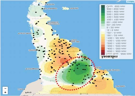
132                                                         F. de A. Diniz et al.

normals, further suggesting other climate variables.                     accumulated precipitation; absolute maximum value
Coherently, it was established that all member countries                 for accumulated precipitation in 24 hours; number
should comply with these procedures. According                           of days within a month or a year with precipitation
to WMO, climate data are often more useful when                          greater or equal to 1 mm; 10-day precipitation; number
comparable with climatological standard normals,                         of days within a period of 10 days with precipitation
which should be obtained according to their own                          greater or equal to 1 mm; number of periods with 3 or
technical recommendations. Therefore, the calculation                    more consecutive days without precipitation; number
and publication of climatological “standard” normals                     of periods with 5 or more days without precipitation;
is of utmost importance. In the absence of these, due                    and number of periods with 10 or more consecutive
to the nonexistence or poor quality of data, the use                     days without precipitation.
of “simple” or “provisional” normals are acceptable                         This paper aims to present the updated version of
alternatives.                                                            the Brazilian climate normals for the period of 1981–
   In Brazil, as systematic meteorological observations                  2010 (Inmet, 2018). This new publication was initially
only began in 1910, the meteorological service of                        motivated by the interest to widely disseminate the
Ministério da Agricultura, Pecuária e Abastecimento                      normals for the period established by WMO, updating
published the first climate normals in 1970, referring to                the meteorological variables of 1961–1990 to 1981–
the period of 1931–1960 (Brasil, 1970). The publication                  2010, in addition to aggregating new meteorological
was restricted to monthly and annual average values                      parameters as requested by the general community
of the following variables: atmospheric pressure,                        that uses the normals for several types of studies. Even
maximum temperature, minimum temperature,                                though agroclimatology stands as the main technical
absolute maximum temperature, absolute minimum
                                                                         area benefiting from the information provided in this
temperature, mean temperature, relative humidity,
                                                                         publication, virtually all human activity depends on
cloudiness, total precipitation, maximum precipitation
                                                                         climatological information, from the productive to
in 24 hours, total evaporation, and total insolation.
                                                                         the public health sector, and from sport activities to
   In 1992, Instituto Nacional de Meteorologia (Inmet),
                                                                         leisure, for example.
then called Departamento Nacional de Meteorologia
                                                                            The normals presented here in the form of tables
of Ministério da Agricultura e Reforma Agrária,
                                                                         and maps correspond to the following variables:
published the 1961–1990 climate normals (Brasil,
                                                                          1. compensated average temperature (°C);
1992), gathering data from 209 weather stations,
comprising the same set of variables as the 1931–1960                     2. maximum temperature (°C);
normals.                                                                  3. minimum temperature (°C);
   In 2009, commemorating the centennial of the                           4. dew-point temperature (°C);
institution, an updated and expanded version of the                       5. wet-bulb average temperature (°C);
Brazilian climate normals for the period of 1961–1990                     6. absolute value of maximum temperature (°C);
(Ramos et al., 2009) was published. Data from 411                         7. absolute value of minimum temperature (°C);
surface weather stations of Inmet, all operational in                     8. absolute value of minimum wet-bulb temperature (°C);
that period, were analyzed according to the procedures                    9. number of days with maximum monthly and annual
recommended by WMO. The studied variables,                               temperatures for ≥ 25°C;
presented in the form of tables and maps, were                            10. number of days with maximum monthly and
expanded to 31: compensated average, maximum, and                        annual temperatures for ≥ 30°C;
minimum temperatures; absolute maximum values of                          11. number of days with maximum monthly and
maximum and minimum temperatures; atmospheric                            annual temperatures for ≥ 35°C;
pressure (hPa) at a station level; insolation; evaporation;               12. number of days with maximum monthly and
wind intensity, prevailing and resulting direction, and                  annual temperatures for ≥ 40°C;
zonal and meridional components; monthly and hourly                       13. number of days with minimum monthly and
cloudiness at 00:00, 12:00, and 18:00 Coordinated                        annual temperatures for ≥ 10°C;
Universal Time (UTC); monthly and hourly air                              14. atmospheric pressure (hPa) at a barometer level;
relative humidity at 00:00, 12:00, and 18:00 UTC;                         15. pressure (hPa) at mean sea level;

Pesq. agropec. bras., Brasília, v.53, n.2, p.131-143, Feb. 2018
DOI: 10.1590/S0100-204X2018000200001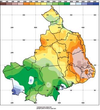
Brazilian climate normals for 1981–2010                                              133

 16. average vapor pressure (mB) calculated by the             risks (whether low, medium, or high) of implementing
Tetens equation;                                               a determined crop in a particular region, in order
 17. total insolation (hours);                                 to ensure water and food security, considering that
 18. total evaporation (mm) using the Piché                    each crop depends on several parameters, such as the
evaporimeter;                                                  amount of water available. In recent years, extreme
 19. cloudiness (tenths);                                      climate events have become more frequent, directly
 20. hourly cloudiness (tenths);                               impacting societies due to associated natural disasters,
 21. compensated air relative humidity (%);                    which are attributed to climate type, topographical
 22. hourly average air relative humidity (%);                 layout, and the established urban occupation (Pachauri
 23. absolute maximum value of relative humidity (%);          & Meyer, 2014).
 24. absolute minimum value of relative humidity (%);             Many of these events have been reported in studies
 25. accumulated precipitation (mm);                           on anomalies in meteorological variables such as
 26. absolute maximum value of accumulated 24-hour             precipitation, temperature, atmospheric pressure,
precipitation monthly and anual (mm);                          wind, air humidity, and the analyses of their respective
 27. number of days, within a period of 10 days, with          deviations. The normal state of these variables shows
precipitation greater or equal to 1 mm (days ≥ 1 mm);          varying patterns – longer or shorter cycles, more
 28. number of periods, within a month or a year,              continuous or more anomalous periods –, which may
with 3, 5, and 10, or more consecutive days without            cause extreme events and natural disasters like floods,
precipitation (periods);                                       inundations, mass movements, droughts, heat waves,
 29. number of days with monthly and annual                    frosts, hail, power failure, and building collapses.
precipitation for ≥ 1 mm;                                      Therefore, it is interesting to evaluate the averages of a
 30. number of days with monthly and annual                    long data set referring to these meteorological variables
precipitation for ≥ 5 mm;                                      in order to establish patterns and identify anomalies.
 31. number of days with monthly and annual                       The environmental variables presented in this
precipitation for ≥ 10 mm;                                     publication are based on data obtained on a daily
 32. number of days with monthly and annual                    basis, at 12:00, 18:00, and 24:00 UTC, by Inmet’s
precipitation for ≥ 15 mm;                                     network of surface observations, limited quantitatively
 33. number of days with monthly and annual                    and qualitatively as discussed in the methodology.
precipitation for ≥ 35 mm;                                     Tables are used to organize data in a self-explanatory
 34. number of days with monthly and annual                    manner, allowing the user to obtain direct and
precipitation for ≥ 50 mm;                                     derived information, which can be employed for
 35. wind intensity (m s-1);                                   the construction of graphs and tables for isolated or
 36. wind zonal component (m s-1);                             combined variables, for climate studies with different
 37. wind meridional component (m s-1);                        objectives and configurations, as illustrated in the
 38. resulting wind direction (degrees);                       examples hereinafter. Figure 1 shows the average
 39. wind prevailing direction (cardinal and collateral        monthly variation of the atmospheric pressure
points); and                                                   measured by a barometer in the localities of Belém, in
 40. potential evapotranspiration (mm).                        the state of Pará, and Florianópolis, in the state of Santa
                                                               Catarina. It is possible to observe a greater barometric
              Climate normals:                                 amplitude in Florianópolis, in contrast with Belém.
        importance and how to use them                         This condition, deriving from the difference in latitude
                                                               between both localities, partly explains the differences
   All climate studies are based on meteorological             in weather and climate between the two cities.
observations. By characterizing the climate of a                  The following figures show other combinations
particular region, it is possible to obtain an overview of     between different localities for the same climate
the rainfall regime, temperatures, and set of elements         element and between different climate elements for the
that determine its natural conditions. An example is           same locality. Analyzing the average temperatures for
agroclimatic zoning, which studies the possibility and         cities located in different latitudes, such as Cuiabá in

                                                                    Pesq. agropec. bras., Brasília, v.53, n.2, p.131-143, Feb. 2018
                                                                                      DOI: 10.1590/S0100-204X2018000200001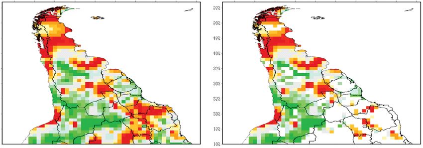
134                                                         F. de A. Diniz et al.

the state of Mato Grosso, Macapá in the state of Amapá,                  with maximum levels in summer and minimum in late
Recife in the state of Pernambuco, and Porto Alegre in                   winter.
the state of Rio Grande do Sul (Figure 2), the effect of                    Figure 4 refers to Brasília, located in Distrito Federal,
latitude on monthly temperature becomes clear, with                      showing a discrepancy of almost 180 degrees between
decreasing amplitudes from the south to the north of                     the curves of air relative humidity and evaporation.
Brazil. In Macapá, in the extreme north of the country,                  The humid summer, with monthly humidity averages
the monthly average temperature fluctuates slightly,                     of around 75%, limits evaporation to approximately
                                                                         100 mm per month, contrasting with the dry winter,
maintaining elevated average values throughout the
                                                                         with averages of around 50% and elevated evaporation
year, whereas in Porto Alegre, in the south of Brazil, a
                                                                         rates, which come close to 300 mm per month.
significant variation is observed from summer to winter.
                                                                            By comparing the climate normals for 1931–1960
The city of Cuiabá, located at an intermediate latitude,                 and 1961–1990 with the climate normals for 1981–
between both extremes, has more defined summers and                      2010, all published by Inmet, it is possible to have an
winters, which is also observed for Recife.                              idea of the climate variability among the three periods,
   Figure 3 illustrates the striking difference between
the rainfall regimes of four localities that are close in
terms of latitude: Salvador and Cuiabá, distant from
each other in terms of the climate factor continentality,
and Belém and Curitiba, located in extreme regions
of the country. Salvador, located on the coast, shows
higher accumulated precipitation, with maximum
precipitation in autumn and early winter, whereas
Cuiabá, a continental locality of the Midwestern
region of Brazil, presents scarcer rains, with maximum
levels at the end of spring and throughout summer.
In contrast, in Belém, located in the rainiest region
of the country and lying approximately at mean sea
                                                                         Figure 2. Comparison between the 1981–2010 climate
level, precipitation increases from December to June
                                                                         normals of compensated average temperature for Cuiabá in
and is practically consistent throughout the year, while                 the state of Mato Grosso, Macapá in the state of Amapá,
in Curitiba, located at about 1.000 m above mean sea                     Recife in the state of Pernambuco, and Porto Alegre in the
level, precipitation has a quite consistent distribution,                state of Rio Grande do Sul, Brazil. Source: Inmet (2018).

                                                                        Figure 3. Comparison between the 1981–2010 climate
Figure 1. Comparison of the 1981–2010 climate normals of                normals of the monthly accumulated precipitation for
atmospheric pressure at a station level for Belém in the state          Salvador in the state of Bahia, Cuiabá in the state of Mato
of Pará and Florianópolis in the state of Santa Catarina,               Grosso, Belém in the state of Pará, and Curitiba in the state
Brazil. Source: Inmet (2018).                                           of Paraná, Brazil. Source: Inmet (2018).

Pesq. agropec. bras., Brasília, v.53, n.2, p.131-143, Feb. 2018
DOI: 10.1590/S0100-204X2018000200001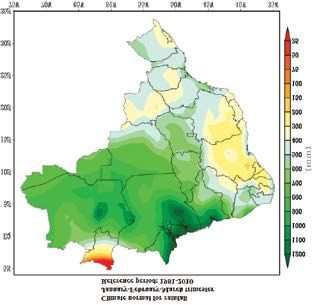
Brazilian climate normals for 1981–2010                                              135

as shown in Figures 5, 6, and 7. In Manaus, in the state         of Cuiabá in the state of Mato Grosso, Recife in the
of Amazonas, while the precipitation regime remained             state of Pernambuco, and Porto Alegre in the state of
stable and total precipitation slightly changed, with a          Rio Grande do Sul. This variable is very important,
small increase in August and December (Figure 5),                especially for the management and planning of water
the temperatures gradually increased about 1°C                   resources and of agricultural activities that require
throughout the year (Figure 6). However, in Goiânia, in          large amounts of water.
the state of Goiás (Figure 7), the average compensated              In this context, evaporation is one of the elements
temperature showed an increase of approximately                  that, aside from precipitation, characterize the
2°C, which should not be immediately interpreted as              climate of a region and have been widely used in
climate change associated with global warming, since             meteorological, climatological, and hydrological
                                                                 studies. It is possible to observe that Porto Alegre
it is more likely to be due to the effects of urbanization,
                                                                 presents a seasonal variation with low values, mainly
a hypothesis that will require more detailed studies.
                                                                 in the trimester May-June-July, whereas Recife shows
    Figure 8 presents an example of one of the new
                                                                 a smoothed variation throughout the year. Cuiabá
calculated variables, within a set of new parameters, for
                                                                 presents an elevated seasonal variation, mostly in the
the period of 1981–2010, i.e., the potential evaporation         second semester, indicating the maximum amount of
of regions with very different climates, in this case,           water that can evaporate from a soil covered entirely by
                                                                 vegetation, developed under optimum conditions and

Figure 4. Comparison between the 1981–2010 climate
normals of air evaporation and relative humidity for Brasília    Figure 6. Comparison between the 1981–2010, 1961–1990,
in Distrito Federal, Brazil. Source: Inmet (2018).               and 1931–1960 climate normals of average temperature for
                                                                 Manaus in the state of Amazonas, Brazil. Source: Inmet
                                                                 (2018).

Figure 5. Comparison between the 1981–2010, 1961–1990,
and 1931–1960 climate normals of the monthly accumulated         Figure 7. Comparison between the 1981–2010, 1961–1990,
precipitation for Manaus in the state of Amazonas, Brazil.       and 1931–1960 climate normals of average temperature for
Source: Inmet (2018).                                            Goiânia in the state of Goiás, Brazil. Source: Inmet (2018).

                                                                      Pesq. agropec. bras., Brasília, v.53, n.2, p.131-143, Feb. 2018
                                                                                        DOI: 10.1590/S0100-204X2018000200001
136 F. de A. Diniz et al.
assuming the absence of water availability limitations,
especially due to soil storage capacity.
In practical terms, the quantification of this variable
is a bit more complex, since it is affected by several
climatic factors, such as solar radiation, wind speed,
temperature, humidity, and local factors including
albedo, soil emissivity, and type of vegetation.
The historical average or climate normal may be
used, for example, to define the concept of “deviation”
or “anomaly” of a variable, often adopted in
meteorology to determine the difference between the
observed value and the corresponding climate normal.
Figure 8. Comparison between the 1981–2010 climate
normals of monthly potential evapotranspiration for Figure 9 illustrates the use of this concept in one of
Cuiabá in the state of Mato Grosso, Recife in the state of the products developed by Centro Regional del Clima
Pernambuco, and Porto Alegre in the state of Rio Grande para el Sur de América del Sur (CRS-SAS). CRS-
do Sul, Brazil. Source: Inmet (2018). SAS is an organization created in alignment with the
Figure 9. Deviation (anomaly) of the expected quarterly rainfall in relation to the 1981–2010 climate normals for the
trimester October-November-December of 2017 in the south region of South America. Source: CRS-SAS (2018).
Pesq. agropec. bras., Brasília, v.53, n.2, p.131-143, Feb. 2018
DOI: 10.1590/S0100-204X2018000200001Brazilian climate normals for 1981–2010 137
principles defined by WMO, which aims to provide days with machines in the field to the quantification
climate services in support of national meteorological of summer or wintering periods. Such information
services and other users from countries with part of is relevant for agriculture, livestock, urban life,
their territory located in the south region of South and many other human activities. The funding of
America. Using the climate normals for 1981–2010 as agricultural crops and general security activities
a reference, the Figure 9 shows precipitation anomalies are highly dependent on the knowledge of climate
predicted for the trimester October-November- conditions, particularly of extreme events, which can
December 2017, for the countries located in the be identified by the comparison of routinely observed
southeastern and southern regions of South America, meteorological conditions and by 10-day, monthly, and
with positive anomalies affecting mainly regions of annual averages.
Brazil, Argentina, and Paraguay. From another angle, the maps presented after the
The estimation of terms of climatological water respective tables allowed the spatial visualization
balance from temperatures and average monthly of the climatological information for a panoramic
rainfall data using the Thornthwaite (1948) and analysis and were useful tools for the decision making
Thornthwaite & Mather (1955) methods is an example process by authorities, planners, and executors of
of how climate information can be indirectly used for agrosilvopastoral activities, among others.
socioeconomic purposes, particularly for agriculture, The map in Figure 10, for example, illustrates
with graphical visualization of the data from the the accumulated annual rainfall normally expected
stations. On a 10-day scale, the greatest relevance throughout Brazil. If, for example, a given crop
lies in agricultural applications, particularly, in the requires accumulated annual rainfall higher than
selection of crops and agricultural practices that 1,500 mm, a farmer from the state of Minas Gerais
are more appropriate for a region. The comparison can only grow it in some areas of the Southern region
between the monitored real time and the average and of Triângulo Mineiro (in the west of the state of
10‑day values will allow the identification of favorable Minas Gerais), where such amounts are normally
or anomalous conditions for agricultural practices,
otherwise applicable to any other productive or social
activity. In particular, the 10-day water balance is an
essential tool in agricultural monitoring, especially
for the calculation of water deficit and potential and
real evapotranspiration, which are parameters that
allow quantifying the level of water stress to which
a crop is subjected to, besides estimating aridity and
productivity rates.
Temperature monitoring is also crucial in all
phenological stages of the crop, being a critical factor
in some processes such as, for example, flower abortion
in the coffee crop, when the plant’s tolerance limits are
exceeded in that phenological phase. Considering the
regional representativeness of each meteorological
station, a careful analysis of the normal monthly and
10-day values is of great importance in choosing:
varieties that are more suitable for a region, the best
seeding period, management and cultivation practices,
harvest processing activities, as well as other technical-
scientific and socioeconomic applications.
The statistics for number of rainy and dry days, and Figure 10. Climate normals of accumulated annual
for consecutive dry intervals are useful information precipitation (mm) for the period of 1981–2010 in Brazil.
for many activities, from the estimation of workable Source: Inmet (2018).
Pesq. agropec. bras., Brasília, v.53, n.2, p.131-143, Feb. 2018
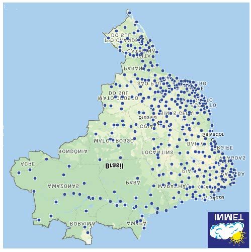
DOI: 10.1590/S0100-204X2018000200001138 F. de A. Diniz et al. obtained. Although other climate requirements must in that quarter, positive anomalies were recorded in the also be analyzed, especially temperature, this is a basic region, varying from 400 to 600 mm of accumulated analysis of agricultural zoning. rainfall, highlighting the relevance of the information The seasonal climate forecast illustrates another for agricultural activities and for the civil defense, important application of the quarterly climatological among other beneficiaries. average maps, which can be obtained from the sum Therefore, it is possible to carry out countless of the values of the normals for the months covered. analyses using tables and maps from the climate Since these forecasts are usually expressed in terms normals, depending only on the needs of the research of the probability of the occurrence of values above, to be developed. below, or within the climatological average, the map with the historical average for the period in question Methodology for calculating climate normals complements the information from the forecast. This allows to evaluate immediately and quantitatively The climate normals published here are averages from the value of the predicted parameter in any region of January 1, 1981, to December 31, 2010, corresponding interest, with its respective probability of occurrence. to Inmet’s network of 438 meteorological surface Figure 11 presents the forecast prepared by CRS-SAS stations in operation during that period (Figure 13). In using quarterly probabilistic forecasts for precipitation general, these are provisional normals, according to and also indicates a higher probability of occurrence of the concepts and procedures of WMO, established in above-average rainfall over the state of Santa Catarina. document WCDP No. 10 (WMO, 1989). When reading the climatological map of Figure 12, the user can verify that the average rainfall for this period Calculation procedures varies from 450 to 650 mm in the region, according to the climate normals for 1981–2010. In general, in order to determine the normals This forecast would, therefore, indicate that the of a variable for a given meteorological station, rainfall in these regions would likely score above it is necessary to initially calculate the Xij value this level in the first quarter of 2018, which in fact corresponding to each month i and each year j occurred according to subsequent verification. That is, belonging to the period of interest – in this case, 1981– Figure 11. Seasonal probabilistic forecast of accumulated precipitation: quarterly evaluation (A) and ≥0.3 Pearson correlation (B) for the trimester January–February–March of 2018, in the south region of South America. Source: CRS-SAS (2018). Pesq. agropec. bras., Brasília, v.53, n.2, p.131-143, Feb. 2018 DOI: 10.1590/S0100-204X2018000200001
Brazilian climate normals for 1981–2010                                              139

2010. WMO recommends that, in cases like these, the                                        X ij = ∑ X ijk
“3:5 rule” should be applied, discarding the months                                                k

with absence of data on 3 or more consecutive days, or              In these cases, WMO recommends that only full
5 or more alternate days.                                        months should be considered, that is, months with no
   For the variables of Group I associated with daily values,    missing data.
such as temperature, atmospheric pressure at a station              A particular case is the calculation of 10-day
level and at mean sea level, vapor pressure, air relative        precipitation for the first, second, or third 10 days of
humidity, cloudiness, and wind, Xij is computed as:              each month. The 10-day value is calculated by the sum
                                                                 of the daily values for the days in question. It should
                     X ij = ∑ X ijk N
                            k
                                                                 be noted that, according to WMO guidelines, only
                                                                 complete periods of 10 days – with no missing data –
where Xijk is the observed value of variable X on day
                                                                 should be considered.
k, of month i, of year j; and N is the number of days in            The variables of Group III represent events observed
month i, of year k, for which observations are available.        in a period of interest, such as a month or a determined
   For the calculation of vapor pressure, the Tetens             10 days of a month. Examples are days with rainfall
equation was used:                                               or temperature above a certain threshold, or periods
      es = A × exp17.3t/23.7 + t or es = A × 107.5t/237.3 + t    with consecutive days without rainfall, within a month
where the parameter A corresponds to 610.8 Pa (for               or in a given 10 days of the month. In these cases,
results in Pa) or 0.6108 kPa (for results in kPa), and t is      the variable corresponds to the total of observations
the temperature given in Celsius (°C).                           recorded in month i, of year j. As an example, take
   For the variables of Group II associated with                 the number of days with rainfall higher or equal to 1
accumulated values in the period of interest, such               mm in the first 10 days of a month: if i corresponds
as precipitation, evaporation, and insolation, Xij is            to the month of March, and j to the year of 1975, then
calculated as the accumulated value in month i of year           Xij will correspond to the total number of days with
j, namely, as the sum of all available daily values for
that month and that year:

Figure 12. Historical average of the accumulated
precipitation in the trimester January–February–March of         Figure 13. Spatial distribution of the 411 meteorological
2018, in Brazil, using the climate normals for 1981–2010 as      stations in Brazil, recalculated for the period of 1981–2010.
a reference. Source: Inmet (2018).                               Source: Inmet (2018).

                                                                      Pesq. agropec. bras., Brasília, v.53, n.2, p.131-143, Feb. 2018
                                                                                        DOI: 10.1590/S0100-204X2018000200001
140 F. de A. Diniz et al.
rainfall, meeting that condition during the first 10 regression equations of temperature versus altitude,
days of March 1975. Again, following the procedures latitude, and longitude; when applied for periods
recommended by WMO, the observation period longer than 10 days, its estimates are reasonable.
should be complete, i.e., only months with rainfall data In the case of the variables of Group I, the annual
available for every single day should be considered normal ( X ) of variable X in the meteorological station
for the 10-day average and only the month that has in question is calculated as the average of the X i 12
rainfall data for every single day should be taken monthly values, i= 1, ...,12. For the variables of Groups
into account for days with rainfall in a certain month. II and III, the annual normal X will be calculated as
For variables in any of the three groups, the normal the sum of the 12 monthly values. If there is no X i for
corresponding to month i will then be calculated as: any of the 12 months of the year, the annual amount
will not be calculated.
X i = ∑ X ij mi
j
where mi is the number of years for which Xij values Calculation of daily values
are available. Data collection at Inmet’s conventional
According to WMO’s nomenclature, if mi is equal meteorological stations is carried out at 12:00, 18:00,
to 30, starting on January 1, 1961, and ending on and 24:00 UTC. However, in a few stations, the
December 31, 1990, X i will be a standard normal or observations are carried out only twice a day, usually
standardized. If mi is lower than 10 but equal to or at 12:00 and 24:00 UTC.
greater than 10, X i will be a provisional normal. In The Xijk daily values used in the calculations
case mi is lower than 10, the X i value will be discarded. described above result from these observations,
The potential evapotranspiration corresponds to the according to the rules summarized hereinafter.
maximum water capacity that can be lost as vapor in The minimum and maximum daily temperatures
a given climate condition by a continuous vegetation are recorded in special thermometers (maximum-
covering the entire surface, whether at or above field minimum thermometer) and read by the observer,
capacity. This includes soil evaporation and vegetation usually at 12:00 and 24:00 UTC, respectively.
transpiration in a specific region and in a given time The average compensated temperature, used in this
interval. The potential evapotranspiration (ETp, in publication, is calculated by the formula:
mm per month) was indirectly calculated using the
TMC,ijk = (Tmax,ijk + Tmin,ijk + T12,ijk + 2T24,ijk ) / 5
Thornthwaite method (1948), based on the correlation
between measured evapotranspiration and air For the calculation of the daily value of air relative
temperature data, according to the following empirical humidity, Inmet also uses the compensated average
method: value given by:
ETp = b×(Tm)a
UR C,ijk = ( UR12,ijk + UR18,ijk + 2 UR 24,ijk ) / 4
where
a = (67.5x10⁻⁸×I3) - (7.71x10⁻⁶×I2) + (0.01791×I) + For the other variables of Group I, namely,
0.492; atmospheric pressure, cloudiness, and wind direction
I = ∑112(Tmi/5)1.514 (sum of the 12 months of the year); and intensity, the daily value is calculated by the
B = (N/12), day length adjustment factor; simple arithmetic mean of the values recorded in the
N is the maximum daily insolation, latitude, and three observation times. When one of these data sets
month function; I is the heat index; and Tm is the is missing, it is not possible to obtain a daily value
average daily temperature. for these variables, or for the compensated average
The Thornthwaite (1948) method, as an empirical temperature and the compensated air relative humidity.
formula, loses accuracy especially when applied at a In the case of the variables of Group II, i.e.,
daily scale. However, it is still one of the most adopted precipitation, evaporation, and insolation, the daily
methods because it only uses air temperature, whose values are calculated as accumulated totals throughout
monthly and annual averages can be estimated even the day, measured at 12:00 UTC (9 hours from Brasília
for regions without climate information through at a standard time or 10 hours during daylight saving
Pesq. agropec. bras., Brasília, v.53, n.2, p.131-143, Feb. 2018
DOI: 10.1590/S0100-204X2018000200001Brazilian climate normals for 1981–2010 141
time). Therefore, for example, the value of rain of occurrence of the normal value of 0.3, mentioned
associated with today will correspond to the total above, can be estimated as 3/20 or 15%. As a general
accumulated rainfall from 12:00 UTC of yesterday rule, the probability, in percentage values, can be
until 12:00 UTC of today. estimated as:
Probability [Normal Value = x] = (x / Max_Num_
Days with or without rainfall Dry_Days) * 100
where Max_Num_Dry_Days is the maximum number
To count the days with or without rainfall in a month or of dry days that can be observed in a typical month.
a period of 10 days, the two following recommendations The reference values for 5 or more and 3 or more
of WMO were taken into consideration: 1, using only consecutive dry days are, respectively, 5.0 and 7.6
periods with complete data, that is, months or 10-day (approximately). In order to facilitate the interpretation
periods with precipitation data registered daily; and 2, of the values presented in the tables and map subtitles
considering days with or without rainfall as those in referring to the number of periods with 3 or more,
which accumulated precipitation was higher or equal/ 5 or more, and 10 or more consecutive dry days,
lower than 1 mm. frames that are presented in the introductory pages of
Being, by definition, an integer variable, when the the maps were produced, being equally valid for the
normals for number of days with rainfall in a month (or
interpretation of the respective tables.
a year) were calculated, the fractional values obtained
were rounded to the nearest integer. However, since the Wind at 10 m
loss of information deriving from the rounding would
be much more significant in terms of percentage for 10- Wind intensity was treated as a normal variable
day averages, these were expressed with one decimal of Group I. Furthermore, the hourly values of wind
point, leaving the user with the task of transforming intensity were analyzed in zonal (variable u) and
them into integer values, whenever convenient. meridional (variable v) components. The daily value
of these variables was calculated as the mean of the
values of the three measurement times, and the climate
Periods of consecutive dry days
normal of these quantities was, then, calculated by the
The aforementioned rounding does not apply, standard rules of Group I.
however, to the case of number of periods with 3 or Figure 14 illustrates the definitions of wind speed,
more, 5 or more, and 10 or more consecutive days θ, and the zonal (u) and meridional (v) components
without rain. The interpretation of the obtained values, used in meteorology. In this paper, wind direction
in this case, becomes easier if translated in terms of was addressed in two complementary forms. The first
number of observed events, on average, for a period of consisted of the direct calculation of the value resulting
10 or 30 years or in terms of the probability (relative from wind direction using the following expression:
frequency) of the event at hand occurring. Take, for
example, the case of number of periods with 10 or |tan-1(n(v)/n(u)) - 270º|, if n(u) > 0
more consecutive dry days. Suppose that, for a given n(θ) =
locality and for a given month of the year, a normal |tan-1(n(v)/n(u)) - 90º|, if n(u) < 0
value of 0.3 was obtained. This is to say that 3 events where the counter-domain of the arc tangent function,
would be observed on average over a period of 10 tan-1(x), is the interval (-0º, 90º) and n(u) and n(v)
years or 30 events in 30 years. To translate this result represent the climate normals of the zonal and
in terms of probability (or relative frequency), it is meridional components, respectively.
necessary to compute the maximum number of events The second form consisted in collecting, for each
that could be observed in a typical month. It is easy station and each month of the year, the prevailing
to verify that, at any given month of the year, only direction of the wind. To this end, the relative
a maximum of two distinct periods with 10 or more frequencies were obtained for the wind originating
consecutive dry days would be possible. Therefore, in from eight main directions, namely: north (N),
10 years, a maximum of 20 events could be observed northeast (NE), east (E), southeast (SE), south (S),
in the month in question. In this case, the probability southwest (SW), west (W), and northwest (NW).
Pesq. agropec. bras., Brasília, v.53, n.2, p.131-143, Feb. 2018
DOI: 10.1590/S0100-204X2018000200001142 F. de A. Diniz et al.
For this purpose, every hourly measurement of wind Concluding remarks
direction referring to the month in question, available
at the station for the period of 1961–1990, was The new version of the 1981–2010 Brazilian
categorized in the eight ranges of direction previously climate normals will be available at Inmet’s webpage
specified. Thereafter, the band (direction) of highest ( http://www.inmet.gov.br/portal/index.php?r=clima/
normaisClimatologicas). It will contain maps and Excel
relative frequency was determined, subject to the
sheets corresponding to all parameters, as well as
restriction that this frequency was higher than 20%.
explanatory texts that can provide the information
Whenever this condition was not met, the prevailing
necessary for the desired research. In case there is
direction was considered indefinite (INDEF).
no information on your city, it is possible to analyze
nearby cities, which can be used as references.
Final adjustments As in any complex work, the results consolidated
Rule of 10 in this paper are naturally prone to error and
The values of the climate normals resulting from improvements and, therefore, always subject to
the analysis described in the previous section were criticism. The executing team strived for the best
subjected to a filter: a minimum of 10 years of possible product, within limitations of time and
available data in the Weather Information System available resources. However, we are certain that the
(SIM) for each station combination, meteorological user community of the information presented here
variable, and month under consideration. As will now have at their disposal a more complete and
improved product. Certainly, new updates will be
explained before, this condition is required by
produced by Inmet in a near future, focusing on other
WMO for a provisional normal. Thereafter,
periods such as 1971–2000 and 1991–2000, since
for each variable, those stations that only had
WMO advocates that the climate normals should be
climatological averages for a number of months
calculated in consecutive periods of 30 years (1901–
inferior to 10 were also discarded.
1930, 1931–1960, 1961–1990, 1991–2020…). However,
the calculation of intercalated periods, like 1971–2000,
has also become a common practice as done by National
Oceanic and Atmospheric Administration (NOAA). It
is hoped that, with the accumulated experience, future
products will be increasingly better. This is a natural
process of evolution, which, in no way, diminishes past
achievements when theoretical shortcomings and the
absence of computational resources required greater
dedication and efforts from the preceding teams.
References
BRASIL. Departamento de Meteorologia. Normais
climatológicas 1961-1990. Rio de Janeiro: Ministério da
Agricultura e Reforma Agrária, 1992. 91p.
BRASIL. Departamento de Meteorologia. Normais
climatológicas: área do Nordeste do Brasil: período 1931-1960.
Rio de Janeiro: Ministério da Agricultura, 1970. 91p.
CRS-SAS. Centro Regional del Clima en red para el Sur de
América del Sur. Diagnostico y perspectivas climáticas. [S.l.],
2018. Available at: ˂http://www.crc-sas.org/pt/perspectivas_
Figure 14. Diagram illustrating the definition of the angle climaticas.php˃. Accessed on: Feb. 28 2018.
that determines wind direction and decomposition in zonal INMET. Instituto Nacional de Meteorologia. [Normais
(u) and meridional (v) components, for two wind vectors Climatológicas do Brasil 1981-2010]. Brasília, 2018. Available
of intensities I0 and I1 and directions θ0 (northeast) and θ1 at: ˂http://www.inmet.gov.br/portal/index.php?r=clima/
(southeast). N, north; E, east; S, south; and W, west. normaisClimatologicas˃. Accessed on: Feb. 28 2018.
Pesq. agropec. bras., Brasília, v.53, n.2, p.131-143, Feb. 2018
DOI: 10.1590/S0100-204X2018000200001Brazilian climate normals for 1981–2010 143
PACHAURI, R.K.; MEYER, L.A. (Ed.). Climate Change 2014: THORNTHWAITE, C.W.; MATHER, J.R. The water
synthesis report. Geneva: IPCC, 2014. 151p. Contribution of balance. Centerton: Drexel Institute of Technology,
Working Groups I, II and III to the Fifth Assessment Report of Laboratory of Climatology, 1955. 104p. (Publications in
the Intergovernmental Panel on Climate Change. Climatology, v.8).
RAMOS, A.M.; SANTOS, L.A.R. dos; FORTES, L.T.G. (Org.). WMO. World Meteorological Organization. Calculation of
monthly and annual 30-year standard normals. [Washington]:
Normais climatológicas do Brasil 1961–1990. Brasília: INMET, 2009.
World Meteorological Organization, 1989. (World Climate Data
THORNTHWAITE, C.W. An approach toward a rational Programme. WCDP n.10; World Meteorological Organization.
classification of climate. Geographical Review, v.38, p.55-94, 1948. WMO-TD n. 341).
Received on January 4, 2018 and accepted on February 21, 2018
Pesq. agropec. bras., Brasília, v.53, n.2, p.131-143, Feb. 2018
DOI: 10.1590/S0100-204X2018000200001You can also read