Direct measurements of atomic oxygen in the mesosphere and lower thermosphere using terahertz heterodyne spectroscopy - DLR
←
→
Page content transcription
If your browser does not render page correctly, please read the page content below
ARTICLE
                  https://doi.org/10.1038/s43247-020-00084-5                 OPEN

                  Direct measurements of atomic oxygen in the
                  mesosphere and lower thermosphere using
                  terahertz heterodyne spectroscopy
                  Heiko Richter1, Christof Buchbender 2, Rolf Güsten3, Ronan Higgins2, Bernd Klein3, Jürgen Stutzki2,
                  Helmut Wiesemeyer3 & Heinz-Wilhelm Hübers 1,4 ✉
1234567890():,;

                  Atomic oxygen is a main component of the mesosphere and lower thermosphere of the Earth,
                  where it governs photochemistry and energy balance and is a tracer for dynamical motions.
                  However, its concentration is extremely difficult to measure with remote sensing techniques
                  since atomic oxygen has few optically active transitions. Current indirect methods involve
                  photochemical models and the results are not always in agreement, particularly when
                  obtained with different instruments. Here we present direct measurements—independent of
                  photochemical models—of the ground state 3P1 → 3P2 fine-structure transition of atomic
                  oxygen at 4.7448 THz using the German Receiver for Astronomy at Terahertz Frequencies
                  (GREAT) on board the Stratospheric Observatory for Infrared Astronomy (SOFIA). We find
                  that our measurements of the concentration of atomic oxygen agree well with atmospheric
                  models informed by satellite observations. We suggest that this direct observation method
                  may be more accurate than existing indirect methods that rely on photochemical models.

                  1 German Aerospace Center (DLR), Institute of Optical Sensor Systems, Rutherfordstraße 2, 12489 Berlin, Germany. 2 I. Physikalisches Institut der Universität

                  zu Köln, Zülpicher Straße 77, 50937 Köln, Germany. 3 Max-Planck-Institut für Radioastronomie, Auf dem Hügel 69, 53121 Bonn, Germany. 4 Department of
                  Physics, Humboldt-Universität zu Berlin, Newtonstraße 15, 12489 Berlin, Germany. ✉email: heinz-wilhelm.huebers@dlr.de

                  COMMUNICATIONS EARTH & ENVIRONMENT | (2021)2:19 | https://doi.org/10.1038/s43247-020-00084-5 | www.nature.com/commsenv                                     1
ARTICLE COMMUNICATIONS EARTH & ENVIRONMENT | https://doi.org/10.1038/s43247-020-00084-5
A
tomic oxygen extends from about 80 km to above 300 km understanding the photochemistry and the energy budget of the
in altitude, but with more than 90% concentrated between MLT.
85 and 125 km (Fig. 1a). It plays an important role for the At the atmospheric conditions of the MLT the fine structure
energy balance of the mesosphere and lower thermosphere line at 4.7448 THz is thermally Doppler broadened with a line
(MLT), because it participates in exothermic chemical reactions width of ∼12 MHz for emission originating at ∼100 km where the
and it contributes to radiative cooling1,2. The latter occurs mainly density of atomic oxygen is largest. Due to the increasing tem-
via emission from CO2 at 15 µm and NO at 5.3 µm. Both mole- perature, emission from the thermosphere is broader (∼25 MHz
cules are excited by collisions with ground state atomic oxygen. In at altitudes >300 km). Direct observation of this transition
particular, quenching of CO2 vibrational levels by collisions with requires airborne or space-borne instruments, because absorption
atomic oxygen is important. Therefore, the knowledge about the by tropospheric water vapor prohibits observation with ground-
distribution of atomic oxygen is crucial for retrieval of the kinetic based instruments. In addition, terahertz (THz) spectrometers are
temperature in the MLT from the 15 µm CO2 radiance3. In notoriously complex, in particular when it comes to airborne or
addition, direct radiative cooling by atomic oxygen occurs via the space-borne applications. The 4.7-THz line has been observed a
fine structure transition from the lowest excited state, 3P1, into few times by rocket-borne instruments8. More observations with
the ground state, 3P2, at 63.2 µm (4.7448 THz)4. This is the global coverage have been done with the Cryogenic Infrared
dominant cooling mechanism above ~250 km. In the MLT the Spectrometers and Telescopes for the Atmosphere (CRISTA) that
lifetime of atomic oxygen in the 3P1 state is several hours. Because flew on the space shuttle in the 1990s9,10. With this spectrometer
of this long lifetime it can be transported over large distances atomic oxygen densities have been determined at altitudes from
before it releases its energy and therefore it might be used as 130 to 175 km, which account for about 20% of the total atomic
tracer for the dynamical motions, vertical transport, tides, and oxygen in the MLT. Below 130 km retrieval was not possible,
winds5–7. This leads to a strong coupling between the dynamics because of the opacity of the transition and the limb view of
and the photochemistry in the MLT with the energy being CRISTA. Measurements of the fine-structure line have also been
released significantly after and far away from the location, where made with the Far-InfraRed Spectrometer (FIRS-2), a Fourier
the UV photon is absorbed. An accurate knowledge of the global transform spectrometer on a high-altitude (∼38 km) balloon11.
distribution of atomic oxygen and its concentration profile as well From 1989 to 2003 in total 31 spectra have been obtained and
as diurnal and annual variations are therefore essential for analyzed. But again, the line shape of the transition was not
Temperature (K)
100 200 300 400 500 600 700 800 900
400 c
50°
300 a
Altitude (km)
9607 s
200 C
8236 s
Temperature
7885 s
100 Atomic oxygen
B
70 40°
1E8 1E9 1E10 1E11 1E12
Atomic oxygen concentration (cm-3) 5746 s
1.2
1.0
4968 s
b CRISTA
Normalized signal (arb. u.)
1.0
0.5
0.8
0.0 2617 s
0.6 4.72 4.73 4.74 4.75 4.76
2202 s
0.4
30°
FIRS-2
0.2
0s A
-120°
-130°
0.0 GREAT
4.7442 4.7444 4.7446 4.7448 4.7450 4.7452 4.7454
Frequency (THz)
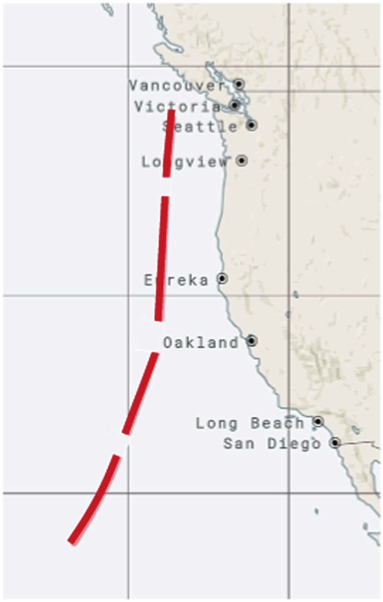
Fig. 1 Atomic oxygen observation with GREAT on SOFIA. a Concentration profile of atomic oxygen and temperature measured by the SABER instrument
(blue squares) at altitudes ranging from 80 to 100 km. The straight red and blue lines are calculated profiles with NRLMSISE-00 (at position B in Fig. 1c).
b Comparison of the spectra measured with the grating spectrometer of CRISTA (black line in the inset), with the balloon-borne FIRS-2 Fourier transform
spectrometer (blue line) and with the GREAT heterodyne spectrometer (red line). Only with GREAT the atomic oxygen line is spectrally resolved.
c Trajectory of the SOFIA flight (red line) where the spectra have been acquired between 1:15 and and 4:15 am on 14 January 2015. The numbers along
the trajectory indicate the flight time in seconds. Short interruptions are due to a reorientation of the telescope. The white circles mark the positions where
the spectra of Fig. 2 have been measured (A: 50.6°, 1:21 am; B: 38.3°, 3:11 am; C: 29.1°, 4:01 am). The dashed blue line indicates the flight trajectory of
SABER. The red dots and blue squares in 1a are an average of nine profiles measured with SABER along the flight track between the two blue stars in 1c on
14 January 2015 between 0:22 and 0:30 am local time (Map: © Open Street Map contributors, https://www.openstreetmap.org/copyright).
2 COMMUNICATIONS EARTH & ENVIRONMENT | (2021)2:19 | https://doi.org/10.1038/s43247-020-00084-5 | www.nature.com/commsenvCOMMUNICATIONS EARTH & ENVIRONMENT | https://doi.org/10.1038/s43247-020-00084-5 ARTICLE
resolved. The radiances observed by FIRS-2 deviate by less than time of 1 s. With this sensitivity GREAT is capable of measuring
15% from the computed ones using the Mass Spectrometer one spectrum with an integration time of 19 s. For comparison,
Incoherent Scatter (MSIS) model11,12. 31 separate spectra have been measured with FIRS-2 each
Atomic oxygen concentrations can be inferred indirectly from requiring between 11 and 16 min of integration time. It should be
measurements of the O(1S) green line, the O2 A-band or the noted that GREAT is a rather large instrument, which, in its
emission from vibrationally excited OH. These methods rely on present form, cannot be implemented on a balloon or on a
chemical reaction models and assumptions such as photo- satellite. However, recent improvements in heterodyne technol-
chemical steady state, quenching rates, radiative lifetimes, and ogy, in particular high-frequency Schottky diode mixers26, com-
reaction coefficients. The OH emission has been measured with pact quantum-cascade lasers as local oscillators27, and low-power
the SABER (Sounding of the Atmosphere using Broadband CMOS (Complementary Metal-Oxide Semiconductor) backend
Emission Radiometry) infrared spectrometer and with the Scan- spectrometers28 have initiated the development of balloon-borne
ning Imaging Absorption Spectrometer for Atmospheric Char- and satellite instruments29,30.
tography (SCIAMACHY)6,13,14. The O(1S) green line was The spectra, which are presented here, have been measured on
measured by the Wind Imaging Interferometer (WINDII) and 14 January 2015 between 1:15 and 4:15 am (flight ID 2015/01/14).
SCIAMACHY instruments15–17 and the O2 A-band airglow has The flight trajectory is shown in Fig. 1c. Essentially it is in south-
been measured with SCIAMACHY and the Optical Spectrograph north direction above the Pacific Ocean west of northern Mexico
and InfraRed Imaging System (OSIRIS) on the Odin satellite18. and California between 27° and 48° north latitude and 134° and
With all instruments geographical and seasonal variations of the 128° west longitude. The flight direction is from south to north
atomic oxygen concentration have been found. Initially, differ- and the telescope is viewing west. Three typical profiles obtained
ences up to 60% are reported for concentrations derived from OH during this flight are shown in Fig. 2. They have been measured at
measurements with SABER and O(1S) measurements with three different elevations, as well as at different locations along
SCIAMACHY16. A recent comparison based on an improved the flight track and different altitudes. The measurement uncer-
photochemical model reveals differences up to 20% between tainty in intensity is ±15%. It is caused by uncertainties of the
SABER, SCIAMACHY, WINDII, and OSIRIS measurements19. absorption by water vapor and calibration uncertainties (see
The new atomic oxygen concentrations are about 25% smaller “Methods” section). At the lowest elevation of 29.1° the profile is
than those originally derived19,20. Likewise, with an improved the broadest with signs of saturation as the flat top indicates.
photochemical model it was found that the atomic oxygen con- With increasing elevation it becomes narrower and at the largest
centrations derived from OH, O(1S), and O2 A band measure- elevation of 50.6° saturation almost disappears, because the path
ments with SCIAMACHY agree within 15% with each other, through the atmosphere becomes shorter and less atomic oxygen
which is better than the agreement with SABER data derived from is probed. It should be noted that most of the signal in the wings
OH measurements21. of the profile is from altitudes around 100 km. The red solid lines
are radiative transfer calculations based on atomic oxygen column
densities and temperature profiles from NRLMSISE-00 (US Naval
Results and discussion Research Laboratory Mass Spectrometer and Incoherent Scatter
Direct observations of atomic oxygen are potentially more Radar Exosphere − 2000)31. Each line profile is a convolution
accurate. We have analyzed its emission at 4.7 THz measured with the 6 MHz spectral resolution of the GREAT spectrometer.
with the GREAT spectrometer on SOFIA, the Stratospheric The elevation of the telescope as well as the absorption by the
Observatory for Infrared Astronomy22,23. This is a by-product of atmosphere between SOFIA and the MLT are also taken into
the astronomical observations in the same frequency band. In account (see “Methods” section). The residuals (modeled minus
fact, atomic oxygen has been observed in the atmosphere of Mars measured data) are up to 15% and the largest deviations occur in
using GREAT24. Due to Doppler shift the line from the astro- the wings of the profiles, indicating that the atomic oxygen
nomical object is often significantly shifted (up to ∼3 GHz) from concentration is somewhat different from the model in particular
the atmospheric line. This allows analyzing the spectra of the at higher altitudes.
atomic oxygen line in the Earth atmosphere for those astro- In order to analyze the accuracy of the model we have calcu-
nomical objects, which are significantly Doppler shifted and not lated the emission profiles assuming various deviations from the
too much broadened, ensuring that the lines do not interfere. atomic oxygen concentration and temperature profiles of
Heterodyne spectroscopy has a number of differences com- NRLMSISE-00 (Fig. 3). First, we have varied the concentration
pared to grating spectroscopy and Fourier-transform spectro- profile from 120 to 80% of the nominal concentration at all
scopy regarding the measurement of atomic oxygen in the altitudes. The residuals show that the best agreement is obtained
atmosphere. First of all it provides a much higher spectral reso- with the nominal concentrations from NRLMSISE-00. It should
lution. In the case of GREAT the spectral resolution of ∼6 MHz be noted that the residuals become more pronounced in the wings
(full width at half maximum (FWHM), see “Methods” section) is of the profile while the peak remains unchanged because of
limited by the line width of the local oscillator (LO)25. This is saturation. This underlines the importance of the high spectral
significantly smaller than the atomic oxygen line width. In resolution. When the temperature, T, is changed by ±5% while
comparison, CRISTA has a spectral resolution of ∼4.2 GHz8 and the concentration profile is kept nominal the emission becomes
FIRS-2 has 120 MHz spectral resolution11. The resolving power of much stronger (T = +5%) or much weaker (T = −5%), because
GREAT allows spectrally resolving the atomic oxygen line more or less atomic oxygen is excited. An important difference to
(Fig. 1b). Because of the high spectral resolution the problem of the residuals for different atomic oxygen concentrations is that in
saturation of the atomic oxygen line can be overcome in the this case the residual at the peak of the line changes significantly.
vertical sounding observation geometry of GREAT (see “Meth- In Fig. 3c calculated profiles are shown which are obtained by
ods” section). This occurs in the center of the line while the line shifting the concentration profile by +5 km or −5 km relative to
wings are not saturated and contain information about the atomic the nominal profile while keeping the temperature profile
oxygen concentration at higher altitudes. The second advantage is unchanged. Again, the deviation from the measured profile is
the high sensitivity of the GREAT spectrometer. Its single- pronounced. When the concentration profile is shifted by −5 km
sideband noise temperature is 2200 K. This corresponds to a noise a single peak occurs and saturation of the emission is reduced. A
equivalent power (NEP) of 3 × 10⁻²⁰ W within an integration double-peak emission profile appears when the concentration
COMMUNICATIONS EARTH & ENVIRONMENT | (2021)2:19 | https://doi.org/10.1038/s43247-020-00084-5 | www.nature.com/commsenv 3ARTICLE COMMUNICATIONS EARTH & ENVIRONMENT | https://doi.org/10.1038/s43247-020-00084-5
0.7 a b c
Signal (pW Hz-1 m-2 sr -1)
0.6 50.6° 38.3° 29.1°
0.5
0.4
0.3
0.2
0.1
0.0
0.1
e f
Residual
d
0.0
-0.1
4.74475 4.74480 4.74475 4.74480 4.74475 4.74480
Frequency (THz) Frequency (THz) Frequency (THz)
Fig. 2 Emission spectra of atomic oxygen at different elevation of the telescope. a–c Typical spectra of atomic oxygen measured at 50.6°, 38.3°, and
29.1° (black lines, flight altitude: approx. 13 km). The red lines are radiative transfer calculations based on NRLMSISE-00. d–f Residuals of the measured and
calculated profiles (black lines). With decreasing elevation the saturation of the profile increases, because of the longer optical path through the
atmosphere. The positions where the spectra have been measured are marked in Fig. 1c.
0.8
a b c
0.7 measured measured measured
Signal (pW Hz-1 m-2 sr-2)
120% OI nominal nominal
0.6 100% OI T+5% +5 km
80% OI T -5% -5 km
0.5
0.4
0.3
0.2
0.1
0.0
Residual
0.1 d e f
0.0
-0.1
4.74475 4.74480 4.74475 4.74480 4.74475 4.74480
Frequency (THz) Frequency (THz) Frequency (THz)
Fig. 3 Dependence of the atomic oxygen emission profile on concentration, temperature and height. a–c Measured spectrum (black line) of atomic
oxygen at 38.3° elevation (same spectrum as in Fig. 2) with several fits (blue, red, and green lines) based on concentration profiles and temperature
profiles from NRLMSISE-00. a Atomic oxygen concentration is 120 or 80% of the nominal value (100%). b The temperature profile has been changed by
±5%. In this case large deviations occur at the peak of the line. c The peak of the nominal concentration profile is shifted by ±5 km. Again, large deviations
occur at the peak. d–f The smallest residuals are obtained with the nominal 100% concentration and the largest deviations are in the wings of the line while
the peak is not much affected.
profile is shifted upwards, because the wings of the emission and 0:30 am local time19. (ftp://saber.gats-inc.com/Version2_0/
profile are less attenuated. They probe higher atmospheric layers SABER_atox_Panka_etal_2018_GRL/SABER_o3p_oh_night_
and more atomic oxygen contributes to the signal. 2015_v1.0.nc). The profiles extend from 80 to 100 km altitude.
Because NRLMSISE-00 is not a physics-based model, an Since there are no measured data available for altitudes above
agreement between this model and the GREAT measurements 100 km we have combined SABER and NRLMSISE-00 atomic
might be accidental. Therefore we compare the GREAT data with oxygen and temperature profiles. Below 100 km these consist of
atomic oxygen profiles obtained with the SABER instrument. the SABER profile while above 100 km the NRLMSISE-00
There is a set of nine SABER profiles, which was measured profiles were taken. With these concentration and temperature
close to the geolocation and time of the GREAT measurements profiles the expected atomic oxygen emission is calculated
(see “Methods” section). This data has been measured along the and compared with the measured emission (position B in
flight track shown in Fig. 1c on 14 January 2015 between 0:22 Fig. 1c). The agreement between the GREAT and the SABER/
4 COMMUNICATIONS EARTH & ENVIRONMENT | (2021)2:19 | https://doi.org/10.1038/s43247-020-00084-5 | www.nature.com/commsenvCOMMUNICATIONS EARTH & ENVIRONMENT | https://doi.org/10.1038/s43247-020-00084-5 ARTICLE
0.8
a
0.7 GREAT
Signal (pW Hz-1m-2sr-1)
SABER 400
0.6
300 GREAT (1σ)
0.5
c SABER
NRLMSISE-00
0.4
Altitude (km)
200
0.3
0.2
0.1
100
0.0 90
80
70
b
Residual
0.1
60
0.0 50
1E8 1E9 1E10 1E11 1E12
-0.1
Atomic oxygen concentration (cm-3)
4.74470 4.74475 4.74480 4.74485
Frequency (THz)
Fig. 4 Atomic oxygen emission and concentration profile. a Emission profile measured with GREAT (black line, position B in Fig. 1c) and calculated
emission profile (red line) from combined SABER/NRLMSISE-00 atomic oxygen and temperature profiles. b Residual (black line) of the measured and
calculated profiles shown in a. c Combined SABER (red squares) and NRLMSISE-00 (straight red line) profile. The grey area indicates those profiles which
are compatible with the measured GREAT spectrum (±1σ uncertainty).
NRLMSISE-00 profiles is similar as with the pure NRLMSISE- Elevation (°)
00 profiles (Fig. 4a). The differences are within the uncertainty 50.5 45.7 41.0 36.7 32.7 40.0 36.5 32.8 29.1
of the GREAT measurement. Also, day-to-day variations of 2.4
atomic oxygen and temperature as well as uncertainties of the a
2.2
Radiance (nW cm-2 sr-1)
SABER data and NRLMSISE-00 may contribute to the differ-
ences. An analysis of the altitude profiles is shown in Fig. 4b.
2.0
Along with the combined SABER/NRLMSISE-00 profiles it
displays a range (±1σ) of atomic oxygen concentration profiles,
1.8
which are compatible with the GREAT spectra. At the peak this
is an uncertainty of approx. ±40%. The range of profiles is 1.6
derived by varying the atomic oxygen concentration profile, the
temperature profile and the relative positon of both starting 1.4
with the best fit NRLMSISE-00 profile. The variations of these
parameters were determined, which provide residuals of less 1.2
Norm. Radiance
than the measurement uncertainty of ±15%. The combined 1.2
SABER/NRLMSISE-00 profile falls into this range. b
We now turn to the analysis of the flight path in Fig. 1c with 1.0
254 spectra. For each spectrum the radiance has been determined 0.8
by integration of the emission profile and plotted as a function of 0 2000 4000 6000 8000 10000
flight time (Fig. 5). All data are corrected for absorption by Time (s)
atmospheric water vapor, which is determined by fitting the
Fig. 5 Radiances measured along the flight path of SOFIA. a Measured
maximum of the saturated emission profiles (see “Methods”
(red dots) and calculated (straight red line) radiances along the flight path
section). In contrast to Fig. 2a single value for the precipitable
shown in Fig. 1c (bottom scale: time of flight, top scale: elevation of the
water vapor (pwv) content has been applied to all spectra (see
telescope). The measured data are corrected for absorption by atmospheric
“Methods” section). The calculated radiances take into account
water vapor using the same pwv value for all data. The straight line has
the atomic oxygen concentration and temperature profiles from
been calculated with the NRLMSISE-00 model taking into account the
NRLMSISE-00 and the elevation of the telescope. It should be
elevation of the telescope. Data obtained from 254 spectra are plotted.
noted that along the flight path the atomic oxygen concentration
The radiance increases until t = 5000 s and from t = 6000 s onwards,
as well as the temperature predicted by NRLMSISE-00 change by
because the elevation of the telescope decreased from ∼51° to ∼32° (until
less than ±5% at all altitudes between 50 and 400 km. If only the
5000 s) and from ∼42° to ∼29° (from 6000–10,000 s). The interruption
region with the highest concentration of atomic oxygen is con-
between 5000 and 6000 s corresponds to a reorientation of the telescope.
sidered (85–125 km) the changes are less than ±2%. The mea-
b Normalized radiance (black dots, measured radiance divided by
sured radiances agree with the calculated ones within the
calculated radiance) during flight. The measurement uncertainty indicated
measurement uncertainty of ±15%. The radiance increases by
by the grey bars is ±15%.
about 20%, because the elevation of the telescope decreases
leading to a longer path through the atmosphere and as a con-
sequence to broader emission profiles and increased radiances (cf. 31 FIRS-2 radiances 26 are in the range of our measurement
Fig. 2). The shapes of the measured emission profiles along the between 1.5 and 2.2 nW cm−2 sr−111.
flight path of SOFIA agree well with the predictions by The first spectrally resolved, direct measurement of atomic
NRLMSISE-00 and the corresponding atomic oxygen con- oxygen in the MLT through its fine-structure transition at
centration profiles are well within the uncertainty of the GREAT 4.7 THz is presented. This is a very promising alternative to
measurement shown in Fig. 4b. It is worth noting that out of the established indirect methods which rely on of photochemical
COMMUNICATIONS EARTH & ENVIRONMENT | (2021)2:19 | https://doi.org/10.1038/s43247-020-00084-5 | www.nature.com/commsenv 5ARTICLE COMMUNICATIONS EARTH & ENVIRONMENT | https://doi.org/10.1038/s43247-020-00084-5
models. It is an important step towards a conclusive under- measured. Then the signal of the sky, Csky, with no astronomical source in the field-
standing of the photochemistry, energy balance, and dynamics of of-view of the telescope is measured. The calibrated signal, Scal, is determined
according to
the Earth atmosphere. This will be substantiated once the large
C C
amount of atomic oxygen data, which has been obtained with Scal Tsky ; v ¼
sky hot
ðBðThot ; vÞ BðTcold ; vÞÞ þ BðThot ; vÞ: ð1Þ
SOFIA, is completely analyzed. With the recently installed seven- Chot Ccold
pixel upGREAT heterodyne spectrometer even more data will be Here, B(Thot, ν) and B(Tcold, ν) are the radiances of the hot and cold calibration
available. In particular, the fine-structure transition at 2.06 THz source.
can be measured simultaneously, enabling measurements of wind For analysis of the spectra we have implemented a radiative transfer code. In this
code the atmospheric radiance is modelled by evaluating the following radiative
speed and temperature profile. Beyond that, with the current transfer equation
progress in THz technology balloon-borne and space-borne ZZ
∂τ
heterodyne spectrometers become feasible. Combining such a Rint ¼ Bν ðT ðz ÞÞ ν dzdν; ð2Þ
ν;z ∂z
THz spectrometer with optical instruments similar to SABER or
SCIAMACHY will be even more advantageous for the determi- with Rint being the spectrally integrated radiance (nW cm−2 sr−1). T is the tem-
perature at altitude z and ν is the frequency. Bν(T(z)) is the source function at
nation of atomic oxygen in the MLT. altitude z. As has been shown in previous studies, local thermodynamic equili-
brium (LTE) determines the population of atomic oxygen up to at least 350 km34.
Methods This is in agreement with FIRS-2 measurements, which show that more than 80%
The emission of the atomic oxygen fine structure line at 4.7448 THz is observed of the atomic oxygen radiance originates from below ~140 km and its distribution
with GREAT, the German Receiver for Astronomy at Terahertz Frequencies. is well modelled assuming LTE11. Therefore Bν(T) is the Planck blackbody func-
GREAT is regularly operated on board of the Stratospheric Observatory for tion. The monochromatic transmission τν is given by
Infrared Astronomy (SOFIA)22, which is a Boeing 747SP with a 2.5-m diameter τ ν ¼ expðσ ν uÞ: ð3Þ
telescope in the rear. The elevation of the telescope can be varied from about 20° to
60° and its azimuth is determined by the aircraft heading. At 100 km altitude the Here σν is the absorption cross section and u is the optical mass along the line of
area of the sampled volume is about 5 m wide and 5 km long and the distance sight. The absorption cross section is the product of the line strength S and the line
between two sampled volumes is approximately 15.5 km. This is determined by the profile of the atomic oxygen transition. Due to the low pressure this is a Doppler
spatial resolution of the 2.5-m diameter telescope of SOFIA, which has a diffraction profile. At 4.7448 THz the FWHM of a Doppler profile varies from 12 MHz at
limited beam width of 6 arcsec (FWHM), by the speed of the aircraft, and the 200 K (corresponding altitude approx. 100 km) to approx. 25 MHz at 850 K
integration time for one spectrum, which is 19 s. (corresponding altitudes >300 km). The line strength S depends on the temperature
GREAT is a heterodyne spectrometer with two frequency channels, one of them T. At Tref = 296 K it is S = 1.131 × 10⁻²¹ cm−1 atom−1 cm2) and can be calculated
at 4.7 THz. The observing altitude of SOFIA is 12–14 km, meaning that the for other temperatures according to
emission from atomic oxygen in the MLT will be present in nearly all of the E
QðTref Þ exp kTL 1 exp h
astronomical atomic oxygen observations. Due to the velocity of astronomical SðT Þ ¼ SðTref Þ kT ð4Þ
objects relative to the Earth the atomic oxygen emission from these objects is QðT Þ exp EL 1 exp h
kT kT ref ref
usually Doppler shifted relative to the line in the Earth’s atmosphere. Thus the
astronomical data nearly always contain the atomic oxygen line originating from Here ν is the frequency, Q is the electronic partition function and EL is the energy
the MLT. The GREAT heterodyne spectrometer relies on a hot-electron bolometer of the lower state of the transition. EL is zero because the 3P2 is the ground state.
as mixer and a quantum-cascade laser (QCL) as local oscillator (LO)25,32. It has To calculate the radiance the atmosphere is divided into horizontally homo-
single-sideband noise temperature of 2200 K enabling a measurement time of 19 s geneous spherical layers with a thickness d = 1 km starting at an altitude of 400 km
per spectrum and an intermediate bandwidth ranging from 0.2 to 2.5 GHz. The and ending at 50 km. Absorption and scattering have been neglected. In each layer
backend spectrometer is a digital fast Fourier transform spectrometer33. Its channel the transmission τν is calculated assuming an average temperature within the layer,
spacing is 76.3 kHz, more than sufficient for the present observations, where we, in which is taken from the NRLMSISE-00 temperature profile31. In each layer a
fact, used channel binning down to effectively 0.763 MHz channels. The spectral portion of the incoming radiation is absorbed which is taken into account by an
resolution is ultimately limited by the emission linewidth of the QCL LO, which is attenuation factor exp(−αν l) (ανː absorption coefficient at frequency ν, l:
Gaussian-shaped with 6 MHz FWHM. The spectral resolution of the GREAT absorption length). The radiation which is thermally emitted by the layer is
instrument has been determined prior to the flight in the laboratory be measuring added. The absorption path length takes into account the elevation φ of the
reference spectra of CH3OH at a pressure of 1 hPa. From the analysis of these telescope.
spectra a spectral resolution of 6 MHz (FWHM) was determined. This linewidth is Our radiative transfer code evaluates the radiance across the atomic oxygen line
taken into account when comparing the measured radiances with our radiative with a step size of 0.763 MHz. This ensures that the line profile is properly sampled
transfer model. with at least 20 spectral bins. The monochromatic radiances are integrated in order
For radiometric calibration the GREAT spectrometer is equipped with two to obtain the total, integrated radiance (cf. Eq. 2). The integration is done from
blackbody calibration sources. One has a temperature Thot of 294 K while the other −35 MHz to +35 MHz around the line center frequency. We have validated our
one is cooled providing a temperature Tcold = 149 K. A measurement cycle for the radiative transfer code by calculating the radiances reported in the ref. 11. As input
atmospheric atomic oxygen line is as follows: First, the signals Chot and Ccold from we used the concentration profiles and temperature profiles provided by
the hot calibration source and the cold calibration source, respectively, are NRLMSISE-00. The integrated radiances calculated with our code agree within 1%
0.8
Layers up to 1.0 Layers up to 1.0 Layers up to
400 km
a b c
400 km 400 km
Signal (pW Hz-1 m2 sr-2)
200 km 200 km 200 km
Norm. signal (arb. u.)
0.6 0.8 0.8
Norm. signal (arb. u.)
150 km 150 km 150 km
120 km 120 km 120 km
110 km 0.6 110 km 0.6 110 km
0.4 100 km 100 km 100 km
90 km 90 km 90 km
0.4 0.4
0.2
0.2 0.2
0.0 0.0 0.0
4.74470 4.74475 4.74480 4.74485 4.74470 4.74475 4.74480 4.74485 4.7446 4.7447 4.7448 4.7449
Frequency (THz) Frequency (THz) Frequency (THz)
Fig. 6 Calculated emission profiles of atomic oxygen. The calculation is based on NRLMSISE-00 atomic oxygen and temperature profiles taking into
account only atmospheric layers up to the value given in the legend. a Convolution with a 6-MHz Gaussian profile corresponding to the resolution of the
GREAT spectrometer. b Same as a but all spectra are normalized to 1. c Same as b but the convolution is done with a 120 MHz wide Gaussian profile. In this
case the emission profile is not spectrally resolved.
6 COMMUNICATIONS EARTH & ENVIRONMENT | (2021)2:19 | https://doi.org/10.1038/s43247-020-00084-5 | www.nature.com/commsenvCOMMUNICATIONS EARTH & ENVIRONMENT | https://doi.org/10.1038/s43247-020-00084-5 ARTICLE
with the radiances calculated by the radiative transfer code of ref. 11, which in turn a low-resolution instrument is entirely determined by the resolving power of the
agrees within 1% with the Full Transfer by Ordinary Line-by-Line Methods instrument and independent of the atmospheric layers, which are included in the
(FUTBOLIN) radiative transfer code35 and the Monochromatic Radiative Transfer calculation (Fig. 6c).
Algorithm (MRTA)36. In order to compare the calculated radiance with the measured radiance the
Figure 6 displays a comparison of the lines shapes simulated with the radiative absorption by water vapor in the tropopause and lower stratosphere above SOFIA
transfer code assuming a spectrometer with a spectral resolution of 6 MHz (such as has to be taken into account37. It depends on the precipitable water vapor (pwv) in
GREAT), and an instrument which is not capable to spectrally resolve the atomic the atmosphere above SOFIA. From fitting the line profiles in Fig. 2 we obtain pwv
oxygen emission (spectral resolution of 120 MHz such as FIRS-2). The spectra are values of 14.2 µm (elevation: 50.6°), 11.1 µm (38.3°), and 10.1 µm (29.1°). This
calculated based on atmospheric layers up to a maximum altitude. The high- corresponds to zenith pwv values of 11.0 µm, 6.9 µm, and 4.9 µm, respectively. The
resolution spectra start to saturate in the center of the line when atmospheric layers pwv overburden of SOFIA towards zenith can be calculated using the ATRAN
above an altitude of approximately 110 km are taken into account (Fig. 6a). (Atmospheric TRANsmission) model38. This yields 9.6 µm (50.6°), 7.3 µm (38.3°),
However, the wings of the emission line become wider when atmospheric layers and 5.5 µm (29.1°), which is in good agreement with the fitted values. Figure 7
from higher altitudes are included in the calculation. This demonstrates that atomic displays the changes of the emission profile when the pwv is changed by ±1 µm.
oxygen lines observed with a high-resolution instrument such as GREAT contain This corresponds to a change of transmission of ±7%. It should be noted that the
information from all altitudes. Figure 6b displays the same spectra but normalized transmission affects the whole spectrum by the same factor. The uncertainty of the
in order to better visualize the wings of the profiles, which becomes wider the more pwv is taken into account in the total uncertainty (see below).
atmospheric layers are taken into account. In contrast the line shape observed with For obtaining the radiances in Fig. 5 the pwv is deduced from fitting the satu-
rated peak signals of all emission profiles during the flight and taking into account
0.8 the elevation of the telescope. It yields an average value of 10.9 ± 1.5 µm pwv. This
measured is larger than the deviation shown in Fig. 7 and corresponds to change of trans-
0.7 pwv=12.1µm a mission by ±12.5%. The uncertainty is estimated from comparing the ATRAN
calculation with the fitted pwv data. The single pwv value of 10.9 µm has been used
Signal (pW Hz-1 m-2 sr -2)
pwv=11.1µm for all radiances in Fig. 5. The deviation of the measured radiances from the
0.6 pwv=10.1µm calculated ones is larger in the first ∼3000 s of the flight, because the deviation to
the pwv of the fit in Fig. 2 is largest. In principle, it is possible to obtain a much
0.5 better agreement between the measured and calculated radiances by fitting each
spectrum with a specific pwv.
0.4 The total measurement uncertainty is determined by two parameters, namely the
pwv and the reproducibility of the calibration procedure. The 1.5 µm uncertainty of
0.3 the pwv corresponds to an uncertainty of up to 12.5% of the radiance with the
smaller uncertainty at smaller telescope elevation. Another source of uncertainty is
0.2 the calibration procedure with the hot and cold loads. This includes the tem-
peratures of the loads as well as gain drifts in the system and standing waves, which
0.1 can change between calibration cycles. This uncertainty is 9%. The total uncer-
tainty of 15% is obtained from the root-sum-square of the pwv uncertainty and the
0.0 calibration procedure uncertainty.
In Fig. 8a nine SABER atomic oxygen concentration profiles are shown. These
spectra have been measured between 1:15 and 4:15 am on 14 January 2015 along
the track shown in Fig. 1c. For comparison with the GREAT measurements we
0.1 b
Residual
have computed the average profile of these nine profiles. This average profile is
shown in Figs. 1a and 4b. The nighttime SABER measurements of the whole year
0.0 2015 (similar geolocation as GREAT: 20°−40° north latitude, 120°−150° west
longitude) are visualized in Fig. 8b. The 1σ variation is less than 30% of the mean at
-0.1 altitudes below 95 km and it increases above.
4.74470 4.74475 4.74480 4.74485
Frequency (THz) Data availability
The data for the atomic oxygen emission profiles measured with GRAT/SOFIA are
available from the SOFIA data archive at https://irsa.ipac.caltech.edu/applications/sofia/?
Fig. 7 Influence of the pwv on the emission profile of atomic oxygen.
__action=layout.showDropDown&visible=true&view=Search (AOR IDs 83_0004_56,
a Measured spectrum of atomic oxygen at 38.3° elevation (black line, same 98_0002_86, 98_0002_87, 98_0002_88). The data for the atomic oxygen concentration
as in Figs. 2, 3) with several fits based on NRLMSISE-00 with the nominal profiles measured with SABER can be accessed at ftp://saber.gats-inc.com/Version2_0/
atomic oxygen and temperature profiles used in Fig. 2b. The pwv has been SABER_atox_Panka_etal_2018_GRL/SABER_o3p_oh_night_2015_v1.0.nc.
changed by ±1 µm (green line: 12.1 µm pwv, red line: 11.1 µm pwv, blue line:
10.1 µm pwv). b Residual of measured and calculated emission profile (color Code availability
code is the same as in a). Note that the residual changes mostly at the peak The ATRAN code for calculating atmospheric transmission at the SOFIA flight altitude
of the line. can be accessed at https://atran.arc.nasa.gov/cgi-bin/atran/atran.cgi. The code for
100 a 100
SABER 14 Jan average b
98 98 -1σ
95 95 +1σ
Altitude (km)
Altitude (km)
93 93
min max
90 90
88 88
85 85
83 83
80 80
0 5x10¹¹ 1x10¹² 2x10¹² 2x10¹² 0 5x10¹¹ 1x10¹² 2x10¹² 2x10¹²
Atomic oxygen concentration (cm-3) Atomic oxygen concentration (cm-3)
Fig. 8 Atomic oxygen concentration profiles measured with SABER. a Variation of the nine atomic oxygen concentration profiles which are used for the
comparison with the GREAT measurements (each color refers to one measurement). b Average nighttime atomic oxygen in 2015 at a similar geolocation
and time as the GREAT measurements (black line). The green lines are the ±1σ variations and the red lines are the maximum and the minimum atomic
oxygen concentrations. The blue squares are the average of the profiles in Fig. 8a. This data is used for the comparison in the main text.
COMMUNICATIONS EARTH & ENVIRONMENT | (2021)2:19 | https://doi.org/10.1038/s43247-020-00084-5 | www.nature.com/commsenv 7ARTICLE COMMUNICATIONS EARTH & ENVIRONMENT | https://doi.org/10.1038/s43247-020-00084-5
calculating the NRLMSISE-00 profiles can be accessed at https://ccmc.gsfc.nasa.gov/ 25. Richter, H. et al. 4.7-THz local oscillator for the GREAT heterodyne spectrometer
modelweb/models/nrlmsise00.php . on SOFIA. IEEE Trans. Terahertz Sci. Technol. 5, 539–545 (2015).
26. Bulcha, B. T. et al. Design and characterization of 1.8–3.2 THz Schottky-based
Received: 30 March 2020; Accepted: 14 December 2020; harmonic mixers. IEEE Trans. Terahertz Sci. Technol. 6, 737–746
(2016).
27. Hagelschuer, T. et al. A compact 4.75-THz source based on a quantum-
cascade laser with a back-facet mirror. IEEE Trans. Terahertz Sci. Technol. 9,
606–612 (2019).
28. Zhang, Y. et al. Integrated wide-band CMOS spectrometer systems for
spaceborne telescopic sensing. IEEE Trans. Circuits Syst. I 66, 1–11 (2019).
References 29. Wienold, M., Semenov, A., Richter, H. & Hübers, H.-W. A balloon-borne
1. Mlynczak, M. G. & Solomon, S. A detailed evaluation of the heating efficiency 4.75 THz-heterodyne receiver to probe atomic oxygen in the atmosphere to
in the middle atmosphere. J. Geophys. Res. 98, 10,517–10,541 (1993). appear in: Proceedings of the 45th International Conference on Infrared,
2. Riese, M., Offermann, D. & Brasseur, G. Energy released by recombination of Millimeter, and Terahertz Waves (IRMMW-THz) (Buffalo, NY, 2020,
atomic oxygen and related species at mesopause heights. J. Geophys. Res. 99, Publisher: IEEE).
14585–14593 (1994). 30. Rea, S. P. et al. The low-cost upper-atmosphere sounder (LOCUS),
3. Feofilov, A. G. et al. CO2(ν2)-O quenching rate coefficient derived from Proceedings of the 26th International Symposium on Space Terahertz
coincidental SABER/TIMED and Fort Collins lidar observations of the Technology. https://www.nrao.edu/meetings/isstt/papers/2015/2015000003.
mesosphere and lower thermosphere. Atmos. Chem. Phys. 12, 9013–9023 (2012). pdf (Smithsonian Astrophysical Observatory and Harvard College
4. Zink, L. R. et al. Atomic oxygen fine-structure splitting with tunable far- Observatory, Cambridge, MA, 2015).
infrared spectroscopy. Astrophys. J. 371, L85–L86 (1991). 31. Picone, J. M., Hedin, A. E., Drob, D. P. & Aikin, A. C. NRLMSISE-00
5. Ward, W. E. Tidal mechanisms of dynamical influence on oxygen empirical model of the atmosphere: statistical comparisons and scientific
recombination airglow in the mesosphere and lower thermosphere. Adv. Space issues. J. Geophys. Res. 107, 1468 (2002).
Res. 21, 795–805 (1998). 32. Büchel, D. et al. 4.7-THz superconducting hot electron bolometer waveguide
6. Smith, A. K., Marsh, D. R., Mlynczak, M. G. & Mast, J. C. Temporal variations mixer. IEEE Trans. Terahertz Sci. Technol. 5, 207–214 (2015).
of atomic oxygen in the upper mesosphere from SABER. J. Geophys. Res. 115, 33. Klein, B. et al. High-resolution wide-band fast Fourier transform
D18309 (2010). spectrometers. Astron. Astrophys. 542, L3 (2012).
7. Wu, D. L. et al. THz limb sounder (TLS) for lower thermospheric wind, oxygen 34. Sharma, R., Zygelman, B., von Esse, F. & Dalgarno, A. On the relationship
density, and temperature. J. Geophys. Res. 121, 7301–7315 (2016). between the population of the fine structure levels of the ground electronic
8. Grossmann, K. U. & Vollmann, K. Thermal infrared measurements in the state of atomic oxygen and the translational temperature. Geophys. Res. Lett.
middle and upper atmosphere. Adv. Space Res. 19, 631–638 (1997). 21, 1731–1734 (1994).
9. Offermann, D. et al. Cryogenic infrared spectrometers and telescopes for the 35. Martin-Torres, F. J., Kutepov, A., Dudhia, A., Gusev, O. & Feofilov, A. G.
atmosphere (CRISTA) experiment and middle atmosphere variability. J. Accurate and fast computation of the radiative transfer absorption rates for
Geophys. Res. 104, 16311–16325 (1999). the infrared bands in the atmosphere of Titan. Geophys. Res. Abstr. 5, 07735
10. Grossmann, K. U., Kaufmann, M. & Gerstner, E. A global measurement of (2003).
lower thermosphere atomic oxygen densities. Geophys. Res. Lett. 27, 36. Kratz, D. P., Chou, M.-D., Yan, M.-H. & Ho, C.-H. Minor trace gas radiative
1387–1390 (2000). forcing calculations using the k distribution method with one parameter
11. Mlynczak, M. G. et al. Observations of the O(3P) fine structure line at 63 µm scaling. J. Geophys. Res. 103, 647–656 (1998).
in the upper mesosphere and lower thermosphere. J. Geophys. Res. 109, 37. Erickson, E. F. Effects of telluric water vapor on airborne infrared
A12306 (2004). observations. Publ. Astron. Soc. Pac. 110, 1098–1105 (1998).
12. Hedin, A. E. Extension of the MSIS thermosphere model into the middle and 38. Lord, S. D. NASA Technical Memorandum 103957. https://atran.arc.nasa.gov/
lower atmosphere. J. Geophys. Res. 96, 1159–1172 (1991). cgi-bin/atran/atran.cgi (1992).
13. Mlynczak, M. G. et al. Atomic oxygen in the mesosphere and lower
thermosphere derived from SABER: algorithm theoretical basis and
measurement uncertainty. J. Geophys. Res. 118, 5724–5735 (2013). Acknowledgements
14. Zhu, Y. & Kaufmann, M. Atomic oxygen abundance retrieved from We acknowledge the work of the USRA and NASA staff of the Armstrong Flight
SCIAMACHY hydroxyl night-glow measurements. Geophys. Res. Lett. 45, 1–9 Research Center in Palmdale and of the Ames Research Center in Mountain View, and
(2018). the Deutsches SOFIA Institut. We thank the SABER team for producing the data and
15. Russell, J. P. et al. Atomic oxygen profiles (80 to 115 km) derived from Wind having it available to us. This work was funded in part by the German Federal Ministry
Imaging Interferometer/Upper Atmospheric Research Satellite measurements of Research and Education (grant number 50 OK 1104). GREAT is a development by
of the hydroxyl and greenline airglow: local time–latitude dependence. J. the MPI für Radioastronomie and the KOSMA/Universität zu Köln, in cooperation
Geophys. Res. 110, D15305 (2005). with the MPI für Sonnensystemforschung and the DLR Institut für Optische
16. Kaufmann, M., Zhu, Y., Ern, M. & Riese, M. Global distribution of atomic Sensorsysteme.
oxygen in the mesopause region as derived from SCIAMACHY O(1S) green
line measurements. Geophys. Res. Lett. 41, 6274–6280 (2014).
17. Zhu, Y., Kaufmann, M., Ern, M. & Riese, M. Nighttime atomic oxygen in the Author contributions
mesopause region retrieved from SCIAMACHY O(1S) green line H.-W.H. conceived the idea. H.R. and H.-W.H. analyzed and interpreted the data.
measurements and its response to solar cycle variations. J. Geophys. Res. 120, C.B., R.H., and H.W. contributed to the data analysis. C.B., R.G., H.-W.H., R.H., B.K.,
9057–9073 (2015). H.R., J.S., and H.W. carried out the observations. H.-W.H. provided overall guidance and
18. Sheese, P. E., McDade, I. C., Gattinger, R. L. & Llewellyn, E. J. Atomic oxygen wrote the paper, with contributions from all co-authors.
densities retrieved from Optical Spectrograph and Infrared Imaging System
observations of O2 A‐band airglow emission in the mesosphere and lower Funding
thermosphere. J. Geophys. Res. 116, D01303 (2011). Open Access funding enabled and organized by Projekt DEAL.
19. Panka, P. A. et al. Atomic oxygen retrieved from SABER 2.0- and 1.6-µm
radiances using new first principles nighttime OH(ν) model. Geophys. Res.
Lett. 45, 5798–5803 (2018). Competing interests
20. Mlynczak, M. G., Hunt, L. A., Russell, J. M. III & Marshall, B. T. Updated The authors declare no competing interests.
SABER night atomic oxygen and implications for SABER ozone and atomic
hydrogen. Geophys. Res. Lett. 45, 5735–574 (2018). Additional information
21. Zhu, Y. & Kaufmann, M. Consistent nighttime atomic oxygen concentrations Correspondence and requests for materials should be addressed to H.-W.H.
from O2 A-band, O(1S) green line, and OH airglow measurements as
performed by SCIAMACHY. Geophys. Res. Lett. 46, 8536–8545 (2019). Peer review information Primary handling editor: Joe Aslin.
22. Heyminck, S. et al. GREAT: the SOFIA high-frequency heterodyne
instrument. Astron. Astrophys. 542, L1 (7 pages) (2012). Reprints and permission information is available at http://www.nature.com/reprints
23. Ennico, K. et al. An overview of the Stratospheric Observatory for Infrared
Astronomy since full operation capability. J. Astron. Instrum. 7, 1840012 (2018). Publisher’s note Springer Nature remains neutral with regard to jurisdictional claims in
24. Rezac, L. et al. First detection of the 63 µm atomic oxygen line in the published maps and institutional affiliations.
thermosphere of Mars with GREAT/SOFIA. Astron. Astrophys. 580, L10 (2015).
8 COMMUNICATIONS EARTH & ENVIRONMENT | (2021)2:19 | https://doi.org/10.1038/s43247-020-00084-5 | www.nature.com/commsenvCOMMUNICATIONS EARTH & ENVIRONMENT | https://doi.org/10.1038/s43247-020-00084-5 ARTICLE
Open Access This article is licensed under a Creative Commons
Attribution 4.0 International License, which permits use, sharing,
adaptation, distribution and reproduction in any medium or format, as long as you give
appropriate credit to the original author(s) and the source, provide a link to the Creative
Commons license, and indicate if changes were made. The images or other third party
material in this article are included in the article’s Creative Commons license, unless
indicated otherwise in a credit line to the material. If material is not included in the
article’s Creative Commons license and your intended use is not permitted by statutory
regulation or exceeds the permitted use, you will need to obtain permission directly from
the copyright holder. To view a copy of this license, visit http://creativecommons.org/
licenses/by/4.0/.
© The Author(s) 2021
COMMUNICATIONS EARTH & ENVIRONMENT | (2021)2:19 | https://doi.org/10.1038/s43247-020-00084-5 | www.nature.com/commsenv 9You can also read