Hazard assessment of debris flows for Leung King Estate of Hong Kong by incorporating GIS with numerical simulations
←
→
Page content transcription
If your browser does not render page correctly, please read the page content below
Natural Hazards and Earth System Sciences (2004) 4: 103–116
SRef-ID: 1684-9981/nhess/2004-4-103                                                               Natural Hazards
© European Geosciences Union 2004                                                                       and Earth
                                                                                                 System Sciences

Hazard assessment of debris flows for Leung King Estate of Hong
Kong by incorporating GIS with numerical simulations
K. T. Chau and K. H. Lo
Department of Civil and Structural Engineering, The Hong Kong Polytechnic University, Hung Hom, Kowloon, Hong Kong,
China
Received: 8 September 2002 – Revised: 15 December 2003 – Accepted: 5 January 2004 – Published: 9 March 2004

Part of Special Issue “Landslide and flood hazards assessment”

Abstract. As over seventy percent of the land of Hong Kong        because the rapid development of rural areas next to steep
is mountainous, rainfall-induced debris flows are not uncom-      terrain. For example, a series of debris flows occurred on 14
mon in Hong Kong. The objective of this study is to incorpo-      April 2000 in the mountain range west of Leung King Es-
rate numerical simulations of debris flows with GIS to iden-      tate. Debris materials of two of these events reached Leung
tify potential debris flow hazard areas. To illustrate this ap-   King Estate which was completed only in 1991 and blocked
proach, the proposed methodology is applied to Leung King         the access road to the Estate. An aerial photograph showing
Estate in Tuen Mun. A Digital Elevation Model (DEM) of            these two debris flows is given in Fig. 1 (Halcrow, 2002).
the terrain and the potential debris-flow sources were gener-        Recent field trip work in this area, in conjunction with in-
ated by using GIS to provide the required terrain and flow        formation extracted from aerial photographs, revealed land-
source data for the numerical simulations. A theoretical          slides and debris flows have occurred in the past in the
model by Takahashi et al. (1992) improved by incorporat-          mountain range next to Leung King Estate. There is also
ing a new erosion initiation criterion was used for simulating    strong field evidence that this area contains various fault sys-
the runout distances of debris flows. The well-documented         tems. These faults have not been mapped previously by the
1990 Tsing Shan debris flow, which occurred not too far from      Hong Kong Geological Survey. More specifically, highly
Leung King Estate, was used to calibrate most of the flow         sheared quartz boulders, outcropping mylonite (a foliated
parameters needed for computer simulations. Based on the          fine grained metamorphic rock which shows evidence for
simulation results, a potential hazard zone was identified and    strong ductile deformation) and fault breccias (a medium to
presented by using GIS. Our proposed hazard map was thus          coarse-grained cataclasite containing more than 30% visible
determined by flow dynamics and a deposition mechanism            fragments) are found on the 250 m high mountain ridge next
through computer simulations without using any so- called         to Leung King Estate. Pores in the fault breccias indicate
expert opinions, which are bounded to be subjective and bi-       the tensile nature of the fault zone, and crystallized quartz
ased.                                                             deposits are found within these pores. These fault systems
                                                                  typically appear as vertical cliffs in the area, as the weather-
                                                                  ing process appears to strongly correlate to the existing fault
                                                                  zones. These faults coincide with some of the source areas
1 Introduction
                                                                  of the previously reported debris flows (shown in Fig. 1). As
Over seventy percent of the 1098 square kilometers of land in     it is inferred that future debris flow in this area is likely to
Hong Kong is hilly, and usable flat land is very scarce. Con-     recur, there is an urgent need to assess the debris flow hazard
tinuous reclamation within Victoria Harbor and elsewhere in       of this area.
Hong Kong cannot completely ease the land shortage prob-             Regarding landslide hazard assessment mapping, many re-
lem because of the rapid growth of the population of Hong         view articles exist, such as Hansen (1984), Varnes (1984),
Kong; the population of Hong Kong increased from 2.2 mil-         Einstein (1988, 1997), Fell and Hartford (1997), Hungr
lion in 1953 to 6.8 million in 2003. Inevitably, natural hill-    (1997), and Leroi (1997). Landslide hazard mapping is very
sides have been transformed into residential and commercial       useful in estimating, managing and mitigating landslide haz-
areas and used for infrastructural development. The risk of       ard for a region. Ideally, a reliable debris flow hazard map
debris flow in Hong Kong has been increasing tremendously         should carry appropriate weights from historical landslide
                                                                  events, from geomorphological analysis, and from mechan-
Correspondence to: K. T. Chau                                     ical or dynamical analysis of slides, falls, and flows of the
(cektchau@polyu.edu.hk)                                           earth mass. Since all three aspects of hazard analysis involve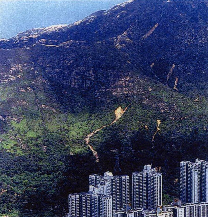
104                                                                    K. T. Chau and K. H. Lo: Hazard assessment of debris flows

Fig. 1. Debris flows that occurred on 14 April 2000 near Leung King Estate, which is in the foreground.

      Figure 1. Debris flows that occurred on April 14, 2000 near Leung King Estate, which is in
a large
      theamount  of factual, geological and simulated data, the
          foreground.                                                     The main objective of this study is to propose a method-
use of computer or information technology is crucial to the            ology for GIS-based hazard mapping that explicitly incor-
success of such analysis. Since the mid 1980s, geographical            porates the dynamics of debris flow. Leung King Estate is
information systems (GIS) have become a very popular tech-             selected for the present study as an example. A terrain model
nology for analyzing natural hazards, including landslides             of the Leung King area is first generated by using the Digi-
(Coppock, 1995). Some of these GIS-based hazard analy-                 tal Elevation Model (DEM) of the GIS-based digital contour
                                                                                                                       1
ses focus on earthquake-induced landslides (e.g. Luzi et al.,          map. Then, the topographical data from the terrain model is
2000), and some on rainfall-induced landslides (e.g. Miller            used in numerical simulations. The simulations use a flow
and Sias, 1998). GIS analysis has also been proposed to pro-           dynamics model modified from Takahashi et al. (1992). In
duce rockfall hazard maps (e.g. Cancelli and Crosta, 1994).            addition, a new erosion initiation criterion, which depends
However, the reliability of the hazard analysis does not de-           on the solid concentration in the flow, the percentage of fine
pend on which GIS software or platform is used but on what             solids, and the terminal settling velocity of particles in the
analysis method is employed (Carrara et al., 1999; Guzzetti            flow, proposed by Lo and Chau (2003) is also used. Poten-
et al., 2000). Therefore, various methods of analysis have             tial debris sources in Leung King area are identified, within
been proposed by many different authors (e.g. Carrara et al.,          which the potential volume of the largest debris flows along
1991; Dikau et al., 1996; Leroi, 1997; Guzzetti et al., 1999;          various gullies is estimated. The discharge histogram of the
Carrara et al., 1999; Guzetti et al., 2000; Dai and Lee, 2002a,        source based upon the flow rate measured by Pierson (1995)
b; Chau et al., 2003). One main limitation for all these anal-         for the debris flow induced by the 18 May 1980 eruption of
yses is that dynamics of debris flows or landslides has not            Mountain St. Helens is also assumed. The corresponding
been included in the hazard mapping.                                   solid concentrations in the histogram follow the data adopted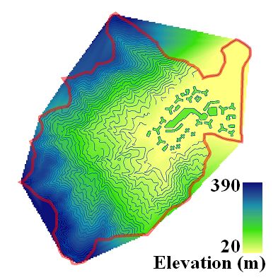
K. T. Chau and K. H. Lo: Hazard assessment of debris flows                                                                        105

in the simulation for the Horadani debris flow in Japan (pri-         2.1    The governing equations
vate communication, Takahashi and Nakagawa). Other de-
bris flow parameters are selected based on either suggestions         The flows of the fine and coarse particles through a small
by Takahashi et al. (1992) or interpreted data from the 1990          control volume satisfy the following continuity equations
Tsing Shan event, which occurred not too far from Leung               (Takahashi et al., 1992)
King Estate, as discussed by Lo and Chau (2003) and Lo
(2003). The results of the simulations predict the runout of          ∂ccp h ∂ccp M   ∂ccp N
                                                                            +       +        = iccp∗
future potential debris flows. A hazard map for Leung King             ∂t      ∂x       ∂y
Estate is generated using GIS based upon the results of the
numerical simulations. Finally, we also illustrate the genera-           (for coarse solid particles)                             (2)
tion of another hazard map of Leung King Estate by incorpo-
rating the results of numerical simulations and the statistical       ∂cfp h ∂cfp M   ∂cfp N
                                                                            +       +        = icfp∗
approach based on past landslide records.                               ∂t     ∂x       ∂y

                                                                              (for fine solid particles)                          (3)
2   Debris flow model
                                                                      where M and N are the average fluxes over flow depth h
In the literature, there is no theoretical flow model that can        along the x- and y-directions respectively. The velocity of
simulate debris flow over a three- dimensional terrain, that at       either gain or loss of the solid particles is denoted by i which
the same time takes into consideration changing of the bed by         is less than zero for deposition, and greater than zero for ero-
erosion and deposition. The only available models that can            sion. The subscript “∗ ” indicates either the solid concentra-
simulate three-dimensional debris flow approximately are the          tion of the eroded or the deposited debris mixtures at the
two-dimensional depth average models (e.g. Savage and Hut-            static bed. In this model, discharge histograms of both ccp
ter, 1991; Takahashi et al., 1992; O’Brien et al., 1993; Den-         and cfp must be input at an upstream boundary.
linger and Iverson, 2001; Ghilardi et al., 2001). Most of these          The momentum equations of the debris mixtures flowing
models did not incorporate erosion and deposition mecha-              along the x- and y-directions are respectively (Takahashi et
nism; only the models by Takahashi et al. (1992) and Ghi-             al., 1992):
lardi et al. (2001) incorporated the possibility of erosion and
                                                                      ∂M     ∂u0 M    ∂v0 M
deposition. In this study, we have adopted the model pro-                 +β       +β       =
posed by Takahashi et al. because it has been available for us         ∂t     ∂x       ∂y
to use (private communication, Takahashi and Nakagawa).
Without going into the details, we should emphasize a major                                           ∂(zb + h) τbx
                                                                            gh sin θbx − gh cos θbx            −    ,             (4)
limitation of the model by Takahashi et al. (1992), which is                                             ∂x      ρT
referred as the T-model hereafter. That is, the critical slope
gradient for the onset of erosion is assumed constant in the          ∂N    ∂u0 N    ∂v0 N
                                                                         +β       +β       =
model. This is only an approximation since the critical gradi-        ∂t     ∂x       ∂y
ent would naturally depend on the streampower of the flow.
Modification to the criterion for the onset of erosion will be                                        ∂(zb + h) τby
                                                                            gh sin θby − gh cos θby            −    ,             (5)
discussed in later section.                                                                              ∂y      ρT
   In the T-model, the mixture is assumed to consist of three
components, water, fine solid particles, and coarse solid par-        where g is the gravitational constant (9.81 m/s2 ); zb is the
ticles. The content of solids is represented by volumet-              deposit thickness; u0 and v0 are the velocities along x- and y-
ric concentrations of solid particles in the mixture (csp ), of       directions respectively; β is a momentum correction factor;
coarse solid particles in the mixture (ccp ), of fine solid parti-    ρT is the equivalent density of the debris mixture; θbx and
cles in mixture (cfp ), and of fine solid particles in interstitial   θby are the tangents at the bed along the x- and y-directions
fluid (cif ). They are defined as:                                    respectively; and τbx and τby are the base shear resistances
                                                                      along the x- and y-directions respectively. Full details of the
        Vs             Vc             Vf             Vf               T-model are referred to Takahashi et al. (1992) and Takahashi
csp =      ;   ccp =      ;   cfp =      ;   cif =      ,      (1)    (1981, 1991).
        VT             VT             VT             Vi

where Vf , Vc , Vi , and Vs are the volumes of fine solid par-        2.2 Modifications made to Takahashi’s model
ticles, coarse solid particles, interstitial fluid, and of total
solid particles respectively. Summing all Vf , Vc , and Vi            A new erosion initiation criterion has been proposed by Lo
equals the total volume of mixture VT ; and summing Vf                and Chau (2003). The full details of this modification are
and Vc equals Vs . Clearly, cif and cfp are not indepen-              beyond the scope of the present study. Only the main results
dent, and it is straightforward to show that they are related         will be summarized here. In particular, the minimum energy
by cfp =(1 − ccp )cif .                                               gradient, than θmin (i.e. a natural slope with energy gradient θ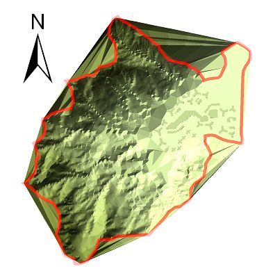
106 K. T. Chau and K. H. Lo: Hazard assessment of debris flows
a
b
○ Simulation
Field
Field
0 50 100 200 m
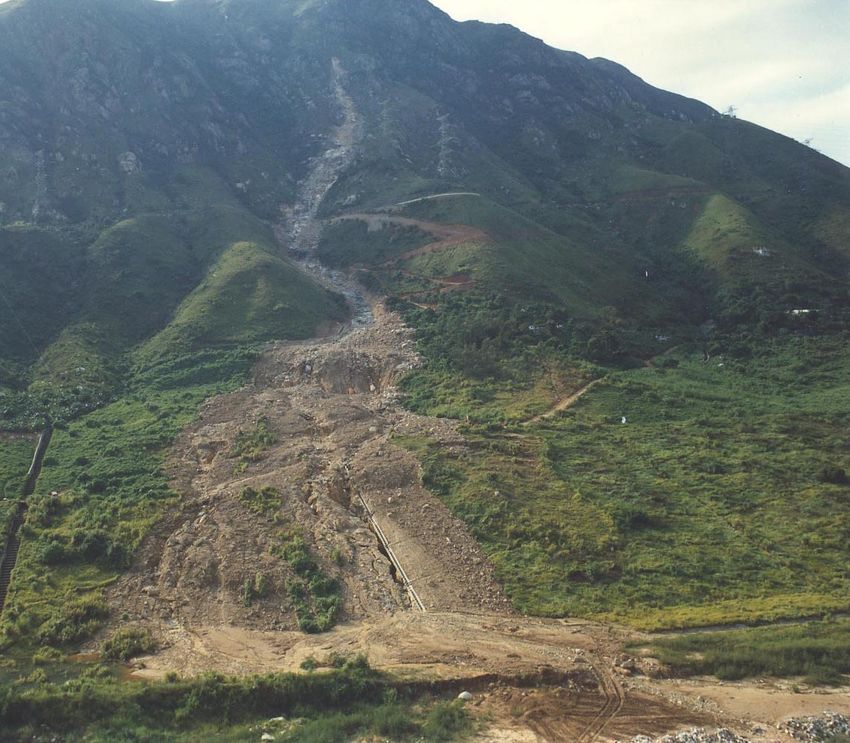
Fig. 2. (a) A photograph of the 1990 Tsing Shan debris flow; (b) Numerical simulation and field record. The shaded area labeled as “field”
in (b) is the field observation of the deposit area, whereas the open circles “o” denote the boundary of the deposit predicted in the numerical
simulation.
Figure 2. (a) A photograph of the 1990 Tsing Shan debris flow; (b) Numerical simulation and
field record.
less than The
θmin will shaded
suffer area
no erosion) labeled
is derived as2003;
as (Lo, “field”certain
in (b)particle
is thesizefield observation
d, average flow velocity ofalong
the the
deposit
x-
area, whereas
Lo and Chau , 2003):the open circles “o” denote the boundary of the deposit predicted
direction, average flow velocity along y-direction, densityinofthe
numerical simulation. the muddy water (i.e. the interstitial fluid), and relative set-
tan θmin =
R tling velocity of particle of size d respectively. The main con-
1
csp Gs ρw Pf ωr dP / 1 − Pf σ − 2ρ tribution from (6) is that the start of erosion is no longer set
m
tan sin−1 q (6) as an empirical constant, but a function of the fluid properties
2
Fρm u0 + v02 σ − ρ m
and flow energy. Thus, in general, θmin becomes a function
of the flow and thus changes with the position of the slope
where csp , F , Gs ,σ , ρw , Pf , P , u0 , v0 , ρm and ωr are
(as the flow parameters change along the slope profile). As
solid concentration in the flow, excess fraction of the stream-
shown by Lo (2003) and Lo and Chau (2003), after incorpo-
power available for erosion (typically 0.1–0.2), specific grav-
rating this erosion criterion, the simulations of the T-model
ity of the solid particles, density of the solid particles, den-
sity of water, percentage of fine solid (i.e. particle size less
fit better with the field record of the 1990 Tsing Shan debris 1
flow. The results are reported in the next section.
than 63 µm), percentage of solid mass in the fluid with a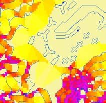
K. T. Chau and K. H. Lo: Hazard assessment of debris flows                                                                       107

                                                                    Leung King Estate
                    Study Area

                   ±

Fig. 3. The study area for debris flow hazard assessment of Leung King Estate.
      Figure 3. The study area for debris flow hazard assessment of Leung King Estate.

             (a)                                                           (b)
                                                                                                                          1
Fig. 4. (a) A contour map for generating the DEM of Leung King Estate; (b) the Digital Elevation Model (DEM) of Leung King Estate.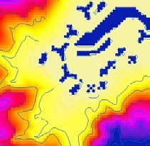
108                                                                K. T. Chau and K. H. Lo: Hazard assessment of debris flows

   If the channel slope θ along a gully is larger than the min-       Figure 2b shows the results of a particular simulation of
imun energy gradient θmin given by Eq. (6), the velocity of        the 1990 Tsing Shan debris flow by using the MT-model
erosion i defined in Eq. (2) can be determined from the fol-       summarized in the previous section. For the purpose of com-
lowing empirical formula (Takahashi et al., 1992):                 parison, the actual field observation is also reported Fig. 2a.
        p                                                          Figure 2 shows that the simulation result is comparable to
i = K gh sin3/2 θ                                                  that of the field observation, both in terms of the total deposit
                           1/2                               area as well as the runout displacement. The shaded area
       σ − ρi       tan α            tan α               h
  1−          ccp         −1               − 1 ccα − ccp    (7)    labeled as “field” in Fig. 2b is the field observation of the
         ρi         tan θ            tan θ                d
                                                                   deposit area, whereas the open circles denote the boundary
where K, g, σ , ρi , h, d, α and ccα are a numerical constant      of the deposit predicted in the numerical simulation. Based
(typically 0.06), the gravitational constant, the density of the   upon this comparison, the model parameters are calibrated
interstitial fluid, the density of the debris material, the flow   and are adopted for the simulations for Leung King Estate
depth, the mean diameter of solid particles, the dynamic fric-     area. In addition, we have also conducted a very comprehen-
tional angle, and the equilibrium solid concentration. Equa-       sive parametric study of the choice of various input parame-
tion (7) is obtained by assuming that erosion is caused by the     ters (Lo, 2003), but the details will not be given here.
dynamic action of the shear stress on the bed by the intersti-        We should emphasize here that the main objective of the
tial fluid of the overlying sediment-laden flow. This erosion      present study is not on the discussion of a particular debris
process is assumed to continue as long as the entrained-solids     flow simulation model (such as the MT-model), but instead
is less than the equilibrium value ccα . As shown in Eq. (7)       on the introduction of a methodology that incorporates nu-
that when ccp increases to ccα , the erosion velocity i dimin-     merical simulation for hazard mapping. Therefore, the de-
ishes to zero.                                                     tails of the numerical simulation are not crucial here. The full
                                                                   details are referred to Lo (2003). Indeed, the same methodol-
2.3   Parameter calibration using the 1990 Tsing Shan debris       ogy can also be applied for hazard mapping with other suit-
      flow                                                         able numerical simulation models, if it is deemed appropri-
                                                                   ate.
To illustrate the applicability of the present numerical model
(the modified Takahashi model or the MT model), the 1990
Tsing Shan debris flow occurred on the eastern flank of Ts-        3     Incorporation of numerical simulations with GIS
ing Shan is selected for parameter calibration. This event               mapping
occurred on 11 September 1990 and is the largest debris flow
in the recorded history of Hong Kong (see Fig. 2a). It was         In this section, we will demonstrate how to produce a “flow-
estimated that a total of 19 000 m3 of debris were deposited       dynamics-based” hazard map for Leung King Estate incor-
down slope. The total travel distance is about 1 km (King,         porating GIS technology. The selected area for our hazard
1996). Although this event is relatively well-documented,          study is shown in Fig. 3, and Leung King Estate is also indi-
similar to most other debris flows reported elsewhere no dis-      cated in the figure. The boundary of the study area coincides
charge histrograph was measured. Approximation becomes             with the catchment area for Leung King Estate.
inevitable in generating the histrographs for numerical sim-
                                                                   3.1     Generation of DEM for simulation
ulations. One simple way to establish the discharge histro-
graph is to assume that the general characteristics of dis-        In order to generate the topographical data required for the
charge are similar for different events. In particular, a de-      simulation using MT-model, a GIS-based digital map given
tailed literature review shows that most discharge histro-         in Fig. 4a is first converted to a Digital Elevation Model
graphs measured in field have an initial sharp increase in dis-    (DEM) (shown in Fig. 4b). The resolution of the DEM is
charge, followed by an exponential decay of the flow rate.         10 m × 10 m and is saved as raster in ArcGIS. This pixel or
One such example is the debris flow measured after the 1980        raster-based DEM for Leung King Estate is then converted
eruption of Mount. St. Helens (Pierson, 1995). Therefore,          to a data file format readable by the MT-model for the com-
in this study, the discharge histrograph recorded at Mount.        puter simulation. Each data point contains elevation and co-
St. Helens will be scaled down to match to the total vol-          ordinates, and this data set forms our topographical model.
ume of debris reported for the 1990 Tsing Shan debris flow.
Regarding the solid (both fine and coarse) concentrations in       3.2     Source identification and flow quantification
the discharge, we use the solid concentrations adopted for
the Horadani debris flow simulation (private communication,        3.2.1    Source zones
Takahashi and Nakagawa). Most of the other model parame-
ters can be estimated from the report of King (1996); if not,      Next step is to identify the potential source zones. After
they have been adopted from the data set for the Horadani de-      field trip work in the area and after studying the available
bris flow simulation. For example, the coarse and fine solid       aerial photographs, eight potential source zones were iden-
concentrations were obtained from the laboratory results re-       tified. They are labeled as (a) to (h) in Fig. 5. From field
ported by King (1996).                                             observation, the average thickness of colluvium in the source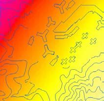
K. T. Chau and K. H. Lo: Hazard assessment of debris flows                                                                109

                ±
                                                                                (b)
                               (d)           (c)       (a)

                           (e)

                         (f)

                                                                                                 Leung King
                                                                                                   Estate

                                                                                               Mapped
                     (g)
                                                                                               Deposit

                                                             0            250   500                   1,000 m
                           (h)

   Fig. 5. Eight potential debris source zones, denoting by (a) to (h).

   areas is estimated from 1.3 m to 1.7 m. The total volume         3.2.3 Solid concentration histrograph
   of soil and boulders that may be mobilized from each zone
   can then be estimated from using a standard functions avail-     The ratio of coarse to fine solid concentrations are deter-
   able in ArcGIS. The accuracy of these estimated volumes          mined from laboratory data of soil sample from Tsing Shan,
Figure   5. Eight
   can always         potential
                be improved         debris
                              if more        source
                                      thorough          zones, denoting
                                                site investigations whereasbythe(a)  to (h). of solid concentrations are adopted
                                                                                 histrographs
   are conducted. These volumes form the basis for construct-       from those used for the Horadani debris flow simulation. The
   ing our inflow histrographs at the upstream boundary of each     solid concentration histrographs are given in Fig. 7 for all
   simulation.                                                      source areas (a) to (h). Again all plots are given in the same
                                                                    scale for easy comparisons. The amount of solid involved in
                                                                    each of these numerical simulations can be integrated from
   3.2.2 Discharge histrograph
                                                                    the discharge histrographs given in Fig. 6 in connection with
                                                                    the solid concentrations given in Fig. 7.
   In particular, after scaling the discharge histrograph of the                                                                 1
   debris flow of Mount. St. Helens, the histrograph for each       3.3 Results of numerical simulations
   source zone can be generated. They are given in Fig. 6 for all
   source zones (a) to (h). In order to put the magnitude of the    The results of the numerical simulations are given in Fig. 8
   discharge in the right perspective, all histrographs shown in    using ArcGIS. The deposition fan is marked by the dotted
   Fig. 6 are given on the same scale. As expected from Fig. 5,     lines, and the thickness of the deposition is indicated by
   the largest potential debris flow is likely to be from source    the darkness of the shaded areas within the marked areas
   area (h) followed by source area (f). The smallest discharge     of deposition. At some locations, the spatially distributed
   is from source area (e).                                         debris deposition can be up to 6 m thick (approximately
110 K. T. Chau and K. H. Lo: Hazard assessment of debris flows
25
0
25
×102m3/s)
Discharge (×
0
25
0
25
0
Time (sec.)
Fig. 6. Discharge histrographs for the source zones (a) to (h) shown in Fig. 5. The shapes of these histrographs are similar to that of the
debris flow occurred after the 1980 eruption of Mount St. Helens.
corresponding Figure
to the height of 2 storeys).
6. Discharge Exceptfor
histrographs forthe
simula- 3.4 (a)Debris
source zones to (h) flow
shownhazard map 5. The shapes
in Figure
tion from source area (e), all simulated debris flows reach the
of inside
buildings located these histrographs
Leung King are similar
Estate. Theto that of the debris
“Y”-shaped flowHazard
3.4.1 occurred after
map the solely
based 1980 eruption of simulation
on numerical
and “+”-shapedMount. St. Helens.
buildings are residential blocks within the
Estate while other facilities (like the shopping mall, primary By assuming the worst-case scenario that all debris flows oc-
and secondary schools) are denoted by polygons of different cur at the same time, we extract the maximum depth at each
shapes. Although the largest volume of debris is likely to be location from all eight numerical simulations shown in Fig. 8
from source zone (h), the most dangerous debris flow is the and the result is given in Fig. 9. The flow-dynamics-based
1
one from source zone (b) due to the proximity of the source plot provides a hazard map to identify the most dangerous
zone to downslope buildings and due to the steepness of the areas within the Estate. Based upon this map, remedial and
gully in which this debris flow would travel. The results of mitigation measures can be planned. The advantage of this
these simulations should, however, be interpreted with cau- kind of hazard map is that it is based purely on dynamics, in-
tion since they probably represent the worst scenarios related stead of on expert opinions or on past debris flow records.
to these source zones. In the case of heavy rain, one or more It is believed that it provides an improvement on the tra-
of these source zones may become fluidized and debris flow ditional way of generating GIS-based hazard maps, which
initiation may happen. However, it is very unlikely that all are based purely on statistical approach. It is because debris
potential debris flows will be mobilized at the same time, and flow hazard level at a particular location should depend on
the actual involved volume may also vary depending on the whether there is a chance of being affected by nearby po-
intensity of rain. tential sources instead of based purely on past records and
statistics.K. T. Chau and K. H. Lo: Hazard assessment of debris flows 111
0.5
0
0.5
Concentration
0
0.5
0
0.5
0
Time (sec.)
Fig. 7. Solid concentration histrographs for coarse, ccp , and fine, cfp , particles for the source zones (a) to (h) shown in Fig. 5. The ratio
of the fine to coarse solid concentration is set according to field measurements for Tsing Shan, whereas the shapes of histrographs are set
according to the Figure
Horadani7.debris
Solidflow
concentration
of Japan. histrographs for coarse, ccp, and fine, cfp, particles for the source
zones (a) to (h) shown in Figure 5. The ratio of the fine to coarse solid concentration is set
according
Of course, one to field
can always argue measurements for of
that the estimation Tsing
the Shan,
this whereas
figure, wethe
alsoshapes of histrographs
have labeled are set locations;
the most affected
total volume of mobilizable colluvium may not be accurate, they are a primary school (as P), a secondary school (as S),
according
and that the flow to the(MT-model
model itself Horadani indebris flow of
this case) may Japan.and two building blocks (as B1 and B2). It seems that debris
involve unwanted simplifications and assumptions. How- flow barriers should be installed in the future in protecting
ever, we can always conduct a more detailed site investiga- building blocks, S, B1, B2 and P. Although this plot is essen-
tion such that the extent and thickness of colluvium can be tially the same as Fig. 9, it provides a normalized basis for
estimated with higher certainty (if time and budget allow). combining the results of numerical simulations with other
Once a better or an improved theoretical model is available, factors affecting the hazard estimation.
the simulation can be conducted with higher accuracy. The
main focus here is not on the absolutely accuracy of the haz- 3.4.2 Hazard map combining numerical simulations 1 with
ard estimation, but on the idea of combining the sound the- other factors
oretical approach in GIS-base hazard mapping, such that ex-
pert opinion can be reduced to a minimum. If numerical simulations presented in the paper are not avail-
In addition, the results of our numerical simulations can able, the traditional way of assessing landslide hazard is to
also be normalized to give a hazard index map. For exam- correlate statistically the local geological features, including
ple, Fig. 10 gives a plot of the hazard index defined as the elevation, slope angle, and geology and environmental ef-
normalized thickness of the deposition (with respect to the fects to the actual landslide data. For example, in Fig. 11 the
maximum predicted thickness of the deposit in the area). In top four hazard index maps are given to indicate the effects112 K. T. Chau and K. H. Lo: Hazard assessment of debris flows
(a) (b)
±
(c) (d)
(e) (f)
(g) Deposition
(h)
0
0
0-2
0-2
2-4
2.000000001 - 4
4-6
4.000000001 - 6
6-8
6.000000001 - 8
8-10.5
8.000000001 - 10.5
0 50 100 200 m
Fig. 8. Results of the debris flow simulations for the source zones (a) to (h) shown in Fig. 5. Building footprints are given as unfilled
polygons. The legends in (h) for deposition thickness in metres.
Figure
of other factors,8. Results
such of the
as elevation, slopedebris flow and
angle, geology simulations forfour
For these thehazard
sourceindexzones
maps, we(a)refer
to to(h)
theshown
analy- in
rainfall. All these maps have been normalized with respect sis by Evans et al. (1999), who have examined the correla-
to theFigure
maximum 5.value
Building footprints
of the probability are given
of debris as unfilled
flow oc- polygons.
tions between natural The
terrainlegends
landslidein
(or(h) forflow)
debris deposition
oc-
currence within any class of each factor. currence and degree of erosion, terrain landform, lithology,
thickness are in meters.K. T. Chau and K. H. Lo: Hazard assessment of debris flows 113
± Potential Source Zone
Building
Deposit Depth (m)
0
0-2
2-4
4-6
6-8
8 - 10.5
Deposition Fan
Contour Line
0 50 100 200 m
Fig. 9. Combined result of the debris flow simulations of the source zones (a) to (h) shown in Fig. 8. Building footprints are given as unfilled
polygons. The legends in (h) for deposition thickness are in meters.
slope angle, slope aspect, elevation and vegetation for Hong rainfall maps published by the Hong Kong Observatory from
Kong using aerial photographs and GIS. For example, the ge- 1990 to 2000. In particular, the monthly rainfall maps with
Figure
ological 9. Combined
factor result
“elevation” can of the debris
be divided flow simulations
into 4 classes as: of the values
the maximum sourcewithin
zonesthe(a)
11 to (h)period
year shown from 1990 to
0–200 m, 200–400 m, 400–600 m and > 600 m (Evans et al., 2000 are extracted and averaged using raster calculator avail-
in Figure 8. Building footprints are given as unfilled polygons.
1999). Table 12 of Evans et al. (1999) shows that the densi- able in ArcGIS to yield the rainfall hazard raster map. Then,
ties of debris flow events per survey area (event/km) for these the map is normalized with respect to the maximum average
4 classes are 39.41, 40.06, 36.51, and 19.32 respectively. rainfall value to yield the hazard index map shown in Fig. 11.
Note that Evans et al. (1999) termed debris flow as natural The full details of the establishment of these hazard maps can
terrain landslides in their report. Consequently, normaliza- be referred to Chau et al. (2003).
tion gives the hazard index for the elevation hazard map with
index values of 0.9838, 1, 0.9114 and 0.4823 for the 4 differ- Once the hazard index maps with the maximum index
ent classses. Thus, an elevation-based hazard index map is value being unity are obtained for each factor (either geol-
generated with indices less than or equal to 1. Similarly, the ogy or environment), they can be combined to yield a fi-
data given in Tables 8 and 10 of Evans et al. (1999) can lead nal hazard map by assigning different weighting 1 to each
to the hazard index maps for geology and slope angle shown factor. For example, if hazard indices (H ji , i=1, 2, ..., n,
in Fig. 11. The rainfall hazard index maps are obtained from where n is the number of classes in each factor; j =1, 2..., m,
where m being the number of factors) with weightings114 K. T. Chau and K. H. Lo: Hazard assessment of debris flows
±
Hazard Index
0.00 - 0.45
0.45 - 0.50
S B2 0.50 - 0.55
0.55 - 0.60
B1 0.60 - 0.65
0.65 - 0.70
0.70 - 0.75
0.75 - 1.00
Building
Contour Line
P
0 50 100 200 m
Fig. 10. A hazard map based solely on computer simulations. The maximum index on the map is one. Building footprints are given as
unfilled polygons.
(Wj , j =1, 2, ..., m) are given, a hazard map can be gener- combining the top 4 hazard index maps for elevation, slope
ated. The number factors used in generating the hazard maps angle, geology and rainfall with corresponding weightings of
shown in Figs. 11a and b are m=4 and m=5 respectively. 1.0, 1.0, 0.5 and 1.0.
The landslide hazard at each location x (denoted by pixel of
However, if one incorporates the hazard index of numer-
10 m ×10 m) is calculated according to:
ical simulation given in Fig. 10 with a weighting of 1.0
Figure 10. AX m
hazard map X based
m
solely on computer simulations. Theformaximum
(which is selected index on
illustrative purpose the
only and in fact
Hazard(x)= [Wj Hj i (x)]/ Wj . (8) any weighting can be assigned) but assumes the total weight-
map is one. Building
j =1 footprints
j =1 are given as unfilled polygons.
ing in the denominator of (8) constant, Fig. 11b is obtained.
Since the values on the right hand side of (8) are scaled with Comparison of Figs. 11a and b reveals that the statistical haz-
respect to the sum of the weightings, the maximum value of ard map severely underestimates the potential debris flow
Hazard(x) at any pixel must be less than or equal to 1. The hazard at all building blocks S, P, B1 and B2 shown in
calculation of hazard map based upon Eq. (8) can be done Fig. 10. Thus, the traditional approach based purely on past
efficiently by using “raster calculator” available in ArcGIS. landslide record does not necessarily yield reliable results
Figure 11a shows a hazard map based purely on statistical compared to the flow-dynamics-based estimation. There-
analysis without using simulation results given in Fig. 10, by fore, it is unsafe to estimate hazard level based simply on a
1K. T. Chau and K. H. Lo: Hazard assessment of debris flows 115
Elevation Slope Angle Rainfall Geology
(a) (b)
± 0 50 100 200 m
Fig. 11. Four basic factor hazard maps for elevation, slope angle, rainfall and geology are shown in the top row. (a) A hazard map
combining the top four hazard maps (but without the results of numerical simulations); (b) A hazard map incorporating the results of
Figure
numerical 11. Four
simulations basic
given in Fig. 10factor hazard
(the weightings maps
for each forareelevation,
factor slope angle, rainfall and geology are
given in the text).
shown in the top row. (a) A hazard map combining the top four hazard maps (but without the
statistical approach, and numerical simulation results (which and Leung King Estate is selected as an example to illustrate
results of numerical simulations); (b) A hazard
estimating the travel distance of event from each potential how map incorporating
the debris flow hazard in the
term results of numerical
of deposition coverage
debris flow source zone) must be incorporated. and thickness can be generated. It is expected that the present
simulations given in Figure 10 (the weightingsmethodology for each factorwill be are given
further in totheother
applied text).
areas in Hong
Kong and other parts of the world. It is also demonstrated
4 Conclusions that it is unsafe and not conservative to estimate hazard level
based simply on a statistical approach, and numerical simula-
We have presented an approach to estimate the potential haz- tion results must be incorporated. This new approach opens
ard of debris flow by incorporating the results of numerical up a new direction for future research. In the long run, flow-
theoretical simulations of debris flow and GIS technol- dynamics-based GIS hazard mapping may better be received
ogy. The flow model adopted here is that of Takahashi et by city planners because of its sound theoretical background.
al. (1992), with appropriate modifications incorporated. The Nevertheless, much work remains to be done, before a robust
and efficient methodology can be applied for routine hazard
Tsing Shan debris flow of 1990 is used as a bench mark to
assessment.
1
calibrate the required parameters and data for simulations,116 K. T. Chau and K. H. Lo: Hazard assessment of debris flows
Acknowledgements. The work described in this paper was fully Ghilardi, P., Natale, L. and Savi, F.: Modeling Debris Flow Prop-
supported by the Research Grants Council of the Hong Kong agation and Deposition, Physics and Chemistry of the Earth,
Special Administrative Region, China and the Hong Kong Poly- 26(9), 651–656, 2001.
technic University (PolyU) through a research studentship to Guzzetti, F., Cardinali, M., Reichenbach, P., and Carrara, A.: Com-
KH Lo and through Projects A-PE79 and A 226. The authors paring landslide maps: A case study in the Upper Tiber River
are indebted to T. Takahashi and H. Nakagawa of Japan by basin, central Italy, Environmental Management, 25(3), 247–
generously providing the computer program for our work and 263, 2000.
providing useful references of their works. The support from Guzzetti, F., Carrara, A., Cardinali, M., and Reichenbach, P.: Land-
J. W. Z. Shi and Z. L. Li (of Department of Land Surveying slide hazard evulation: a review of current techniques and their
and Geo- informatics of PolyU) on the use of GIS technology application in a multi-scale study, Central Italy, Geomorphology,
and from Y. L. Sze on the use of the software ArcGIS is appreciated. 31(1-4), 181–216, 1999.
Halcrow China Limited: Investigation of some selected landslides
Edited by: P. Reichenbach in 2000, GEO Report No. 129, GEO, Civil Engineering Depart-
Reviewed by: D. Calcaterra and W. Savage ment, HKSAR, 2002.
Hansen, A.: Landslide hazard analysis, in: Slope Instability, Chap-
ter 13, edited by Brunsden, D. and Prior, D. B., Wiley, New York,
References 523–602, 1984.
Hungr, O.: Some methods of landslides hazard intensity mapping,
Cancelli, A. and Crosta, G.: Hazard and risk assessment in rock- in: Landslide Risk Assessment, edited by Cruden, D. M. and
fall prone areas, in: Risk and Reliability in Ground Engineering, Fell, R., Balkema, Rotterdam, 215–226, 1997.
edited by Skipp, B. O., Thomas Telford, 177–190, 1994. King, J. P.: The Tsing Shan debris flow, Special Project Report SPR
Carrara, A., Cardinali, M., Detti, R., Guzzetti, F., Pasqui, V., and 6/96, Hong Kong: Geotechnical Engineering Office, Civil Engi-
Reichenbach, P.: GIS techniques and statistical-models in evalu- neering Department, 1996.
ating landslide hazard, Earth Surface Processes and Landforms, Leroi, E.: Landslide risk mapping: Problems, limitation and devel-
16 (5), 427-445, 1991. opments, in: Landslide Risk Assessment, edited by Cruden, D.
Carrara, A., Guzzetti, F., Cardinali, M., and Reichenbach, P.: Use M. and Fell, R., Balkema, Rotterdam, 239–250, 1997.
of GIS technology in the prediction and monitoring of landslide Lo, K. H.: Numerical simulations of debris flow and their appli-
hazard, Natural Hazards, 20(2-3), 117–135, 1999. cation to hazard mapping using GIS, MPhil. Dissertation, De-
Chau K. T., Sze, Y. L., Fung, M. K., Wong, W. Y., Fong, E. L., partment of Civil and Structural Engineering, The Hong Kong
and Chan, L. C. P.: Landslide hazard analysis for Hong Kong Polytechnic University, Hong Kong, 2003.
using landslide inventory and GIS, Computers and Geosciences, Lo, K. H. and Chau, K. T.: Debris Flow Simulations for Tsing
in press, 2004. Shan in Hong Kong, Third International Conference on Debris-
Coppock, J. T.: GIS and natural hazards: An overview from a GIS Flow Hazards Mitigation: Mechanics, Prediction and Assess-
perspective, in: Geographical Information Systems in Assessing ment, September 10-12, 2003, Davos, Switzerland, vol. 1, 577–
Natural Hazards, edited by Carrara, A. and Guzzetti, F., Kluwer, 588, 2003.
Dordrecht, 21–34, 1995. Luzi, L., Pergalani, F., and Terlien, M. T. J.: Slope vulnerabil-
Dikau, R., Cavallin, A., and Jager, S.: Databases and GIS for land- ity to earthquakes at subregional scale, using probabilistic tech-
slide research in Europe, Geomorphology, 15(3-4), 227–239, niques and geographic information systems, Engineering Geol-
1996. ogy, 58(3-4), 313–336, 2000.
Dai, F. C. and Lee, C. F.: Landslide characteristics and, slope insta- Miller, D. J. and Sias, J.: Deciphering large landslides: linking hy-
bility modeling using GIS, Lantau Island, Hong Kong, Geomor- drological, groundwater and slope stability models through GIS,
phology, 42(3-4), 213–228, 2002a. Hydrological Processes, 12(6), 923–941, 1998.
Dai, F. C. and Lee, C. F.: Landslides on natural terrain – Physical O’Brien, J. P., Julien, P. J., and Fullerton, W. T.: Two-dimensional
characteristics and susceptibility mapping in Hong Kong, Moun- water flood and mudflow simulation, J. Hydr. Res., 119(2), 244–
tain Research and Development, 22(1), 40–47, 2002b. 261, 1993.
Denlinger, R. P. and Iverson, R. M.: Flow of variably fluidized Pierson, T.C.: Flow characteristics of large eruption-triggered de-
granular masses across three-dimensional terrain, 2. Numerical bris flows at snow-clad volcanoes: Constraints for debris-flow
predictions and experimental tests, J. Geophys. Res., 106(B1), models, J. Volcanol., 66, 283–294, 1995.
553–566, 2001. Savage, S. B. and Hutter, K.: The dynamics of avalanches of gran-
Einstein, H. H.: Landslide risk assessment procedure, in: Land- ular materials from initiation to runout, part I, Analysis, Acta
slides, 5th Int. Sym. on Landslides, Vol. 2, Balkema, Rotterdam, Mechanica, 86, 201–223, 1991.
1075–1090, 1988. Takahashi, T.: Debris flow, Annual Reviews Fluid Mechanics, 13,
Einstein, H. H.: Landslide risk-Systematic approaches to assess- 57–77, 1981.
ment, in: Landslide Risk Assessment, edited by Cruden, D. M. Takahashi, T.: Debris flow, International Association for Hydraulic
and Fell, R., Balkema, Rotterdam, 25–50, 1997. Research, Balkema, Rotterdam, 1991.
Evans, N. C., Huang, S. W., and King, J. P.: The natural terrain Takahashi, T., Nakagawa, H., Harada, T., and Yamashiki, Y.: Rout-
landslide study phases I and II, GEO Report No. 73, GEO, CED, ing debris flows with particle segregation, J. Hydr. Res., 118(11),
Hong Kong SAR Government, 128, 1999. 1490–1507, 1992.
Fell, R. and Hartford, D.: Landslide risk management, in: Landslide Varnes, D. J.: Landslide hazard zonation: A review of principles
Risk Assessment, edited by Cruden, D. M. and Fell, R., Balkema, and practice, UNESCO, France, 1–63, 1984.
Rotterdam, 51–109, 1997.You can also read