On Analysis of Seismic Vibrations Data Applying Doppler Effect Expression

Hindawi
Advances in Civil Engineering
Volume 2021, Article ID 8839828, 9 pages
https://doi.org/10.1155/2021/8839828

Research Article
On Analysis of Seismic Vibrations Data Applying Doppler
Effect Expression

 J. Skeivalas, E. K. Paršeli�
 unas, D. Šlikas , R. Obuchovski, and R. Birvydienė
 Institute of Geodesy, Vilnius Gediminas Technical University, Saulėtekis Av. 11, LT-10223 Vilnius, Lithuania

 Correspondence should be addressed to D. Šlikas; dominykas.slikas@vgtu.lt

 Received 28 September 2020; Revised 13 February 2021; Accepted 19 February 2021; Published 27 February 2021

 Academic Editor: Claudio Mazzotti

 Copyright © 2021 J. Skeivalas et al. This is an open access article distributed under the Creative Commons Attribution License,
 which permits unrestricted use, distribution, and reproduction in any medium, provided the original work is properly cited.

 In the paper, a possibility to develop the digital models of the seismic vibrations parameters is analyzed. To reach this goal, the
 observations at seismic station LUWI (Indonesia) were processed applying the statistical procedures. In fact, the biggest attention
 was given to the introduction of the Doppler effect expression and the employment of the theory of covariance functions. The
 trend in vectors of vibrations intensities values was detected and estimated upon using the least-squares method and polynomial
 approximation. In addition, by this technique, the random errors were eliminated partially. The self-developed computer
 programs based on Matlab programming package procedures were applied.

1. Introduction [31–34], GNSS [35–38], and satellite imagery [39–42].
 Several studies are dedicated to one of the most destructive
Earthquake is one of the most costly, devastating, and deadly eruptions—the 2018 Indonesia Sulawesi magnitude 7.5 Palu
natural hazards. Every disaster damages thousands of earthquake [34, 37, 41, 42].
buildings and displaces tens of thousands of people. The For Indonesia, from which the practical example in this
comprehensive knowledge of the earthquake nature and its paper is given, some research results could be found in
behavior is extremely important. Here the main task for [43–50]. Indonesia has a high seismicity rate, which is re-
scientists is to constrain the suitable mathematical methods lated to complex interaction of several tectonic plates
to analyse the earthquakes action, and most importantly to [51–63]. It should be especially noted that Indonesia’s
develop the earthquake model to predict its spread and to seismic region is an area of highest magnitude (more than
forecast its occurrence. The latest developments could be 6.0) eruptions [37, 60, 64–70].
noted in [1–7], where the biggest efforts were taken for What deals with scientific techniques and methods to
mathematical descriptions of wide earthquakes occurrence investigate earthquakes application has InSAR technology,
areas trying to construct the Ground Motion Prediction which enables detecting surface slips and Earth surface
Equations. Deep analysis of different aspects of passive deformations [34, 37, 41]. For example, the 4–7 m surface
seismic methods like a horizontal to vertical spectral ratio, slip in the area of Palu earthquake was detected [37] and the
which is often used to describe the earthquake site, could be maximum horizontal deformation was from 1.8 m till 3.6 m
found in [8–14]. Some characteristics of concrete earth- [41], when ALOS-2 interferogram showed a peak slip of
quake’s sites from world’s seismic zones are presented in 6.5 m located at the south of Palu city [34]. GNSS plays a
[9, 15–22]. In some papers, the stress was done on signif- great role in the research of earthquakes giving very precise
icance of three-dimensional modelling of seismic waves metrical parameters to improve the crustal deformation field
propagation [18, 23–27]. and 3D geometric complexities of the faults in total
 Various data sources were applied to investigate the [38, 53, 60, 65, 68]. Certainly, the main techniques to detect
phenomena of eruptions [28–30]. Great achievements are the technical parameters of earthquakes are seismograms
done using modern techniques like InSAR interferometry and the combinations of some techniques as well [34, 67]. So,

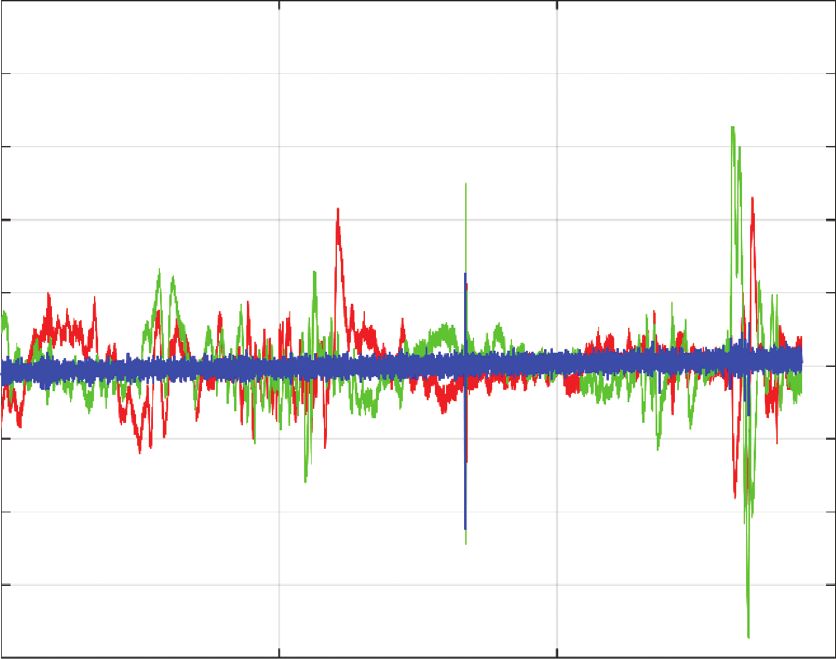
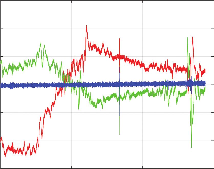
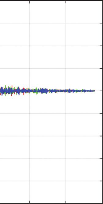
2 Advances in Civil Engineering

from broadband regional seismograms, it was revealed that ×105 Seismic parameters
the 2018 Palu earthquake is a supershear rupture event from 2
early on with an average rupture velocity of 4.1 km/s, and the 1.5
total seismic moment of 2.64 × 1020 Nm (equivalent to Mw

 Values of seismic parameters
 1
7.55) was released within 40 s [34].
 In this paper, we will show how the Doppler effect ex- 0.5
pression and the application of the theory of covariance 0
functions could be employed for seismic waves modelling. –0.5
The practical calculations were executed using the two
 –1
fragments of the observations data of the intensity φ of the
Earth’s seismic field, which were chosen from LUWI seismic –1.5
station (Sulawesi, Indonesia, latitude: −1.04180, longitude: –2
122.77170, elevation: 6.0 m): first on August 05, 2018, within
 –2.5
one hour (11:30–12:30), and second on November 11, 2018, 0 1 2 3 4 5 6 7
within two hours (5:00–7:00). At these periods, the seismic Epochs no. ×104
stations around the world have registered unusual vibrations
of low frequencies. Wide basic information on Palu earth- t21-BHE
quake could be found in specialized portals [71, 72]. t22-BHN
 t23-BHZ
 The observations data were expressed by vectors N
(North), E (East), and Z (Zenith). The time series views of the Figure 1: Time series of vectors N, E, and Z (LUWI station, August
centered vectors N, E, and Z for both abovementioned 05, 2018).
periods are presented in Figures 1 and 2. In both figures, the
time series views of the components E and N are similar. It
looks like the influence of the unusual low frequencies vi-
 Seismic parameters
brations in Figure 2 is possibly low. The systematic com- 3000
ponent of low frequency could be eliminated applying the 6-
degree polynomial approximation. It is presented in Fig- 2000
 Values of seismic parameters

ure 3. The accuracy of vectors N, E, and Z extracted from
LUWI station data on August 05, 2018, is described by 1000
standard deviations Sφ � (19480, 15926, 15810) cnt. These
numbers show that the accuracies of components of seismic 0
vectors presented in Figure 1 are approximately the same.
The accuracy of vectors N, E, and Z extracted from LUWI –1000
station on November 11, 2018 (if the systematic component
is not eliminated), is described by the vector of standard –2000
deviations Sφ � (1260, 559, 41) cnt. It shows that the accuracy
of observations is slightly higher at this period. The accuracy –3000
 0 5 10 15
of vectors N, E, and Z extracted on November 11, 2018 (if the
 Epochs no. ×104
systematic component is eliminated), is described by the
vector of standard deviations Sφ � (215, 257, 41) cnt. In this t1-BHE
case, the obtained accuracy of processed observation data is t2-BHN
considerably higher. t3-BHZ
 Mathematical-statistical methods are widely applied for Figure 2: Time series of vectors N, E, and Z (LUWI station,
data processing in geophysics, geodesy, and other Earth November 11, 2018).
sciences [73–75]. To predict and develop the model of the
spread of seismic vibrations, first of all, we assume that
seismic waves from the quake hypocenter spread as har- covariances of seismic field intensities vectors based on
monic vibrations of decreasing amplitudes in all the di- seismic observations data. The accuracies of corresponding
rections. So, we can assume also that the core structures of calculated parameters were obtained also.
seismic observations at the tracking stations mounted in The background of the mathematical model of obser-
short distances from the hypocenter and at those more vations data treatment is concept of a stationary random
distant are possibly very similar. For mathematical treatment function and especially paying attention to statement that
of the seismic observations, the covariance functions and the the errors of seismic vibrations observations are random
theory of Doppler effect were applied. The correlations and possibly are near the same precision. So we assume
between changes of intensities of seismic waves spreading in that the mathematical average of random errors
time and space were detected by introducing the variations MΔ � constant ⟶ 0, its dispersion DΔ � constant, and
of covariations of the seismic vibrations intensities vectors. the covariances of the observations depend on the difference
Some equations were derived to obtain the estimates of of the arguments only, so practically from the quantised
covariation matrixes and autocovariances and cross- intervals on the time scale.

Advances in Civil Engineering 3

 Seismic parameters where P is diagonal matrix (n × n) of weights pi of the values
 2500
 φi .
 2000 Weights pi could be detected according to simple
 Values of seismic parameters

 1500 formula:
 1000 σ 20
 pi � , (4)
 500 σ 2φi
 0
 where σ 0 is the standard deviation of the observation φ0 , the
 –500
 weight of which is supposed to be equal to unit, that is,
 –1000 p0 � 1.
 –1500 Furthermore, we can write the following equation:
 –2000 ui � ln φi , (5)
 0 5 10 15
 Epochs no. ×104 and we further obtain
 t1m-BHE σ φi � σ ui φi . (6)
 t2m-BHN
 t3-BHZ From formula (6), we can see that the value of σ φi
Figure 3: Time series of vectors N, E, and Z when the systematic pertains from the value of φi . So, the components, which
component is eliminated (LUWI station, November 11, 2018). have the bigger values, are of a lower accuracy just because
 φi ≫ σ ui .
 Upon applying formula (4), we write
2. Modelling of Seismic Vibrations
 σ 20 4
The observation data registered by the seismic station had pi � � 5 · φ−2
 i · 10 , (7)
 σ 2ui φi
been previously examined and processed upon reaching a
goal to eliminate both random and possibly systematic errors. where the accepted average value is σ 20 /σ 2ui � 5 · 104 .
 The most reliable values of the trend in the seismic vi- To find the extremum of function (3), let us calculate its
brations arrays were detected employing the least-squares . We can write and
 partial derivatives according to trend φ
method. Application of least-squares technique gives a solve the equation:
possibility to eliminate the random errors partially. While T
treating the big volumes of observations, the least-squares zΦ zε
 � 2 P · ε � 0. (8)
technique produces the asymptotically efficient values of the φ
 z φ
 z 
derived parameters also in case when a statistical distribu-
tion of the observations errors is not normal. Then we will obtain
 Any vector of seismic vibrations intensities could be −eT Pε � 0,
treated as a random function, which involves the random (9)
errors of observations. By employing a least-squares tech- eT Pe 
 φ − eT Pφ � 0.
nique to treat the vector of intensities φ, we can detect the
 of the trend. A parametric equation of a
most reliable value φ Thus, we will get the following solution:
single vector’s element φi will look like the following: −1
 � eT Pe eT Pφ � N− 1 ω,
 φ (10)
 ,
 εi � φi − φ (1)
 where N � (eT Pe), ω � eT Pφ.
where εi is a random error of the vector’s element, φi is the The accuracy of the trend could be detected by calcu-
 is vector’s trend.
value of the vector’s element, and φ lating its covariance matrix K φ :
 The expression in matrix form of equation (1) will be as K φ′ � σ ′2 ′2 − 1
 (11)
 φ � σ0 N ,
follows:
 ε � φ − e 
 φ, (2) where σ 0′ is the estimate of the standard deviation σ 0 . It is
 assessed by formula:
where ε is vector of random errors, φ � (φ1 , φ2 , . . . , φn )T is 1 T
vector of seismic field intensities, and e is vector of units σ ′2
 0 � ε Pε, (12)
 n−1
(n × 1).
 The most reliable value of vector φ trend could be cal- The considerably high systematic component of the
culated by introducing the general condition of the least- vibrations of the data of seismic station LUWI was elimi-
square method: nated upon applying a 6-degree polynomial approximation.
 Now, it is possible to calculate cross-covariance and
 Φ � εT Pε � min , (3) autocovariance functions of the seismic vibrations as well as

4 Advances in Civil Engineering

the shifts of the seismic vibrations, respectively, to each other The average magnitude Mzi of an argument z of the
by introducing the Doppler effect expression. Doppler formula could be expressed upon introducing the
 Let us take the formula for the parameter z [76–78]: vibrations intensities at the moment in time ti applying the
 fe f − fo following formula:
 z� −1� e , (13) 1
 fo fo Mzi � K ΔBei , Boi . (18)
 σ 2B
where fe is frequency of emitted vibrations and fo is fre-
quency of observed vibrations. By employing the theory of the covariance functions, it is
 We accept that the changes of vibrations phases ob- possible to express the cross-covariance functions of the
served at tracking stations possibly correspond to the corresponding seismic vibrations vectors taking into ac-
changes of the seismic vibrations intensities. Conse- count the fact that every vector of vibrations intensities
quently, sum of the seismic vibrations intensities is pro- could be treated as a random function as follows [77, 79, 80]:
portional to the algebraic sum of the frequencies phases of
vibrations accordingly; that is, K ΔBe , Bo � Kz (τ) � M δΔBe (u) · δBo (u + τ) ,
 T−τ (19)
 δB ∼ δω; (14) 1
 or Kz (τ) � δΔBe (u) · δBo (u + τ)du,
 T−τ 0
here δB, δω are changes of vibrations intensities and vi-
brations frequencies phases, respectively. where u is argument of any seismic vibrations vector, τ � s · Δ
 We can write the expressions for changes of vibrations is quantised interval, which is variable, s is number of quantised
intensities and the sum of them as follows: intervals, Δ is the value of the accepted unit of observations, and
 T is the diapason of the fluctuations of seismic vectors elements.
 δa(t) � Aδω · cos ωt, By using the vectors of observations data, an estimation
 δae (t) − δao (t) � Ae δωe · cos ωe t − A0 δωo · cos ωo t, Kz′(τ) of the cross-covariance function could be calculated
 according to the following formula:
 (15)
 1 n−s
where ωe � 2πfe , 2πfo , and the initial phases φ0 are sup- Kz′(τ) � Kz′(s) � δΔBe ui · δBo ui+s , (20)
 n − s i�1
posed to be equal to zero; δa ⟶ δB.
 By employing the parameter z of the Doppler effect where n is number of vector elements.
formula, we can express the strength of the seismic vibra- Now, using formula (18) in the vector form, we get the
tions at the moment in time ti : formula to detect the mathematical average of the argument
 δBei δB − δBoi z of the Doppler effect expression:
 zi � − 1 � ei , (16)
 δBoi δBoi Kz′(s) Kz′(s)
 Mz � � , (21)
where Bei is the intensity of emitted seismic vibrations, Boi is m.σ ′2
 B
 m.Kz′(0)
the intensity of observed seismic vibrations, Bei ∼ ωei , and
 where σ ′2 ′
 B ⟶ Kz(0) is the estimate of the dispersion and m
Boi ∼ ωoi .
 is number of cross-covariance values.
 In further developments, we employ the theory of co-
variance functions to detect the value of the argument z from
the Doppler effect expression. Mathematical derivations are 3. Analysis of the Experimental Results
grounded on the conception of a stationary random function
considering that errors of observations of seismic vibrations The estimates of autocovariance and cross-covariance
are random and possibly have similar precision. functions of the seismic vibrations intensities could be
 It is possible to express a cross-covariance function of the calculated employing formula (20). The values of the
straight algebraic sum ΔBei � Bei − Boi of the two intensities quantised intervals were assigned from 1 to n/2. Here,
Bei and Boi (emitted and observed) at a moment in time ti n � 144000 is the number of seismic vibrations vector
and a separate intensity Boi as follows: components. The graphical images of autocovariance and
 cross-covariance functions were generated also. Some
 K ΔBei � K δΔBei � M δΔBei · δBoi graphical images of covariance functions are shown in
 Figures 4–9.
 � M δBoi zi + 1 − δBoi · δBoi (17)
 2
 � M δ Boi · Mzi � σ 2B .Mzi , Upon applying formula (21), the mathematical averages
 of the argument z of the Doppler expression were detected.
where δBoi � Boi − MBoi , δBei � Bei − MBei , δBei � δBoi The positive values of the argument z point out that the
(zi + 1), MBoi , MBei are the average values of vibrations seismic vibrations recede from each other. The negative
intensities; δΔBoi � δBei − δBoi , σ B are the standard devia- values of the argument z indicate that seismic vibrations
tions of the vibrations intensities. It is supposed that the approach each other. The calculated approximate reciprocal
standard deviations of the observed and registered seismic velocity of seismic vibrations, registered in vectors N and E,
vibrations intensities are equal. is about v � 90 km/s.

Advances in Civil Engineering 5

 Function of correlations kfr2 Function of correlations kfr12
 1 0.5

 0.4
 0.8
 0.3

 Values of correlations ke
 Values of correlations ke

 0.6
 0.2

 0.4 0.1

 0
 0.2
 –0.1
 0
 –0.2

 –0.2 –0.3
 0 1 2 3 4 5 6 7 8 0 1 2 3 4 5 6 7 8
 Quantised intervals k ×104 Quantised intervals k ×104

Figure 4: Image of the normed autocovariance function of the Figure 7: Image of the normed cross-covariance function of the
vector N. two vectors N and E.

 Function of correlations kfr1 Function of correlations kfr13
 1 0.12

 0.8 0.1
 0.08
 Values of correlations ke
 Values of correlations ke

 0.6
 0.06
 0.4 0.04

 0.2 0.02
 0
 0
 –0.02
 –0.2
 –0.04
 –0.4 –0.06
 0 1 2 3 4 5 6 7 8 0 1 2 3 4 5 6 7 8
 Quantised intervals k ×104 Quantised intervals k ×104

Figure 5: Image of the normed autocovariance function of the Figure 8: Image of the normed cross-covariance function of the
vector E. two vectors E and Z.

 Function of correlations kfr3 Function of correlations kfr23
 1 0.08
 0.06
 0.8
 0.04
 Values of correlations ke
 Values of correlations ke

 0.6
 0.02
 0.4 0

 0.2 –0.02
 –0.04
 0
 –0.06
 –0.2
 –0.08
 –0.4 –0.1
 0 1 2 3 4 5 6 7 8 0 1 2 3 4 5 6 7 8
 Quantised intervals k ×104 Quantised intervals k ×104

Figure 6: Image of the normed autocovariance function of the Figure 9: Image of the normed cross-covariance function of the
vector Z. two vectors N and Z.

6 Advances in Civil Engineering

 Let us derive the estimates of the standard deviation of was suggested to detect the values of argument z
the argument z. It could be done in two ways. Firstly, z values from the Doppler effect formulas upon employing
could be detected upon applying the frequencies of vibra- the expression of the cross-covariance function of
tions emitted from earthquake source and observed fre- the sum of the intensities of seismic vectors com-
quencies of vibrations at seismic station. Secondly, z values ponents and the intensities of separate seismic vector
could be detected using the vibrations intensities. components.
 The formula to calculate the estimate of standard de- (2) For LUWI seismic station, the expressions of the
viation of the argument z using formula (13) could be written normed autocovariance functions of seismic vibra-
as follows: tions vectors N, E, and Z are slightly different. The
 σ 2fo σ 2fe f2e autocovariance of the components of seismic vector
 1 2 f2e 2
 σ 2z � σ fe + σ fo � ⎝
 ⎛ + ⎠ ⎞ Z has a maximum value of correlation r � 0.4. The
 f2o f4o f2o σ 2fo f2o (22) autocovariance of seismic vibrations vectors com-
 ponents is deep r ⟶ 1.0 at little values of quantised
 � 2 · 10− 16 1 +(z + 1)2 � 10 · 10− 16 , interval only, when k ⟶ 0(τ k ⟶ 0 s). The prob-
 abilistic dependence of the vector’s Z elements
 σ z′ � 3.0 · 10− 8 . (23) gradually decreases to r⟶0 at
 k ⟶ 50000(τ k ⟶ 2500 s). The autocovariance
 In formula (22), the estimate σ z′ of the standard deviation functions of the vectors N and E have the low var-
of the argument z was detected assuming σ fe � σ fo , z � 1.0, iable positive and negative values.
and σ fe /σ fo � 1.4 · 10− 8 . So, the ratio of the mathematical (3) The correlation values r of the normed cross-co-
average of the argument z is σ z′/z � 3.0 · 10− 8 . variance functions of components of vectors N, E,
 Let us derive the accuracy of the argument z of the and Z of tracking station are varying in a narrow
Doppler effect expression using the seismic vibrations in- range r ⟶ (−0.2: 0.4) along the whole quantised
tensities. Upon applying formulas (15), (16), and (22), we diapason. The values r of normed cross-covariance
have functions of components of vectors N, E, and Z are
 σ 2Bo σ 2ωo close to zero.
 σ 2zB � 2
 1 +(z + 1) � · 1 +(z + 1)2 , (4) The speed of reciprocal motion of seismic vector E
 B2o ω2o and N components was calculated. Its approximate
 (24)
 σω value v � 90 km/s.
 σ zB � 2.2 o � 2.2 · 1.4 · 10− 8 � 3 · 10− 8 ,
 ωo
 Data Availability
and the above was calculated upon considering
σ Be � σ Bo , σ fo /fo � σ ωo /ωo , and z � 1.0. The ratio of zB will be All data used during the research are available in a repository
σ zB′/zB � 3 · 10− 8 . online in accordance with funder data retention policies.
 The results of the calculations demonstrate that the Practically, data for this research were taken from the EIDA
detected accuracies of the argument z of the Doppler effect and GEOFON Data Archives (http://eida.gfz-potsdam.de/
expression are nearly the same in both cases: when registered webdc3/).
phases of vibrations frequencies or intensities (strengths) of
them are used in the calculation procedures. Disclosure
 Let us calculate the accuracy of the estimates of the The research was done as a part of employment at Vilnius
motion speed v � z · c. Upon using the equation Gediminas Technical University, Lithuania.
 ln v � ln z + ln c, (25)
 Conflicts of Interest
we can write the equation of the ratio as follows:
 The authors declare that there are no conflicts of interest.
 σ 2v σ 2z σ 2c
 � + , (26)
 v 2 z2 c 2 References
and (σ v /v) ≈ 3.0 · 10− 9 , when (σ c /c) � 3.0 · 10− 9 . [1] B.-J. Chiou and R. R. Youngs, “An NGA model for the average
 Introducing the above used data, we find that (σ v /v) � horizontal component of peak ground motion and response
3.0 · 10− 6 km/s, upon supposing that v � 1000 km/s. spectra,” Earthquake Spectra, vol. 24, no. 1, pp. 173–215, 2008.
 [2] B. S.-J. Chiou and R. R. Youngs, “Update of the chiou and
 youngs NGA model for the average horizontal component of
4. Conclusions peak ground motion and response spectra,” Earthquake
 Spectra, vol. 30, no. 3, pp. 1117–1153, 2014.
 (1) It was shown that employment of the Doppler effect [3] K. W. Campbell and Y. Bozorgnia, “NGA-West2 ground
 expression and the application of the theory of co- motion model for the average horizontal components of PGA,
 variance functions could be used to develop the PGV, and 5% damped linear acceleration response spectra,”
 digital models of the seismic vibrations. A method Earthquake Spectra, vol. 30, no. 3, pp. 1087–1115, 2014.

Advances in Civil Engineering 7

 [4] M. A. Marafi, M. O. Eberhard, and J. W. Berman, “Effects of [19] A. Berbellini, A. Morelli, and A. M. G. Ferreira, “Ellipticity of
 the yufutsu basin on structural response during subduction Rayleigh waves in basin and hard-rock sites in Northern
 earthquakes,” in Proceedings of the Sixteenth World Confer- Italy,” Geophysical Journal International, vol. 11, no. 2,
 ence on Earthquake Engineering, Santiago, Chili, January 2017. pp. 115–129, 2016.
 [5] N. A. Abrahamson, W. J. Silva, and R. Kamai, “Summary of [20] A. Berbellini, A. Morelli, and A. M. G. Ferreira, “Crustal
 the ASK14 ground motion relation for active crustal regions,” structure of northern Italy from the ellipticity of Rayleigh
 Earthquake Spectra, vol. 30, no. 3, pp. 1025–1055, 2014. waves,” Physics of the Earth and Planetary Interiors, vol. 265,
 [6] N. Abrahamson, N. Gregor, and K. Addo, “BC hydro ground pp. 1–14, 2017.
 motion prediction equations for subduction earthquakes,” [21] V. C. Tsai, D. C. Bowden, and H. Kanamori, “Explaining
 Earthquake Spectra, vol. 32, no. 1, pp. 23–44, 2016. extreme ground motion in Osaka basin during the 2011
 [7] B. Pandey, R. S. Jakka, A. Kumar, and H. Mittal, “Site Tohoku earthquake,” Geophysical Research Letters, vol. 44,
 characterization of strong-motion recording stations of Delhi no. 14, pp. 7239–7244, 2017.
 using joint inversion of phase velocity dispersion and H/V [22] K. Chimoto, H. Yamanaka, S. Tsuno, H. Miyake, and
 curve,” Bulletin of the Seismological Society of America, N. Yamada, “Estimation of shallow S-wave velocity structure
 vol. 106, no. 3, pp. 1254–1266, 2016. using microtremor array exploration at temporary strong
 [8] G. Tarabusi and R. Caputo, “The use of HVSR measurements motion observation stations for aftershocks of the 2016
 for investigating buried tectonic structures: the Mirandola Kumamoto earthquake,” Earth, Planets and Space, vol. 68,
 anticline, Northern Italy, as a case study,” International no. 1, p. 206, 2016.
 Journal of Earth Sciences, vol. 106, no. 1, pp. 341–353, 2016. [23] S. Castellaro, L. A. Padrón, and F. Mulargia, “The different
 [9] J. F. Borges, H. G. Silva, R. J. G. Torres et al., “Inversion of response of apparently identical structures: a far-field lesson
 ambient seismic noise HVSR to evaluate velocity and struc- from the Mirandola 20th May 2012 earthquake,” Bulletin of
 tural models of the Lower Tagus Basin, Portugal,” Journal of Earthquake Engineering, vol. 12, no. 5, pp. 2481–2493, 2014.
 Seismology, vol. 20, no. 3, pp. 875–887, 2016. [24] M. A. Denolle, E. M. Dunham, G. A. Prieto, and G. C. Beroza,
[10] U. N. Prabowo, Marjiyono, and Sismanto, “Mapping the “Strong ground motion prediction using virtual earthquakes,”
 fissure potential zones based on microtremor measurement in Science, vol. 343, no. 6169, pp. 399–403, 2014.
 Denpasar City, Bali,” IOP Conference Series: Earth and En- [25] L. Viens, H. Miyake, and K. Koketsu, “Long-period ground
 vironmental Science, vol. 29, Article ID 012012, 2016. motion simulation of a subduction earthquake using the
[11] E. Fergany and K. Omar, “Liquefaction potential of Nile delta, offshore-onshore ambient seismic field,” Geophysical Research
 Letters, vol. 42, no. 13, pp. 5282–5289, 2015.
 Egypt,” NRIAG Journal of Astronomy and Geophysics, vol. 6,
 [26] L. Viens, H. Miyake, and K. Koketsu, “Simulations of long-
 no. 1, pp. 60–67, 2017.
 period ground motions from a large earthquake using finite
[12] A. P. Singh, A. Shukla, M. R. Kumar, and M. G. Thakkar,
 rupture modeling and the ambient seismic field,” Journal of
 “Characterizing surface geology, liquefaction potential, and
 Geophysical Research: Solid Earth, vol. 121, no. 12,
 maximum intensity in the kachchh seismic zone, western
 pp. 8774–8791, 2016.
 India through microtremor analysis,” Bulletin of the Seis-
 [27] L. Viens, M. Denolle, H. Miyake, S. I. Sakai, and S. Nakagawa,
 mological Society of America, vol. 107, no. 3, 2017.
 “Retrieving impulse response function amplitudes from the
[13] V. Pazzi, L. Tanteri, G. Bicocchi, M. D’Ambrosio, A. Caselli,
 ambient seismic field,” Geophysical Journal International,
 and R. Fanti, “H/V measurements as an effective tool for the
 vol. 210, no. 1, pp. 210–222, 2017.
 reliable detection of landslide slip surfaces: case studies of [28] F. Løvholt, H. Hasan, S. Lorito et al., “Multiple source sen-
 Castagnola (La Spezia, Italy) and Roccalbegna (Grosseto, sitivity study to model the 28 September Sulawesi tsuna-
 Italy),” Physics and Chemistry of the Earth, Parts A/B/C, mi—landslide and strike slip sources,” in Proceedings of the
 vol. 98, pp. 136–153, 2017. AGU Fall Meeting 2018, Washington, DC, USA, December
[14] N. A. Zeid, E. Corradini, S. Bignardi, V. Nizzo, and 2018.
 G. Santarato, “The passive seismic technique “HVSR” as a [29] A. Van Dongeren, D. Vatvani, and M. van Ormondt, “Sim-
 reconnaissance tool for mapping paleo-soils: the case of the ulation of 2018 tsunami along the coastal areas in the Palu
 pilastri archaeological site, northern Italy,” Archaeological bay,” in Proceedings of the AGU Fall Meeting 2018, Wash-
 Prospection, vol. 24, no. 3, pp. 245–258, 2017. ington, DC, USA, December 2018.
[15] M. V. Manakou, D. G. Raptakis, F. J. Chávez-Garcı́a, [30] R. Omira, G. G. Dogan, R. Hidayat et al., “The September
 P. I. Apostolidis, and K. D. Pitilakis, “3D soil structure of the 28th, 2018, tsunami in Palu-Sulawesi, Indonesia: a post-event
 Mygdonian basin for site response analysis,” Soil Dynamics field survey,” Pure and Applied Geophysics, vol. 176, no. 4,
 and Earthquake Engineering, vol. 30, no. 11, pp. 1198–1211, pp. 1379–1395, 2019.
 2010. [31] A. Hooper, D. Bekaert, K. Spaans, and M. Arıkan, “Recent
[16] M. Pilz, S. Parolai, M. Stupazzini, R. Paolucci, and J. Zschau, advances in SAR interferometry time series analysis for
 “Modelling basin effects on earthquake ground motion in the measuring crustal deformation,” Tectonophysics, vol. 514–517,
 Santiago de Chile basin by a spectral element code,” Geo- pp. 1–13, 2012.
 physical Journal International, vol. 187, no. 2, pp. 929–945, [32] M. Lesko, J. Papco, M. Bakon, and P. Liscak, “Monitoring of
 2011. natural hazards in Slovakia by using of satellite radar inter-
[17] A. Iwaki and T. Iwata, “Estimation of three-dimensional ferometry,” Procedia Computer Science, vol. 138, pp. 374–381,
 boundary shape of the Osaka sedimentary basin by waveform 2018.
 inversion,” Geophysical Journal International, vol. 186, no. 3, [33] A. M. Lubis, T. Sato, N. Tomiyama, N. Isezaki, and
 pp. 1255–1278, 2011. T. Yamanokuchi, “Ground subsidence in Semarang-Indo-
[18] V. M. Cruz-Atienza, J. Tago, J. D. Sanabria-Gomez et al., nesia investigated by ALOS-PALSAR satellite SAR interfer-
 “Long duration of ground motion in the paradigmatic valley ometry,” Journal of Asian Earth Sciences, vol. 40, no. 5,
 of Mexico,” Nature, vol. 6, no. 38807, 2016. pp. 1079–1088, 2011.

8 Advances in Civil Engineering

[34] J. Fang, C. Xu, Y. Wen et al., “The 2018 Mw 7.5 Palu [49] A. Koulali, S. McClusky, S. Susilo et al., “The kinematics of
 earthquake: a supershear rupture event constrained by InSAR crustal deformation in Java from GPS observations: impli-
 and broadband regional seismograms,” Remote Sensing, cations for fault slip partitioning,” Earth and Planetary Science
 vol. 11, no. 11, p. 1330, 2019. Letters, vol. 458, pp. 69–79, 2017.
[35] A. Walpersdorf, C. Rangin, and C. Vigny, “GPS compared to [50] A. M. Pramatadie, H. Yamanaka, K. Chimoto et al.,
 long-term geologic motion of the north arm of Sulawesi,” “Microtremor exploration for shallow S-wave velocity
 Earth and Planetary Science Letters, vol. 159, no. 1-2, structure in Bandung basin, Indonesia,” Exploration Geo-
 pp. 47–55, 1998a. physics, vol. 48, no. 4, pp. 401–412, 2016.
[36] A. Walpersdorf, C. Vigny, C. Subarya, and P. Manurung, [51] J. A. Katili, “Large transcurrent faults in Southeast Asia with
 “Monitoring of the Palu-Koro fault (Sulawesi) by GPS,” special reference to Indonesia,” Geologische Rundschau,
 Geophysical Research Letters, vol. 25, no. 13, pp. 2313–2316, vol. 59, no. 2, pp. 581–600, 1970.
 1998b. [52] N. Hurukawa, B. R. Wulandari, and M. Kasahara, “Earth-
[37] A. Socquet, J. Hollingsworth, E. Pathier, and M. Bouchon, quake history of the Sumatran fault, Indonesia, since 1892,
 “Evidence of supershear during the 2018 magnitude 7.5 Palu derived from relocation of large earthquakes,” Bulletin of the
 earthquake from space geodesy,” Nature Geoscience, vol. 12, Seismological Society of America, vol. 104, no. 4, pp. 1750–
 no. 3, pp. 192–199, 2019. 1762, 2014.
[38] T. Tabei, F. Kimata, T. Ito et al., “Geodetic and geomorphic [53] A. Julzarika and C. A. Rokhmana, “Detection of vertical
 evaluations of earthquake generation potential of the deformation in Jakarta-Bandung high speed train route using
 Northern Sumatran Fault, Indonesia,” in Proceedings of the X sar and sentinel,” Geodesy and Cartography, vol. 45, no. 4,
 International Association of Geodesy Symposia, International pp. 169–176, 2019.
 Symposium on Geodesy for Earthquake and Natural Hazards [54] D. H. Natawidjaja, “Updating active fault maps and sliprates
 (GENAH), Kyoto, Japan, June 2015. along the Sumatran Fault Zone, Indonesia,” IOP Conference
[39] M. De Michele, “Subpixel offsets of copernicus sentinel 2 data, Series: Earth and Environmental Science, vol. 118, no. 1, Article
 related to the displacement field of the Sulawesi earthquake ID 012001, 2018.
 (2018, Mw 7.5),” 2019. [55] O. Bellier, M. Sébrier, T. Beaudouin et al., “High slip rate for a
[40] S. Valkaniotis, A. Ganas, V. Tsironi, and A. Barberopoulou, “A low seismicity along the Palu-Koro active fault in central
 preliminary report on the M7.5 Palu 2018 earthquake co- Sulawesi (Indonesia),” Terra Nova, vol. 13, no. 6, pp. 463–470,
 2001.
 seismic ruptures and landslides using image correlation
 [56] O. Bellier, M. Sébrier, D. Seward, T. Beaudouin,
 techniques on optical satellite data,” 2018.
 M. Villeneuve, and E. Putranto, “Fission track and fault ki-
[41] Y. Wang, W. Feng, K. Chen, and S. Samsonov, “Source
 nematics analyses for new insight into the Late Cenozoic
 characteristics of the 28 september 2018 Mw 7.4 Palu, Indo-
 tectonic regime changes in West-Central Sulawesi (Indo-
 nesia, earthquake derived from the advanced land observation
 nesia),” Tectonophysics, vol. 413, no. 3-4, pp. 201–220, 2006.
 satellite 2 data,” Remote Sensing, vol. 11, no. 17, p. 1999, 2019.
 [57] M. R. Daryono, “Paleoseismologi tropis Indonesia (dengan
[42] M. Syifa, P. Kadavi, and C.-W. Lee, “An artificial intelligence
 studi kasus di sesar sumatra, sesar palukoro-matano, dan sesar
 application for post-earthquake damage mapping in palu,
 lembang),” 2018.
 central Sulawesi, Indonesia,” Sensors, vol. 19, no. 3, p. 542,
 [58] O. Heidbach, M. Rajabi, X. Cui et al., “The World stress map
 2019. database release 2016: crustal stress pattern across scales,”
[43] E. Saygin, P. R. Cummins, A. Cipta et al., “Imaging archi- Tectonophysics, vol. 744, pp. 484–498, 2018.
 tecture of the Jakarta Basin, Indonesia with transdimensional [59] E. Pelinovsky, D. Yuliadi, G. Prasetya, and R. Hidayat, “The
 inversion of seismic noise,” Geophysical Journal International, 1996 Sulawesi tsunami,” Natural Hazards, vol. 16, no. 1,
 vol. 204, no. 2, pp. 918–931, 2016. pp. 29–38, 1997.
[44] E. Saygin, P. R. Cummins, and D. Lumley, “Retrieval of the P [60] A. Socquet, W. Simons, C. Vigny et al., “Microblock rotations
 wave reflectivity response from autocorrelation of seismic and fault coupling in SE Asia triple junction (Sulawesi,
 noise: Jakarta Basin, Indonesia,” Geophysical Research Letters, Indonesia) from GPS and earthquake slip vector data,”
 vol. 44, no. 2, pp. 792–799, 2017. Journal of Geophysical Research, vol. 111, no. B8, Article ID
[45] M. Ridwan, S. Widiyantoro, M. Irsyam, Afnimar, and B08409, 2006.
 H. Yamanaka, “Development of engineering bedrock map [61] Y. Tanioka, Yudhicara, T. Kususose et al., “Rupture process of
 beneath Jakarta based on microtremor array measurements,” the 2004 great Sumatra-Andaman earthquake estimated from
 Geological Society, London, Special Publications, vol. 441, tsunami waveforms,” Earth, Planets and Space, vol. 58, no. 2,
 no. 1, pp. 153–165, 2016. pp. 203–209, 2006.
[46] A. Cipta, R. Robiana, J. Griffin, N. Horspool, S. Hidayati, and [62] A. Cipta, R. Robiana, J. D. Griffin, N. Horspool, S. Hidayati,
 P. Cummins, “A probabilistic seismic hazard assessment for and P. R. Cummins, “A probabilistic seismic hazard assess-
 Sulawesi, Indonesia,” in Geohazards in Indonesia: Earth ment for Sulawesi, Indonesia,” Geological Society, London,
 Science for Disaster Risk Reduction Geol. Soc., London, Special Special Publications, vol. 441, no. 1, pp. 133–152, 2017.
 Publications 441, P. R. Cummins and I. Meilano, Eds., The [63] I. M. Watkinson and R. Hall, “Fault systems of the eastern
 Geological Society of London, London, UK, 2016. Indonesian triple junction: evaluation of Quaternary activity
[47] A. Cipta, P. Cummins, M. Irsyam, and S. Hidayati, “Basin and implications for seismic hazards,” Geological Society,
 resonance and seismic hazard in jakarta, Indonesia,” Geo- London, Special Publications, vol. 441, no. 1, pp. 71–120, 2017.
 sciences, vol. 8, no. 4, p. 128, 2018. [64] R. Zuo, C. Qu, X. Shan, G. Zhang, and X. Song, “Coseismic
[48] L. Handayani, M. Maryati, K. Kamtono, M. Mukti, and deformation fields and a fault slip model for the Mw7.8
 Y. Sudrajat, “Audio-magnetotelluric modeling of cimandiri mainshock and Mw7.3 aftershock of the Gorkha-Nepal 2015
 fault zone at Cibeber, Cianjur,” Indonesian Journal on Geo- earthquake derived from Sentinel-1A SAR interferometry,”
 science, vol. 4, pp. 39–47, 2017. Tectonophysics, vol. 686, pp. 158–169, 2016.

Advances in Civil Engineering 9

[65] X. Song, Y. Zhang, X. Shan, Y. Liu, W. Gong, and C. Qu,
 “Geodetic observations of the 2018 Mw 7.5 Sulawesi earth-
 quake and its implications for the kinematics of the Palu
 fault,” Geophysical Research Letters, vol. 46, no. 8,
 pp. 4212–4220, 2019.
[66] H. Bao, J.-P. Ampuero, L. Meng et al., “Early and persistent
 supershear rupture of the 2018 magnitude 7.5 Palu earth-
 quake,” Nature Geoscience, vol. 12, no. 3, pp. 200–205, 2019.
[67] Y. Zhang, Y.-T. Chen, and W. Feng, “Complex multiple-
 segment ruptures of the 28 September 2018, Sulawesi,
 Indonesia, earthquake,” Science Bulletin, vol. 64, no. 10,
 pp. 650–652, 2019.
[68] T. Ulrich, S. Vater, E. H. Madden et al., “Coupled, physics-
 based modeling reveals earthquake displacements are critical
 to the 2018 3 Palu, Sulawesi Tsunami,” 2019.
[69] P. L. F. Liu, I. Barranco, H. M. Fritz et al., “What we do and
 don’t know about the 2018 Palu Tsunami—a future plan,” in
 Proceedings of the AGU Fall Meeting 2018, Washington, DC,
 USA, December 2018.
[70] M. Carvajal, C. Araya-Cornejo, I. Sepúlveda, D. Melnick, and
 J. S. Haase, “Nearly instantaneous tsunamis following the Mw
 7.5 2018 palu earthquake,” Geophysical Research Letters,
 vol. 46, no. 10, p. 5117, 2019.
[71] US Geological Survey, Mw 7.5 Palu earthquake, Indonesia, US
 Geological Survey, Reston, VA, USA, 2018, https://
 earthquake.usgs.gov/earthquakes/eventpage/us1000h3p4/
 executive#executive.
[72] Geoscope Observatory, Mw 7.5 Earthquake, Sulawesi 2018/09/
 28 10:02:43 UTC, http://geoscope.ipgp.fr/index.php/en/
 catalog/earthquake-description?seis=us1000h3p4, 2018.
[73] A. Sas-Uhrynowski, H. Karatayev, S. Mroczek, and
 O. Karagodina, “Research of the secular variation of the
 geomagnetic field on Polish and Belarus territory,” Prace
 IGiK, Tom XLVII, vol. 100, pp. 25–34, 2000.
[74] J. Marianiuk and J. Reda, Results of Geomagnetic Observations,
 Publications of the Institute of geophysics, Polish Academy of
 Science, C-79 (328), Belsk, Poland, 2001.
[75] A. Czyszek and J. Czyszek, Results of Geomagnetic Observa-
 tions, Hel, 2000, Publications of the Institute of geophysics,
 Polish Academy of Science, Warszawa, Poland, 2002.
[76] H. Kahmen, Elektronische Messverfahren in der Geodäsie.
 Grundlagen und Anwendungen, Verlag Karsruhe, Gliwice,
 Poland, 1978.
[77] J. Skeivalas, E. K. Paršeli�
 unas, D. Šlikas et al., “Predictive
 models for identification of parameters of seismic vibrations
 by applying the theory of covariance functions,” Indian
 Journal of Physics, vol. 95, 2019.
[78] J. Skeivalas, V. Turla, and M. Jurevicius, “Predictive models of
 the galaxies’ movement speeds and accelerations of move-
 ment on applying the Doppler effect,” Indian Journal of
 Physics, vol. 93, no. 1, pp. 1–6, 2019b.
[79] K. R. Koch, Einführung in die Byes-Statistik, Springer-Verlag
 Berlin Heidelberg, Berlin, Germany, 2000.
[80] J. Skeivalas and E. Parseliunas, “On identification of human
 eye retinas by the covariance analysis of their digital images,”
 Optical Engineering, vol. 52, no. 7, Article ID 073106, 2013.