Unsupervised topological learning for atomic structures identification
←
→
Page content transcription
If your browser does not render page correctly, please read the page content below
Unsupervised topological learning
                                                                          for atomic structures identification

                                                             Sébastien Becker1,2 , Emilie Devijver2 , Rémi Molinier3 , and Noël Jakse1
                                                                                       1
                                                                                           Univ. Grenoble Alpes,
                                                                                   CNRS, Grenoble INP, SIMaP,
arXiv:2109.08126v1 [cond-mat.dis-nn] 16 Sep 2021

                                                                                      F-38000 Grenoble, France
                                                                                       2
                                                                                           Univ. Grenoble Alpes,
                                                                                    CNRS, Grenoble INP, LIG,
                                                                                      F-38000 Grenoble, France
                                                                                       3
                                                                                           Univ. Grenoble Alpes,
                                                                                CNRS, IF, F-38000 Grenoble,France

                                                                                     (Dated: September 17, 2021)

                                                                                                 Abstract
                                                     We propose an unsupervised learning methodology build on a Gaussian mixture model computed
                                                   on topological descriptors from persistent homology, for the structural analysis of materials at
                                                   the atomic scale. Based only on atomic positions and without a priori knowledge, our method
                                                   automatically identifies relevant local atomic structures in a system of interest. Along with a
                                                   complete description of the procedure, we provide a concrete example of application by analysing
                                                   large-scale molecular dynamics simulations of bulks crystal and liquid as well as homogeneous
                                                   nucleation events of elemental Zr at the nose of the time-temperature-transformation curve. This
                                                   method opens the way to deeper and autonomous studies of structural dependent phenomena
                                                   occurring at the atomic scale in materials.

                                                                                                   1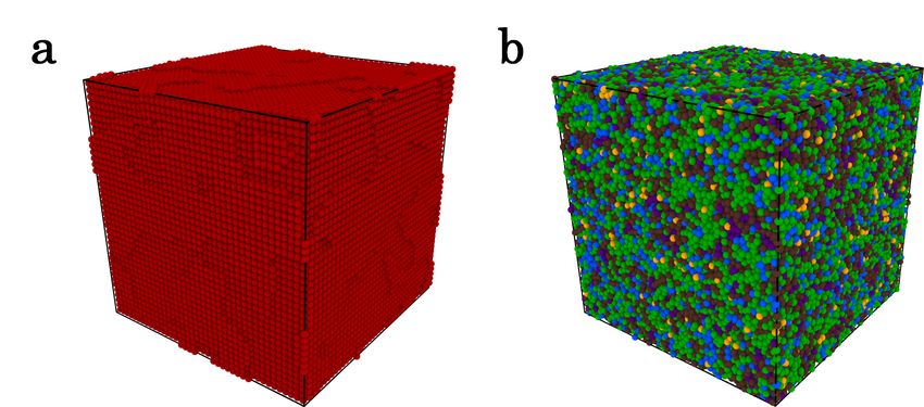
I.    INTRODUCTION

     Knowledge of microscopic events which drive macroscopic properties is of a fundamental
interests in the description of materials. The understanding of structural phenomena at the
atomic scale is indeed of a crucial role in the potential conception of new materials, which
can be part of the resolution of contemporary societal issues such as the reduction of energy
consumption or even conception of new drugs [1]. However, lot of information at such low
spatial scale of the order of the ångström is still out of reach experimentally.
     To access to physical and chemical properties at the atomic scale, molecular dynamics
(MD) stands as a powerful simulation tool [2]. With the growing computational capacity
at disposal, such simulations can nowadays easily reach millions of atoms evolving through
several nanoseconds. However, although this production of a lot of valuable data have been
streamlined, the processing of this so called “big data” have led to the rising of the fourth
paradigm [3] as in many others fields of sciences since the last few years, for which machine
learning (ML) algorithms have been proved to be useful. Thus, material science’s physicists
are currently building new protocols to deal with this large amount of information. These
new tools are based on supervised learning and neural networks [4–7] as well as unsupervised
learning [8–12], or even combining those two approaches [13].
     In this paper, we propose an unsupervised method to analyse structural information,
where descriptors from atomic positions are constructed using persistent homology (PH),
a classical tool in topological data analysis (TDA) [14]. In MD simulations, PH has been
successfully applied as an analysis tool of medium-range structural environments [15] in
amorphous solids [16–18], ice [19] and complex molecular liquids [20]. However, to the
best of our knowledge, PH has never been used as a translational and rotational invariant
descriptor to encode local atomic structures. To illustrate the potential of this protocol, we
analyse here previous simulations of our latest work on homogeneous crystal nucleation of
elemental Zirconium (Zr) [21] in light of this new approach, which enable us to point out
relevant clusters of similar structures at the atomic scale.
     Section II is dedicated to a comprehensive presentation of the method illustrated on our
pure Zr simulations, while Section III presents and discusses physical results highlighted on
those simulations. Finally, Section IV concludes this paper.

                                              2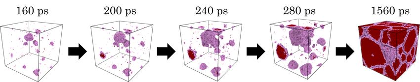
II.     UNSUPERVISED LEARNING BASED ON TOPOLOGICAL DESCRIPTORS

      We present in this section the complete methodology behind our unsupervised protocol
by describing all steps necessary to its implementation.

      A.   Data production

      This unsupervised learning approach is illustrated on pure Zr simulations. All the sim-
ulations mentioned in this paper have been performed with the lammps code [22], in the
isobaric-isothermal ensemble with help of a Nosé-Hoover thermostat and barostat [23] and
interatomic interaction describe by the MEAM potential [24] developed in [21]. The posi-
tions have been integrated through the Verlet’s algorithm in its velocity form, with a time
step of 2 fs. In order to access the inherent structures, a minimization of the energy by
means of a conjugate gradient algorithm implemented in lammps is used to bring the sys-
tem to a local minimum on the potential energy surface for each configuration wielded with
our method.
      To construct a learning model with solid and liquid structural information, a configuration
with N = 1 024 000 atoms is extracted in the course of nucleation from the nose of the time-
temperature-transformation (TTT) curve at T = 1250 K and constant ambient pressure as
reproduced in Fig. 1 from [21]. The average nucleation time for each temperature of this
curve is calculated on five independant isotherms in terms of random velocity distribution,
from an initial configuration extracted from a melt quenching simulation at a cooling rate
of 1012 K/s.

      B.   Data preparation

      We consider local atomic structures in the configuration through a coordination sphere,
consisting of a central particle and its surrounding environment delimited by a cut-off radius.
The cut-off radius can be defined thanks to the radial distribution function g(r), which gives
the probability to find a particle at distance r to a particle at the origin and is defined by

                                                 N n(r)
                                        g(r) =             ,                                 (1)
                                                 V 4πr2 ∆r

                                                 3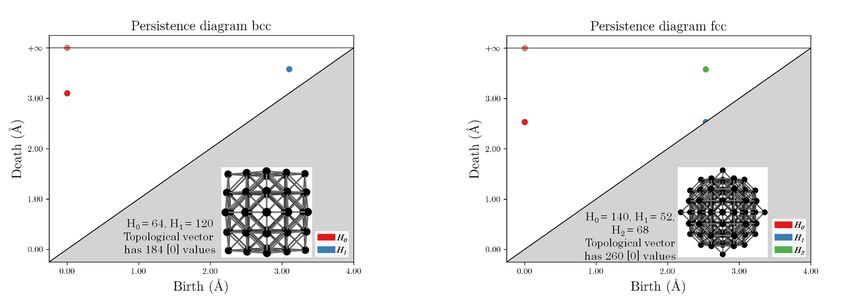
FIG. 1. Time-temperature-transformation curve with 1 024 000 atoms in a temperature range near
the nose. Inset: evolution of the potential energy as a function of time along a nucleation process.
See more details in [21].

where n(r) stands for the mean number of particles in a spherical shell of radius r and
thickness ∆r centred on the origin. A typical representation of the radial distribution
function g(r) for the liquid state of Zr is depicted in Fig. 2. Every minimum of the radial
distribution function can reasonably be used as cut-off radius to obtain local environments
which represent consecutive neighbor shells of each central particle. The first minimum
beyond the first maximum gives the end of the first neighbor shell (4.43 Å from the central
particle in Fig. 2), the second minimum, the end of second neighbor shell (7.28 Å from the
central particle) and so on.

   Among the million of particles in the configuration brought in its inherent structures,
local atomic structures are subsampled to construct a training set for the learning. To be
representative of the configuration while satisfying statistical independency, the subsampling
should pave the whole simulation box with respect to the periodic boundary conditions
(PBC). Given a cut-off radius, the subsample is one among the maximal set such that
central particles of local atomic structures are separated by at least two times this cut-off.
More precisely, such a set is defined by picking a random particle in the box from which this
cut-off criterion is iteratively redone until independant structures are established through

                                                4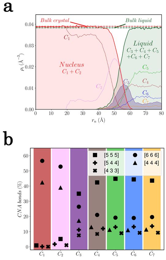
the identification of their central particle. The choice of a specific cut-off, i.e. first shell,
second shell, etc. as well as the number of structures in the set will be justified in the next
subsection.

FIG. 2. First and second neighbor shells of a central particle (in red) with cut-off radii determined
by the radial distribution function g(r) of undercooled Zirconium at 1250 K.

   Once the central particles have been identified, the Python package pyscal [25] is used
on the full configuration to extract effectively the particles coordinates of the local atomic
structures.

   C.   Persistent homology as a local atomic structure descriptor

   To encode topological informations of the local atomic structures, we use PH, a popular
TDA tool [26, 27] which detects relevant topological features from a point cloud.
   Given a set of points X, one can construct a collection of simplicial complexes [28], called
Vietoris-Rips complexes as follows. Given t ≥ 0, we consider the simplicial complex Xt which
is the union of k-simplices for k ∈ N, where 0-simplices are all the points of X, 1-simplices
are segments with extremities in X of length smaller than t, 2-simplices are full triangles

                                                5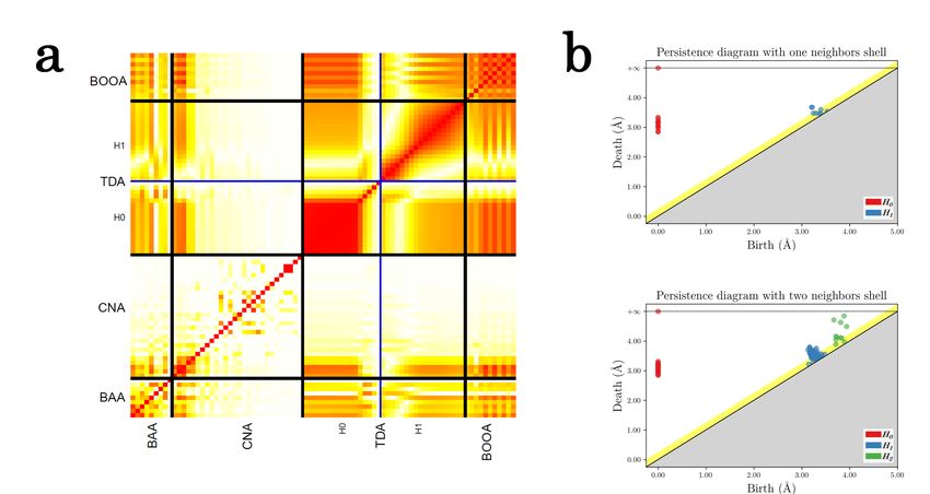
with vertices in X and distant of at most t from one another, etc. In the end, we get an
increasing sequence (called filtration) X = (Xt )t≥0 of simplicial complexes. Actually, since
the number of points is finite, changes in these complexes only appear at a finite sequence
of steps t1 < · · · < tn which gives a finite filtration of simplicial complexes X0 = Xt0 ⊂
Xt1 ⊂ · · · ⊂ Xtn . For each space Xt of the filtration, we compute the simplicial homology,
which is the sequence of their homology groups (Hk (Xt ))k≥0 , further denoted (Hk )k≥0 when
the space is understood or not specified for general consideration. The dimension of these
homology groups give insights on the dataset. A persistence diagram (PD) summarizes this
information by plotting the pair (birth, death) of each topological feature of the filtration
on a graph, as illustrated in Fig. 3. For instance, the dimension of H0 gives the number
of connected components, the dimension of H1 the number of holes and the dimension of
H2 the number of cavities inside the simplicial complex. Given a filtration of simplicial
complexes (Xt )t≥0 , one can keep track of topological features (encoded by elements in the
homology groups) and how ”persistent” they are, i.e. at which t they appear (the birth)
and at which t they disappear (the death).
   Using Python packages gudhi [29] and ripser.py [30], the individual PDs of the pre-
viously extracted train set’s local atomic structures are computed for each H0 , H1 and H2
homological dimensions. To remove the topological noise when considering H1 and H2 , we
use a subsampling approach as introduced in [31].
   While PDs are usually compared using the Bottleneck distance, their space equipped
with this metric cannot be embedded into a euclidean space nor even a normed vector space
[32]. To tackle this problem, several mapping into vector spaces have been proposed. In
this paper we use a method developed in [33] and classically used to study 3D shapes. Each
coordinate of the topological vector is associated to a pair of points (x, y) in a PD D for a
fixed level of homology, except the infinite point, and is calculated by

                         mD (x, y) = min{kx − yk∞ , d∆ (x), d∆ (y)},                      (2)

where d∆ (·) denotes the `∞ distance to the diagonal, and those coordinates are sorted by
decreasing order. Remark that the dimension of each topological vector depends on the local
atomic structure, so we fill in each vector with a non-informative value to reach the maximal
dimension of the descriptor space. Here we decided to fill the vectors with the value −1
instead of 0 as proposed in [33], as distances between points in PDs are always nonnegative,

                                             6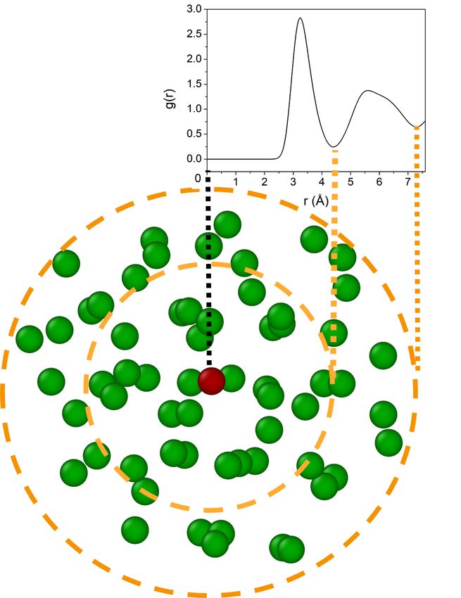
and a zero, two points of the PD with the same birth and death, corresponds to a relevant
information in our context. To highlight the importance of these zeros in our topological
vectors, let’s consider Zr atoms on a body-centered cubic (bcc) lattice up to the second
neighbor shell (7.16 Å from the central particle) and Zr atoms on a face-centered cubic (fcc)
lattice in the same shell as shown in Fig. 3. Despite these structures are fundamentally
different, one can notice that the only thing that differ between the topological vectors
obtained from each structure is the dimension of the vector (64+120 [0] values for the bcc
lattice, 140+52+68 [0] values for the fcc lattice). Thus, filling with zeros the smallest of the
two will give two identical vectors, which means the same point in the descriptor space.

FIG. 3. Left: Zr atoms on a bcc lattice and the corresponding PD. Right: Zr atoms on a fcc lattice
and the corresponding PD.

   To illustrate the relevance of our topological signature to study the local atomic struc-
tures, we confront it to widely used classical physical descriptors such as the Bond Angle
Analysis (BAA) [34], the Bond-Orientational Order Analysis (BOOA) [35] in its averaged
definition [36], and the Common Neighbor Analysis (CNA) [37] on our Zr simulation. This
classical descriptors characterize the radial and/or angular distribution of bonded pairs of
atoms in the coordination sphere. Fig. 4(a) gives an empirical correlation matrix between
the coordinates of our TDA descriptor, BAA, BOOA and CNA. This matrix is constructed
on a sample of approximately 25 000 local structures extracted as described in II B with
a cut-off corresponding to the first minimum of the radial distribution function. This last
choice was made since a descriptor like CNA cannot be applied beyond the first shell of
neighbor. The empirical correlation matrix shows that the topological signature is highly

                                               7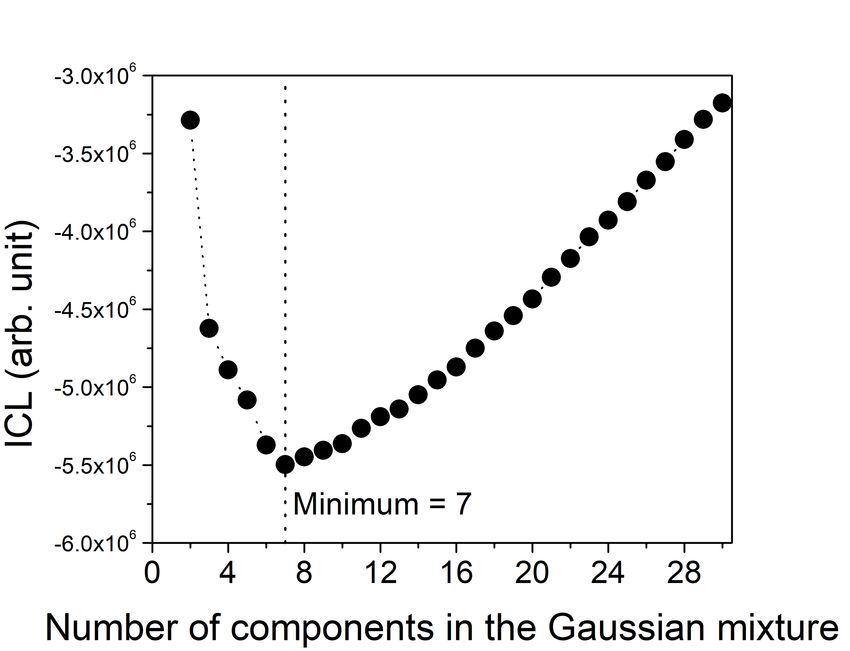
correlated with all the other descriptors. Some specificities of the data are highlighted: as
all local neighbors contain at least 10 particles, the first 10 components of H0 are highly
correlated; there are correlated with high values of H1 too, because most of the local struc-
tures have few H1 components (50 % of the population have less than 5 components); H2
components are not depicted here as there is none in local atomic structures with only the
first neighbor shell; the correlation matrix associated to the CNA is sparse, because only
few bonds, which are the first ones in the matrix (using the indexing of Faken and Jónsson
[38]: [666] and [444] for the bcc order and [555], [544] and [433] for the icosaedral order)
are present in most of the structures. It also explains the low correlation between the last
bonds in the matrix of CNA with the other descriptors.

FIG. 4. (a) empirical correlation matrix (absolute value) between several descriptor families: BAA,
CNA, TDA and BOOA. Low values are white, high values are red. We distinguish between the
descriptors by black lines, and between levels of homology with blue line (H0 and H1 ). (b) PDs of
a local atomic structure with one and two neighbor shells. Yellow line corresponds to a threshold
computed with the subsampling approach to remove noises.

   This example on the first neighbor shell illustrates how relevant signatures from H0 and
H1 are. In order to maximize the number of H0 and H1 components and also capture H2
information which appears when considering more than just one neighbor shell, we built a

                                               8
train set of 5 314 local atomic structures with two neighbor shells to construct our model.
This leads here to respectively 68, 100 and 22 of respectively H0 , H1 and H2 components
instead of only 17 H0 and 18 H1 components with one neighbor shell. Fig. 4(b) shows a
representative example of the differences in the PDs of a structure with one neighbor shell
and the same structure with two neighbor shells. The second neighbor shell play also a
crucial role in the structural description as it was highlighted [39, 40]. Therefore, this choice
allows to put a step back from first neighbor arrangements and come closer to the relevant
intermediate order. Albeit moving to higher orders shells is still possible with this persistent
homology description of the local structures, in the case of three shells of neighbor and
beyond, the benefit that we gain in topological informations is countered by too much of
an extended spatial resolution of the local structures, which leads to a loss of information
in the GMM clustering. Thus we restricted ourself to this second neighbor shell, through a
compromise between the structural informations and a coarsening of the spatial resolution,
already observed for the averaged BOOA [36].
D. Gaussian mixture model clustering
A Gaussian Mixture Model (GMM) groups data points into clusters within a unsuper-
vised way through a mixture of M Gaussian distributions (φ( · ; µm , Σm ))1≤m≤M of weights
(αm )1≤m≤M as
M
X
αm φ( · ; µm , Σm ), (3)
m=1
where µm is the mean and Σm the covariance matrix of the mth Gaussian distribution. After
a standardization of the descriptor space, an Expectation-Maximization (EM) algorithm [41]
is used as an iterative method to estimate the unknown parameters (αm , µm , Σm )1≤m≤M .
We use the implementation in the Python package scikit-learn [42] with full covariance
matrices and 3 000 K-means [43] initializations.
To select the number of Gaussian components, i.e. the number of clusters, the integrated
completed likelihood (ICL) [44] criterion has been used:
n X
X M n X
X M
ICL = −2 ln(L̂) + D ln(n) − 2 τ̂m,k ln(τ̂m,k ) = BIC − 2 τ̂m,k ln(τ̂m,k ), (4)
k=1 m=1 k=1 m=1
where L̂ denotes the likelihood evaluated on the estimator, D the number of parameters to
9be estimated (D = M (d + d2 + 1), with d the dimension of the topological vector), and τ̂m,k
denotes the probability to belong to the mth component conditionally to the observation xk .
The ICL generalizes the widely used Bayesian information criterion (BIC) [45] to clustering
methods by adding an entropy’s penalty computed from the probabilities of the data to be
assigned to each Gaussian component. The number of Gaussian components associated to
the minimum of ICL is then set as the number of clusters for the model.
III. APPLICATION OF THE UNSUPERVISED APPROACH ON ELEMENTAL
ZIRCONIUM SIMULATIONS
We focus in this section on the application of our TDA-GMM method after the building
of a model. We demonstrate then that this protocol is able to provide relevant structural
information in such a challenging context as homogeneous nucleation.
A. Learning the model
In order for the model to capture all structural atomic events of interest, the choice of a
configuration in course of nucleation where supercooled liquid coexist with crystalline nuclei
have to be made, as mentioned in subsection II A. Fig. 5 shows the ICL of the previously
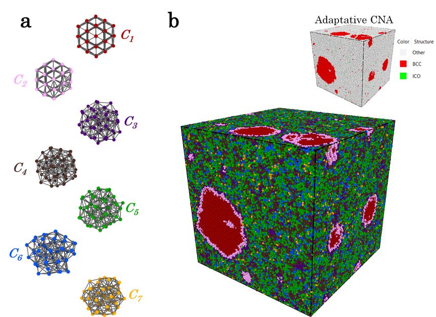
extract train set in subsection II C, leading here to 7 clusters [46]. Each cluster Ci will be
represented by the structure which is the closest to the mean of the corresponding Gaussian
component, as illustrated in Fig. 6(a).
Once the model is learned, it can be applied to new uncategorised local atomic structures
considering their topological signatures. To test the robustness of our model, we applied it
to all the remaining million of structures in the configuration which have not been included
in the train set. This new set of data is then seen as a test set in which it is remarkable
to notice that the affectations’ probabilities in the clusters are nearly always of 1: 99.998 %
of the structures have probabilities beyond 0.999 to be in one cluster of the model and the
remaining ones still have probabilities higher than 0.5. A deeper analysis of the distribution
of the test data in the descriptor space in regard to the model can also be achieved by
mean of the Mahalanobis distance (MaD) [47]. This metric is indeed able to compute the
distance between an empirical Gaussian distribution and new set of data in order to know
10FIG. 5. ICL criterion on the train set. Its minimum corresponds to the maximum of likelihood
which leads to the optimal number of clusters to build the model.
the similarities between the two sets. For each cluster and its higher probabilities structures
affected by hard-assignment, the MaD between the test data and the multivariate Gaussian
distributions of the model have been determined. Outliers are then considered based on the
interquartile range rule. Table I presents the percentage of structures in each cluster viewed
at outliers according to this criterion. More than 96 % of the structures in the test set have
a MaD in agreement with their assigned Gaussian distribution of the model.
Clusters C1 C2 C3 C4 C5 C6 C7 Total
Proportion (%) 11.70 7.22 9.28 24.45 33.46 11.03 2.86 100
Outliers (%) 2.47 2.12 6.29 3.25 3.67 3.88 3.06 3.56
TABLE I. Proportions of structures and percentage of outliers in each cluster of the test set based
on the interquartile range rule on the MaD between the test data and their assigned multivariate
Gaussian distribution of the model in the descriptor space.
The final clustering is showed on Fig. 6(b) on the entire configuration depicted in the real
space of the simulation box with help of the software ovito [48]. In inset, the classification
found by a classical adaptative CNA algorithm as implemented in ovito is represented for
comparison. As can be seen, in contrast to our method named TDA-GMM, only two types
of structures which correspond to strictly crystalline or icosahedral structures have been
successfully identified.
11FIG. 6. (a) representation in the real space of the local structures assigned to each cluster Ci . (b)
snapshot of the one million atoms in the simulation box after the clustering in the descriptor space.
In inset, the classification get with an adaptative CNA method is depicted.
B. Description of the bulks crystal and liquid
Prior to the analysis of homogenenous nucleation events from our Zr simulations, we
applied our model to a configuration with N = 128 000 atoms in the bulks crystal and
liquid at T = 1250 K. Fig. 7 and Table II shows the results obtained in the two cases
through the central atoms of the structures associated to each cluster.
For the bulk crystal, only structures from cluster C1 are identified. Referring to Fig. 6(a),
the atoms of the mean local structure associated to C1 are indeed on a periodic lattice. In
the bulk liquid, more than 99.96 % of the identified structures belong to clusters C3 to C7 .
From this simple application, and without any labels yet about the physical nature of the
atomic structures, the TDA-GMM method enables us nevertheless to distinguish solid-like
12FIG. 7. Snapshots at T = 1250 K of Zr bulks crystal (a) and liquid (b) brought in their inherent
structures. Atoms are colored according to the cluster they belong to (see Fig. 6).
Bulk Crystal Liquid
C1 (%) 100 < 0.00
C2 (%) 0 0.03
C3 (%) 0 6.49
C4 (%) 0 29.83
C5 (%) 0 45.22
C6 (%) 0 14.70
C7 (%) 0 3.72
TABLE II. Proportion of each cluster Ci in the bulks crystal and liquid.
from liquid-like clusters from the trained model.
C. Description of the homogeneous crystal nucleation
During the homogeneous nucleation process along an isotherm, the internal energy of
the system undergoes a sharp drop. It follows the growth of the nuclei that carries the
crystalline periodicity until the state of least energy is reached. To autonomously highlight
this nuclei from the clusters obtained by the TDA-GMM method, five configurations along
an isotherm at the nose of the TTT at T = 1250 K with N = 1 024 000 atoms are selected.
They go from the onset of nucleation at 160 ps from the quench up to a configuration in the
13polycrystalline bulk at 1560 ps. The model build in III A corresponds to a configuration in
the course of nucleation at 360 ps. Table III shows the evolution of the proportion of each
cluster in this configurations.
Time (ps) 160 200 240 280 310(M ) 1560(S)
C1 (%) 0.25 0.95 2.85 6.83 12.66 67.21
C2 (%) 0.67 1.37 2.76 4.96 6.85 22.65
C3 (%) 7.37 7.68 8.18 8.75 8.51 6.99
C4 (%) 29.99 29.47 28.41 26.52 24.22 1.58
C5 (%) 43.69 42.87 40.99 37.42 33.78 0.90
C6 (%) 14.44 14.14 13.48 12.36 11.16 0.35
C7 (%) 3.59 3.53 3.32 3.15 2.82 0.31
TABLE III. Proportion of each cluster Ci at different times of the nucleation process. Superscripts
(M) and (S) correspond respectively to the configuration used to train the model and the solidified
configuration.
As it can be seen, structures from clusters C1 and C2 follow a fast growth until they are
the majority in the final bulk. On the contrary, the other clusters undergo a more or less
strong decrease of their proportions through time. As mentioned in the previous subsection
III B, structures from C1 corresponds to a crystalline order whereas atoms of the mean local
structure associated to C2 are on a partial periodic lattice. Fig. 8 represents the snapshots
of this clusters in the several configurations. One can also notice that the multiplicity of
the other clusters classified as liquid shows that outside the nuclei, there exists complex
structural heterogeneities in the supercooled liquid, which we develop in the last subsection,
and which are successfully highlighted by the TDA-GMM method. Such an assessment
have been recently brought out too in supercooled liquid mixtures by another unsupervised
method based on an information-theoretic approach [12].
To extract the independent nuclei formed by structures from C1 and/or C2 , a distance-
based neighboring criterion as implemented in ovito is used to define sets of connected
particles. This criterion is set as the first minimum of g(r) in such a manner that two
particles are connected if they are at a distance less than or equal to this threshold. The
size distributions of this independent nuclei is then obtain by accounting all atoms of the
14FIG. 8. Snapshots of Zr’s configurations along nucleation at the nose of the TTT at T = 1250
K. The structures in the clusters C1 and C2 identified as carrying the crystalline periodicity are
respectively depicted through their central particle in red and pink.
overlapping local atomic structures of two neighbor shells defined by each central particle
belonging to C1 and/or C2 . The critical size is estimated by the smallest cluster which
persists through the several configurations of nucleation with at least the same number of
atoms, which leads to the current high undercooling regime to a critical nucleus size of 70-80
atoms.
D. Translational and orientational orderings
Two physical orderings which have been shown to be important parameters driving nu-
cleation are the translational and orientational orderings [49–51].
With the nuclei extracted, their centers of mass are easily inferred. Based on these
positions, the spatial evolution of the translational order from the nuclei to the liquid can
be quantified through the density. The density is indeed the dedicated indicator to measure
the fluctuations in the relative positions of neighboring atoms: for each cluster Ci and its
relative number of atoms Ki (rn ) in a spherical shell of volume Vs extending from the center
of a nucleus to a distance rn to (rn + ) with = 1 Å, the radial partial atomic density
profiles ρi (rn ) are computed as:
Ki (rn ) 4
ρi (rn ) = , with Vs = π[(rn + )3 − rn3 ]. (5)
Vs 3
On the other hand, the analysis of the orientational order provides information on the
fluctuations in the relative geometrical bonds between neighboring atoms. The CNA, follow-
ing the indexing of Faken and Jónsson, is then performed in each cluster as a representative
measure [52].
15This ordering analysis on the Zr’s nuclei showed us a general behavior, even for the
precritical ones, which is depicted for the two orderings in Fig. 9.
FIG. 9. (a) Representation on a nucleus of the typical translational ordering of the nuclei and
their surrounding liquid through the radial density profile of the Ci clusters. The corresponding
densities of the bulks crystalline and undercooled liquid have been determined at T = 1250 K and
constant ambient pressure. This behavior of the translational order is representative of all nuclei
in the configurations, even the precritical ones. (b) Typical orientationnal order of the Ci clusters
in the configurations through CNA.
16Fig. 9(a) reveals that all the nuclei emerge with a translational order which corresponds
to the density of the bulk crystal. Despite the small density window between the crystalline
and bulk liquid, it is clearly spotted that the sum of the respective densities ρi of the clusters
Ci associated to the nuclei or liquid leads to the density of the corresponding bulk. Fig. 9(b)
confirms the crystalline structures in C1 and C2 which exhibit bcc bonds ([666]: 8, [444]:
6) and so a concurrent emergence of the orientational order in the nucleation process. The
slight percentage of icosahedral bonds [555] in C2 tends to explain the partial periodicity
observed on Fig. 6(a). On the other side, structures from clusters C4 to C7 share strong
five-fold symmetries bonds characteristics of the undercooled liquid, although they possess
also non-negligible relative bcc bonds. From them, about 4 % of [666] in each cluster are in
excess to form a bcc structures and have the possibilities to combine with the [555] bonds in
Frank-Kasper polyhedra Z14, Z15 and Z16 [53]. This can lead to a geometrical frustration
able to slow down the onset of the nucleation in the liquid part [54, 55]. At last, C3 is
more a peculiar case with a strong distribution at the border of nuclei while also presents in
the deeper liquid. Its presence in the frontier region is explained by the spatial resolution
already mentioned in II C, while its presence in the liquid can be seen as precursors for the
embryos emergence. This is in agreement with the latest view of an heterogeneous scenario
in which precursors of the crystalline order arise from structural heterogeneities in the liquid
[56–58] and which we develop in the next subsection.
There is no consensus in the literature for a general pathway of the nucleation process of
materials, which seems to be system dependent: hard spheres systems undergo concurrent
translational and orientational ordering [51], while a decoupling of this two symmetries have
been observed in colloidal systems [49]. For a pure metal like Zr, our unsupervised analysis
brings us to the conclusion that translational and orientational orders arise synchronously.
E. Liquid heterogeneities
To assess the scenario mentioned in the previous subsection, heterogeneity at an early
nucleation stage is evaluated by a comparison of the distribution of atoms belonging to each
cluster against the uniform distribution. As comparison of distributions are particularly
complex in 3 dimensions as the empirical cumulative distribution function is not defined,
a Kolmogorov-Smirnov (KS) test [59] have been performed on the projection of atomic
17positions on the 3 directions of space. For a level 0.01, if the uniform distribution is rejected
on at least a projection, it is rejected for the multivariate dataset. Table IV depicts the
results through the p-values of the test obtained from the configuration at 160 ps. For all
the clusters, the test is always rejected, meaning that the distribution of the clusters is not
uniform, in other words, their heterogeneities in the simulation box.
p-value x y z
C1 0.000 0.000 0.000
C2 0.000 0.000 0.000
C3 0.000 0.000 0.000
C4 0.000 0.000 0.007
C5 0.001 0.000 0.000
C6 0.007 0.331 0.001
C7 0.192 0.156 0.005
TABLE IV. p-values computed on the projection of atomic positions at an early nucleation stage
(160 ps) on each direction of the simulation box from a KS test against the uniform distribution.
IV. CONCLUSIONS
We reported a method for the structural analysis of materials at the atomic scale based
on the unsupervised clustering provided by a Gaussian Mixture Model run on topological
descriptors build on the atomic positions of local atomic structures. The originality of the
use of persistent homology as atomic descriptors lead to an autonomous identification of
clusters of singular structures by return to the real space of the box. We used this without a
priori approach for the analysis of several MD configurations of Zr in the challenging context
of homogeneous nucleation and highlighted some interesting properties of the phenomenon.
A deeper look of the nucleation process of other pure metals have been investigated through
this TDA-GMM method and the results will be published soon.
This unsupervised approach opens the door to application to more structural dependent
phenomena at the atomic scale. Extension of the analysis on multicomponent systems where
chemical orders arise is also especially relevant for a deeper inspection and control of such
18mechanisms to enhance materials design.
ACKNOWLEDGEMENT
We acknowledge the CINES and IDRIS under Project No. INP2227/72914, as well
as CIMENT/GRICAD for computational resources. This work was performed within
the framework of the Centre of Excellence of Multifunctional Architectured Materials
“CEMAM”ANR-10-LABX-44-01 funded by the “Investments for the Future” Program.
This work has been partially supported by MIAI@Grenoble Alpes (ANR-19-P3IA-0003).
Fruitful discussions within the French collaborative network in high-temperature thermo-
dynamics GDR CNRS3584 (TherMatHT) are also acknowledged.
[1] G. C. Sosso, J. Chen, S. J. Cox, M. Fitzner, P. Pedevilla, A. Zen, and A. Michaelides, Chem.
Rev. 116, 7078 (2016).
[2] D. Frenkel and B. Smit, Understanding Molecular Simulation: From Algorithms to Applica-
tions. 2nd Ed, Vol. 50 (1996).
[3] T. Hey, S. Tansley, and K. Tolle, The Fourth Paradigm: Data-Intensive Scientific Discovery
(Microsoft Research, 2009).
[4] P. Geiger and C. Dellago, The Journal of Chemical Physics 139, 164105 (2013).
[5] C. Dietz, T. Kretz, and M. H. Thoma, Phys. Rev. E 96, 011301 (2017).
[6] E. Boattini, M. Ram, F. Smallenburg, and L. Filion, Molecular Physics 116, 3066 (2018).
[7] R. S. DeFever, C. Targonski, S. W. Hall, M. C. Smith, and S. Sarupria, Chem. Sci. 10, 7503
(2019).
[8] W. F. Reinhart, A. W. Long, M. P. Howard, A. L. Ferguson, and A. Z. Panagiotopoulos, Soft
Matter 13, 4733 (2017).
[9] W. F. Reinhart and A. Z. Panagiotopoulos, Soft Matter 14, 6083 (2018).
[10] M. Ceriotti, J. Chem. Phys. 150, 150901 (2019).
[11] E. Boattini, M. Dijkstra, and L. Filion, J. Chem. Phys. 151, 154901 (2019).
[12] J. Paret, R. L. Jack, and D. Coslovich, J. Chem. Phys. 152, 144502 (2020).
[13] M. Spellings and S. C. Glotzer, AIChE Journal 64, 2198 (2018).
19[14] F. C. Motta, in Advances in Nonlinear Geosciences, edited by A. A. Tsonis (Springer Inter-
national Publishing, Cham, 2018), pp. 369–391.
[15] H. Tanaka, H. Tong, R. Shi, and J. Russo, Nat Rev Phys 1, 333 (2019).
[16] T. Nakamura, Y. Hiraoka, A. Hirata, E. G. Escolar, and Y. Nishiura, Nanotechnology 26,
304001 (2015).
[17] Y. Hiraoka, T. Nakamura, A. Hirata, E. G. Escolar, K. Matsue, and Y. Nishiura, Proc Natl
Acad Sci USA 113, 7035 (2016).
[18] A. Hirata, T. Wada, I. Obayashi, and Y. Hiraoka, Commun Mater 1, 98 (2020).
[19] S. Hong and D. Kim, J. Phys.: Condens. Matter 31, 455403 (2019).
[20] K. Sasaki, R. Okajima, and T. Yamashita, Liquid Structures Characterized by a Combina-
tion of the Persistent Homology Analysis and Molecular Dynamics Simulation (Thessaloniki,
Greece, 2018), p. 020015.
[21] S. Becker, E. Devijver, R. Molinier, and N. Jakse, Phys. Rev. B 102, 104205 (2020).
[22] S. J. Plimpton, J. Comput. Phys.117, 1 (1995).
[23] M. P. Allen and D. J. Tildesley, Computer Simulation of Liquids: Second Edition, Oxford
Science Publication (Oxford University Press, Oxford, 2017).
[24] M. I. Baskes, Phys. Rev. B 46, 2727 (1992).
[25] S. Menon, G. Leines, and J. Rogal, JOSS 4, 1824 (2019).
[26] H. Edelsbrunner, D. Letscher, and A. Zomorodian, Discrete Comput Geom 28, 511 (2002).
[27] A. Zomorodian and G. Carlsson, Discrete Comput Geom 33, 249 (2005).
[28] R. Ghrist, Bull. Amer. Math. Soc. 45, 61 (2007).
[29] C. Maria, J.-D. Boissonnat, M. Glisse, M. Yvinec. ”The Gudhi Library: Simplicial Complexes
and Persistent Homology”, Mathematical Software, ICMS, 167-174, 2014.
[30] C. Tralie, N. Saul, and R. Bar-On, JOSS 3, 925 (2018).
[31] B. T. Fasy, F. Lecci, A. Rinaldo, L. Wasserman, S. Balakrishnan, and A. Singh, Ann. Statist.
42, (2014).
[32] M. Carrière and U. Bauer, 35th International Symposium on Computational Geometry, 21,
(2019).
[33] M. Carrière, S. Y. Oudot, and M. Ovsjanikov, Computer Graphics Forum 34, 1 (2015).
[34] G. J. Ackland and A. P. Jones, Phys. Rev. B 73, 054104 (2006).
[35] P. J. Steinhardt, D. R. Nelson, and M. Ronchetti, Phys. Rev. B 28, 784 (1983).
20[36] W. Lechner and C. Dellago, The Journal of Chemical Physics 129, 114707 (2008).
[37] J. D. Honeycutt and H. C. Andersen, J. Phys. Chem. 91, 4950 (1987).
[38] D. Faken and H. Jónsson, Computational Materials Science 2, 279 (1994).
[39] A. K. Soper and M. A. Ricci, Phys. Rev. Lett. 84, 2881 (2000).
[40] Z. Yan, S. V. Buldyrev, P. Kumar, N. Giovambattista, P. G. Debenedetti, and H. E. Stanley,
Phys. Rev. E 76, 051201 (2007).
[41] A. P. Dempster, N. M. Laird, and D. B. Rubin, Journal of the Royal Statistical Society: Series
B (Methodological) 39, 1 (1977).
[42] F. Pedregosa, G. Varoquaux, A. Gramfort, V. Michel, B. Thirion, O. Grisel, M. Blondel, P.
Prettenhofer, R. Weiss, V. Dubourg, J. Vanderplas, A. Passos, and D. Cournapeau, JMLR
12, 2825 (2011).
[43] S. Lloyd, IEEE Trans. Inform. Theory 28, 129 (1982).
[44] C. Biernacki, G. Celeux, and G. Govaert, IEEE Trans. Pattern Anal. Machine Intell. 22, 719
(2000).
[45] G. Schwarz, The Annals of Statistics 6, 461 (1978).
[46] See Supplemental Material for boxplots of the topological vectors in the homological dimen-
sions H0 , H1 and H2 for each cluster Ci .
[47] P. C. Mahalanobis, Proceedings of the National Institute of Sciences (Calcutta) 2, 49 (1936).
[48] A. Stukowski, Modelling Simul. Mater. Sci. Eng. 18, 015012 (2010).
[49] J. Russo and H. Tanaka, Sci Rep 2, 505 (2012).
[50] J. Russo and H. Tanaka, J. Chem. Phys. 18 (2016).
[51] J. T. Berryman, M. Anwar, S. Dorosz, and T. Schilling, The Journal of Chemical Physics 145,
211901 (2016).
[52] N. Jakse and A. Pasturel, Phys. Rev. Lett. 91, 195501 (2003).
[53] D. R. Nelson and F. Spaepen, Solid State Physics, Vol. 42 (Elsevier, 1989), pp. 1–90.
[54] H. Tanaka, Eur. Phys. J. E 35, 113 (2012).
[55] J. Russo, F. Romano, and H. Tanaka, Phys. Rev. X 8, 021040 (2018).
[56] A. Pasturel and N. Jakse, Npj Comput Mater 3, 33 (2017).
[57] Y. Shibuta, S. Sakane, E. Miyoshi, S. Okita, T. Takaki, and M. Ohno, Nat Commun 8, 10
(2017).
[58] G. Jug, A. Loidl, and H. Tanaka, EPL 133, 56002 (2021).
21[59] A. Kolmogoroff, Giornale dell’Istituto Italiano degli Attuari 4, (1933).
Supplemental Material
BOXPLOTS OF THE DESCRIPTORS FOR EACH CLUSTER OBTAINED BY
THE TDA-GMM METHOD ON ELEMENTAL ZR
Cluster 1
FIG. S10. Boxplots of the topological vectors in homological dimension H0 for data in C1 .
22FIG. S11. Boxplots of the topological vectors in homological dimension H1 for data in C1 .
FIG. S12. Boxplots of the topological vectors in homological dimension H2 for data in C1 .
23Cluster 2
FIG. S13. Boxplots of the topological vectors in homological dimension H0 for data in C2 .
FIG. S14. Boxplots of the topological vectors in homological dimension H1 for data in C2 .
24FIG. S15. Boxplots of the topological vectors in homological dimension H2 for data in C2 .
Cluster 3
FIG. S16. Boxplots of the topological vectors in homological dimension H0 for data in C3 .
25FIG. S17. Boxplots of the topological vectors in homological dimension H1 for data in C3 .
FIG. S18. Boxplots of the topological vectors in homological dimension H2 for data in C3 .
26Cluster 4
FIG. S19. Boxplots of the topological vectors in homological dimension H0 for data in C4 .
FIG. S20. Boxplots of the topological vectors in homological dimension H1 for data in C4 .
27FIG. S21. Boxplots of the topological vectors in homological dimension H2 for data in C4 .
Cluster 5
FIG. S22. Boxplots of the topological vectors in homological dimension H0 for data in C5 .
28FIG. S23. Boxplots of the topological vectors in homological dimension H1 for data in C5 .
FIG. S24. Boxplots of the topological vectors in homological dimension H2 for data in C5 .
29Cluster 6
FIG. S25. Boxplots of the topological vectors in homological dimension H0 for data in C6 .
FIG. S26. Boxplots of the topological vectors in homological dimension H1 for data in C6 .
30FIG. S27. Boxplots of the topological vectors in homological dimension H2 for data in C6 .
Cluster 7
FIG. S28. Boxplots of the topological vectors in homological dimension H0 for data in C7 .
31FIG. S29. Boxplots of the topological vectors in homological dimension H1 for data in C7 .
FIG. S30. Boxplots of the topological vectors in homological dimension H2 for data in C7 .
32You can also read