Accurate Camera Calibration from Multi-View Stereo and Bundle Adjustment
←
→
Page content transcription
If your browser does not render page correctly, please read the page content below
International Journal of Computer Vision manuscript No.
(will be inserted by the editor)

Accurate Camera Calibration from Multi-View Stereo and Bundle
Adjustment
Yasutaka Furukawa · Jean Ponce

Received: date / Accepted: date

Abstract The advent of high-resolution digital cameras and              1 Introduction
sophisticated multi-view stereo algorithms offers the promise
of unprecedented geometric fidelity in image-based model-               Modern multi-view stereovision (MVS) systems are capa-
ing tasks, but it also puts unprecedented demands on camera             ble of capturing dense and accurate surface models of com-
calibration to fulfill these promises. This paper presents a            plex objects from a moderate number of calibrated images:
novel approach to camera calibration where top-down infor-              Indeed, a recent study has shown that several algorithms
mation from rough camera parameter estimates and the out-               achieve surface coverage of about 95% and depth accuracy
put of a multi-view-stereo system on scaled-down input im-              of about 0.5mm for an object 10cm in diameter observed
ages is used to effectively guide the search for additional im-         by 16 low-resolution (640 × 480) cameras. Combined with
age correspondences and significantly improve camera cali-              the emergence of affordable, high-resolution (10Mpixel and
bration parameters using a standard bundle adjustment algo-             higher) consumer-grade cameras, this technology promises
rithm (Lourakis and Argyros, 2008). The proposed method                 even higher, unprecedented geometric fidelity in image-based
has been tested on six real datasets including objects without          modeling tasks, but puts tremendous demands on the cali-
salient features for which image correspondences cannot be              bration procedure used to estimate the intrinsic and extrinsic
found in a purely bottom-up fashion, and objects with high              camera parameters, lens distortion coefficients, etc.
curvature and thin structures that are lost in visual hull con-             There are two main approaches to the calibration prob-
struction even with small errors in camera parameters. Three            lem: The first one, dubbed chart-based calibration (or CBC)
different methods have been used to qualitatively assess the            in the rest of this presentation, assumes that an object with
improvements of the camera parameters. The implementa-                  precisely known geometry (the chart) is present in all in-
tion of the proposed algorithm is publicly available at (Fu-            put images, and computes the camera parameters consistent
rukawa and Ponce, 2008b).                                               with a set of correspondences between the features defin-
                                                                        ing the chart and their observed image projections (Bouguet,
                                                                        2008; Tsai, 1987). It is often used in conjunction with posi-
Keywords Bundle Adjustment · Structure from Motion ·
                                                                        tioning systems such as a robot arm (Seitz et al, 2006) or a
Multi-View Stereo · Image-Based Modeling · Camera
                                                                        turntable (Hernández Esteban and Schmitt, 2004) that can
Calibration.
                                                                        repeat the same motion with high accuracy, so that object
                                                                        and calibration chart pictures can be taken separately but
Y. Furukawa
                                                                        under the same viewing conditions. The second approach to
Box 352350, Seattle, WA 98195-2350, USA                                 calibration is structure from motion (SFM), where both the
Computer Science & Engineering                                          scene shape (structure) and the camera parameters (motion)
University of Washington                                                consistent with a set of correspondences between scene and
E-mail: furukawa@cs.washington.edu
                                                                        image features are estimated (Hartley and Zisserman, 2004).
J. Ponce                                                                In this process, the intrinsic camera parameters are often
45, rue D’Ulm, 75230 Paris Cedex 05, France
                                                                        supposed to be known a priori (Nister, 2004), or recovered
Willow project-team at the Laboratoire d’Informatique de l’Ecole Nor-
male Supérieure, ENS/INRIA/CNRS UMR 8548                               a posteriori through auto-calibration (Triggs, 1997). A final
E-mail: Jean.Ponce@ens.fr                                               bundle adjustment (BA) stage is then typically used to fine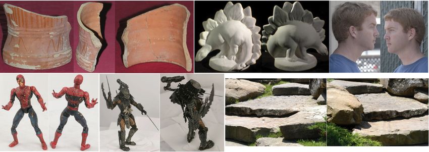
2

tune the positions of the scene points and the entire set of              ically require special equipment and software that are un-
camera parameters (including the intrinsic ones and possibly              fortunately not available in many academic and industrial
the distortion coefficients) in a single non-linear optimiza-             settings. Our goal, in this article, is to develop a flexible
tion (Lourakis and Argyros, 2008; Triggs et al, 2000). A key              but high-accuracy calibration system that is affordable and
ingredient of both approaches to calibration is the selection             accessible to everyone. To this end, a few researchers have
of feature correspondences (SFC), procedure that may be                   proposed using scene information to refine camera calibra-
manual or (partially or totally) automated, and is often inter-           tion parameters: Lavest et al. propose (1998) to compensate
twined with the calibration process: In a typical SFM system              for the inaccuracy of a calibration chart by adjusting the 3D
for example, features may first be found as “interest points”             position of the markers that make it up, but this requires
in all input images, before a robust matching technique such              special markers and software for locating them with suf-
as RANSAC (Fischler and Bolles, 1981) is used to simulta-                 ficient sub-pixel precision. The calibration algorithms pro-
neously estimate a set of consistent feature correspondences              posed in (Hernández Esteban et al, 2007) and (Wong and
and camera parameters. Some approaches propose to im-                     Cipolla, 2004) exploit silhouette information instead. They
prove feature correspondences for robust camera calibration               work for objects without any texture and are effective in
(Quan, 1995; Martinec and Pajdla, 2007). However, reliable                wide-baseline situations, but are limited to circular camera
automated SFC/SFM systems are hard to come by, and they                   motions.
may fail for scenes composed mostly of objects with weak
textures (e.g., human faces). In this case, manual feature se-                In this article, we propose a very simple and efficient BA
lection and/or CBC are the only viable alternatives.                      algorithm that does not suffer from these limitations and ex-
    Today, despite decades of work and a mature technology,               ploits top-down information provided by a rough surface re-
putting together a complete and reliable calibration pipeline             construction to establish image correspondences. Concretely,
thus remains non-trivial procedure requiring much know-                   given a set of input images, possibly inaccurate camera pa-
how, with various pitfalls and sources of inaccuracy. Auto-               rameters that may have been obtained by an SFM or CBC
mated SFC/SFM methods tend to work well for close-by                      system, and some conservative estimate of the correspond-
cameras in controlled environments—though errors tend to                  ing reprojection errors, the input images are first scaled down
accumulate for long-range motions, and they may be inef-                  so these errors become small enough to successfully run a
fective for poorly textured scenes and widely separated in-               patch-based multi-view stereo algorithm (PMVS; Furukawa
put images. CBC systems can be used regardless of scene                   and Ponce, 2007) that reconstructs a set of oriented points
texture and view separation, but it is difficult to design and            (points plus normals) densely covering the surface of the ob-
build accurate calibration charts with patterns clearly visi-             served scene, and identifies the images where they are vis-
ble from all views. This is particularly true for 3D charts               ible. The core component of the approach proposed in this
(which are desirable for uniform accuracy over the visible                paper is its second stage, where image features are matched
field), but remains a problem even for printed planar grids               across multiple views using the estimated surface geometry
(the plates the paper is laid on may not be quite flat, laser             and visibility information. Finally, matched features are in-
printers are surprisingly inaccurate, etc.). In addition, the             put to the SBA bundle adjustment software (Lourakis and
robot arms or turntables used in many experimental setups                 Argyros, 2008) to tighten up camera parameters. Besides
may not be exactly repetitive. In fact, even a camera attached            improving camera calibration, the proposed method can sig-
to a sturdy tripod may be affected during experiments by                  nificantly speed up SFM systems by running the SFM soft-
vibrations from the floor, thermal effects, etc. These seem-              ware on scaled-down input images, then using the proposed
ingly minor factors may not be negligible for modern high-                algorithm on full-resolution images to tighten-up camera cal-
resolution cameras, 1 and they limit the effectiveness of clas-           ibration. The proposed method has been tested on various
sical chart-based calibration. Of course, sophisticated setups            real datasets, including objects without salient features for
that are less sensitive to these difficulties have been devel-            which image correspondences cannot be found in a purely
oped by photogrammeters (Uffenkamp, 1993), but they typ-                  bottom-up fashion, and objects with high-curvature and thin
                                                                          structures that are lost in the construction of visual hulls
  1 For example, the robot arm (Stanford spherical gantry) used in the    without our bundle adjustment procedure (Section 4). In sum-
multi-view stereo evaluation of (Seitz et al, 2006) has an accuracy of    mary, the contributions of the proposed approach can be de-
0.01◦ for a 1m radius sphere observing an object about 15cm in diam-      scribed as follows:
eter, which yields approximately 1.0[m] × 0.01 × π /180 = 0.175[mm]
errors near an object. Even with the low-resolution 640 × 480 cameras     • Better feature localization by taking into account surface
used in (Seitz et al, 2006), where a pixel covers roughly 0.25mm on the
                                                                          geometry estimations.
surface of an object, this error corresponds to 0.175/0.25 = 0.7pixels,
which is not negligible. If one used a high-resolution 4000 × 3000
camera, the positioning error would increase to 0.7 × 4000/640 =          • Better coverage and dense feature correspondences by ex-
4.4pixels.                                                                ploiting surface geometry and visibility information.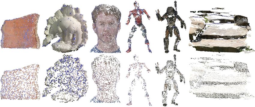
3

                            P1                           V1={1,2,3}                Input: Cameras parameters {Kj , R j ,t j } and
                                                         V2={1,2}                         expected reprojection error Er .
                 P2                                      V3={2,3}                  Output: Refined cameras parameters {Kj , R j ,t j }.

      p11
                                       P3                                          Build image pyramids for all the images.
                                            p13        Structure: Pi               Compute a level L to run PMVS: L ← max(0, log2 Er ).
                       p12
     p21                                            C3 Motion: Cj                  Repeat four times
                                              p33                                    • Run PMVS on level L of the pyramids to obtain patches
            C1                                         Observation: pij                {Pi } and their visibility information {Vi }.
                      p22        p32
                                       C2              Visibility: Vi                • Initialize feature locations: pi j ← F(Pi , {K j , R j ,t j }).
                                                                                     • Sub-sample feature correspondences.
Fig. 1 Notation: Three points P1 , P2 , P3 are observed by three cameras             • For each feature correspondence {pi j | j ∈ Vi }
C1 ,C2 ,C3 . Pi j is the image projection of Pi in C j . Vi is a set of indexes         – Identify a reference camera Cj0 in Vi with the
of cameras in which Pi is visible.                                                        minimum foreshortening factor.
                                                                                        – For each non-reference feature pi j ( j ∈ Vi , j = j0 )
                                                                                           • For L∗ ← L down to 0
                                                                                              – Use level L∗ of image pyramids to refine pi j :
• An ability to handle objects with very weak textures and                                         pi j ← argmax pi j NCC(qi j , qi j0 ).
resolve accumulation errors, two difficult issues for existing                          – Filter out features that have moved too much.
                                                                                     • Refine {Pi , K j , R j ,t j } by a standard BA with {pi j }.
SFM and BA algorithms.                                                               • Update Er by the mean and std of reprojection errors.
The rest of this article is organized as follows. Section 2
presents our imaging model together with some notations,                          Fig. 2 Overall algorithm.
and briefly introduce the MVS algorithm used in the arti-
cle (Furukawa and Ponce, 2008c). Section 3 details the pro-
posed algorithm. Experimental results and discussions are
given in Sect. 4. Note that PMVS (Furukawa and Ponce,                             where Vi encodes visibility information as the set of indices
2008c), SBA (Lourakis and Argyros, 2008), and several CBC                         of images where Pi is visible. Unlike BA algorithms, multi-
systems such as (Bouguet, 2008) are publicly available. Bun-                      view stereo algorithms are aimed at recovering scene in-
dled with our software, which is also available online at (Fu-                    formation alone given fixed camera parameters. In our im-
rukawa and Ponce, 2008b), they make a complete software                           plementation, we use the PMVS software (Furukawa and
suite for high-accuracy camera calibration. A preliminary                         Ponce, 2007, 2008c) that generates a set of oriented points
version of this article appeared in (Furukawa and Ponce,                          Pi , together with the corresponding visibility information V i .
2008a).                                                                           We have chosen PMVS because (1) it is one of the best
                                                                                  MVS algorithms to date according to the Middlebury bench-
                                                                                  marks (Seitz et al, 2006), (2) our method does not require a
                                                                                  3D mesh model but just a set of oriented points, which is the
2 Imaging Model and Preliminaries
                                                                                  output of PMVS, and (3) as noted earlier, PMVS is freely
Our approach to camera calibration accommodates in princi-                        available (Furukawa and Ponce, 2008c). This is also one of
ple any parametric projection model of the form p = f (P,C),                      the reasons for choosing the SBA software (Lourakis and
where P denotes both a scene point and its position in some                       Argyros, 2008) for bundle adjustment, the others being its
fixed world coordinate system, C denotes both an image and                        flexibility and efficiency.
the corresponding vector of camera parameters, and p de-
notes the projection of P into the image. In practice, our im-
plementation is currently limited to a standard perspective
projection model where C records five intrinsic parameters
                                                                                  3 Algorithm
and six extrinsic ones. Distortion is thus supposed to be neg-
ligible, or already corrected, for example by software such
as DxO Optics Pro (DXO, 2008). Standard BA algorithms                             The overall algorithm is given in Fig. 2. We first use the
take the following three data as inputs: a set of n 3D point                      oriented points Pi (i = 1, . . . , n) and the corresponding visi-
positions P1 , P2 , · · · , Pn , m camera parameters C1 , . . . ,Cm , and         bility information Vi output by PMVS to form initial image
the positions of the projections p i j of the points Pi in the im-                correspondences p i j , then refine these parameters p i j and
ages C j where they are visible (Fig. 1). They optimize both                      Vi by simple local image texture comparison in the second
the scene Pi and camera parameters C j by minimizing, for                         step. Given the refined image correspondences, it is possi-
example, the sum of squared reprojection errors:                                  ble to rely on SBA to improve the camera parameters. The
                                                                                  entire process is repeated a couple of times to tighten up the
 n
                                                                                  camera calibration. In this section, we will explain how to
∑ ∑ (pi j − f (Pi ,C j ))2 ,                                              (1)
                                                                                  initialize and refine feature correspondences.
i=1 j∈Vi
4
3.1 Initializing Feature Correspondences
Pi Qi
In practice, we have found PMVS to be robust to errors in pi1
camera parameters as long as the image resolution matches pi3
the corresponding reprojection errors—that is, when fea- pi2 qi3 C3
tures to be matched are roughly within two pixels of the qi1
C1 qi2
corresponding 3D points. Given an initial set of camera pa- C2
rameters, it is usually possible to obtain a conservative esti-
mate of the expected reprojection error E r by hand (e.g., by Fig. 3 Given a patch (Pi , Qi ) and the visibility information Vi , we ini-
visually inspecting a number of epipolar lines) or automat- tialize matching images patches (pi j , qi j ).
ically (e.g., by directly measuring reprojection errors asso-
ciated with the features matched by a SFM system). Thus,
we first build image pyramids for all the input images, then (Furukawa and Ponce, 2007), a patch Q i is represented by a
run PMVS on the level L = log 2 Er of the pyramids. At δ × δ grid of 3D points and the local image texture inside q i j
this level, images are 2 L times smaller than the originals, is, in turn, represented by a set of pixel colors at their image
with reprojection errors of at most about two pixels. We then projections.
project the points Pi output by this program into the images Next, our problem is to refine feature locations by match-
where they are visible to obtain an initial set of image cor- ing local image textures q i j . For efficiency, we fix the shapes
respondences p i j = f (Pi ,C j ), with j in Vi . Depending on the of the image patches q i j and only allow the positions of
value of L and the choice of the PMVS parameter ζ that con- their centers to change. This is not a problem because, as
trols the density of oriented points it constructs, the number explained later, we iterate the whole procedure a couple of
of these points, and thus, the number of feature correspon- times and the shapes of the image patches improve over iter-
dences may become quite large. Dense reconstruction is not ations. Let us call the camera with the minimum foreshort-
necessary for bundle adjustment, and we sub-sample fea- ening factor with respect to Pi the reference camera of Pi , and
ture correspondences for efficiency. 2 More concretely, we use j0 to denote its index. We fix the location p i j0 in the ref-
first divide each image into 10 × 10 uniform blocks, and ran- erence camera and optimize every other element p i j , j = j0
domly select within each block at most ε features. A feature one by one by maximizing the consistency between q i j0 and
correspondence will be used in the next refinement step if qi j in a multi-scale fashion. More concretely, starting from
at least one of its associated image features p i j was sampled the level L of the image pyramids where PMVS was used, a
in the above procedure. In practice, ε is chosen so that the conjugate gradient method is used to optimize p i j by max-
number of feature correspondences becomes ten to twenty imizing the normalized cross correlation between q i j0 and
percents of the original one after this sampling step. Note qi j . The process is repeated after convergence at the next
that sub-sampling is performed in each block (as opposed to lower level. After the optimization is complete at the bot-
each image) in order to ensure uniformly distributed feature tom level, we check whether p i j has not moved too much
correspondences. during the optimization. In particular, if p i j has moved more
than Er pixels from its original location, it is removed as an
outlier and Vi is updated accordingly. Having refined feature
3.2 Refining Feature Correspondences correspondences, we then use the SBA bundle adjustment
software (Lourakis and Argyros, 2008) to update the cam-
Due to the use of low-resolution images in PMVS and er- era parameters. In practice, we repeat the whole procedure
rors in camera parameters, the initial values of p i j are not (PMVS, multi-view feature matching, and SBA) four times
accurate. Therefore, the second step of the algorithm is to to tighten up the camera calibration, while E r is updated to
optimize the feature locations p i j by comparing local image be the mean plus three times the standard deviation of repro-
textures. Concretely, since we have an estimate of the sur- jection errors computed in the last step. Note that L is fixed
face normal at each point Pi , we consider a small 3D rect- across iterations instead of recomputed from E r . This is for
angular patch Q i centered at Pi and construct its projection efficiency, since PMVS runs slowly with a small value of L.
qi j in the set Vi of images where Pi is visible (Fig. 3). We
automatically determine the extent of Q i so its largest pro-
jection covers an image area of about δ × δ pixels (we have 4 Experimental Results and Discussions
used δ = 7 throughout our experiments). In practice, as in
4.1 Datasets
We could increase the value of ζ to obtain a sparser set of patches
2
without sub-sampling, but, as detailed in (Furukawa and Ponce, 2007),
a dense reconstruction is necessary for this algorithm to work well and The proposed algorithm has been implemented in C++ and
determine visibility information accurately. tested on six real datasets, with sample input images shown5
Table 1 The number of images and their approximate resolution (in the sparse manual feature correspondences (at most a few
megapixels) are listed for each dataset. Er is the expected reprojection dozens among close-by views) used to calibrate the cam-
error in pixels, L is the level of image pyramids used by PMVS, Np is
eras. The vase dataset has relatively small reprojection er-
the number of patches reconstructed by PMVS, and Nt is the number of
patches that have successfully generated feature correspondences after rors with many close-by images for which SFM algorithms
sub-sampling. work well, but some images contain large reprojection er-
# of # of rors because of the use of a flash and the limited depth of
Er L Np Nt field, and errors do accumulate. The step data set does not
images pixels
vase 21 3M 12 3 9926 1310 have these problems, but since scaled-down images are used
dino 16 0.3M 7 2 5912 1763 for the SFC/SFM/BA system, it contains some errors in full
face 13 1.5M 8 3 7347 1997
spiderman 16 1M 7 2 3344 840 resolution images. Note that since silhouette information is
predator 24 2M 7 2 12760 3587 used both by the PMVS software and the visual hull compu-
step 7 6M 5 2 106806 9500 tations described in the next section, object silhouettes have
been manually extracted using PhotoShop for all datasets
except dino, where background pixels are close to black, and
in Fig. 4, and the number of images and their (approximate) thresholding followed by morphological operations is suffi-
resolution listed in Table. 1. The vase and step datasets have cient to obtain the silhouettes. Note that the silhouette ex-
been calibrated by a local implementation (Courchay, 2007) traction is not essential for our algorithm, although it helps
of a standard automated SFC/SFM/BA suite as described the system to run and converge more quickly. Furthermore,
in (Hartley and Zisserman, 2004). For the step dataset, the the use of PMVS is not essential either and this software can
input images are scaled-down by a factor of five to speed up be replaced by any other multi-view stereo system.
the execution of the SFM software, but the full-resolution
images are used for our refinement algorithm. Our SFM im-
plementation fails on all other datasets except for predator, 4.2 Experiments
for which 14 out of the 24 images have been calibrated suc-
cessfully. It is of course possible that a different implementa- The two main parameters of PMVS are a correlation window
tion would have given better results, but we believe that this size γ , and a parameter ζ controlling the density of the re-
is rather typical of practical situations when different views construction: PMVS tries to reconstruct at least one patch in
are widely separated and/or textures are not prominent, and every ζ × ζ image window. We use γ = 7 or 9 and ζ = 2 or 4
this is a good setting to exercise our algorithm. The spi- in all our experiments. Figure 5 shows for each dataset a set
derman dataset has been calibrated using a planar checker- of patches reconstructed by PMVS (top row), and its subset
board pattern and a turntable with the calibration software that have successfully generated feature correspondences af-
from (Bouguet, 2008), and the same setup has been used ter sub-sampling (bottom row). Table 1 gives some statistics
to obtain a second set of camera parameters for the preda- on the matching procedure. E r denotes a conservative esti-
tor dataset. The face dataset was acquired outdoors, with- mate of the expected reprojection errors in pixels, and L de-
out a calibration chart, and textures are too weak for typical notes the level of image pyramids used by PMVS to recon-
automated SFC/SFM algorithms to work. This is a typical struct a set of patches. The number of patches reconstructed
case where, in post-production environments for example, by PMVS is denoted by N p , and the number of patches that
feature correspondences would be manually inserted to cal- successfully generated feature correspondences after sub-
ibrate cameras. This is what we have actually done for this sampling is denoted by Nt . Examples of matched 2D fea-
dataset. The dino dataset is part of the Middlebury MVS tures for each dataset are shown in Fig. 6. The histograms
evaluation project, and it has been carefully calibrated by of the numbers of images where features are matched by the
the authors of (Seitz et al, 2006). Nonetheless, this is a very proposed algorithm are given in Fig. 7. By taking into ac-
interesting object lacking in salient features and a good ex- count the surface orientation and the visibility information
ample to test our algorithm. Therefore, we have artificially estimated by PMVS, the proposed method has been able to
added Gaussian noise to the camera parameters so that re- match features in many views taken from quite different an-
projection errors become approximately six pixels, yielding gles even when image textures are very weak, and hence,
a challenging dataset. producing strong constraints for the BA step. This is also
Probably due to the use of a rather inaccurate planar clear from Fig. 8 that shows histograms for feature corre-
calibration board, and a turntable that may not be exactly spondences obtained by standard SFC/SFM/BA procedure
repetitive, careful visual inspection reveals that spiderman (Courchay, 2007) for the vase and step datasets, 3 and il-
and predator contain some errors, in particular, for points 3 Histograms are shown only for vase and step in Fig. 8, because the
far away from the turntable where the calibration board was SFC/SFM/BA software (Courchay, 2007) fails on the other datasets
placed. The calibration of face is not tight either, because of due to the problems mentioned earlier.6
Fig. 4 Sample pictures for the six datasets used in the experiments.
Fig. 5 Top: Patches reconstructed by PMVS at level L of the pyramid. Bottom: Subsets of these patches that have successfully generated feature
correspondences after sub-sampling.
lustrates the fact that features are matched in fewer images refine camera parameters for the six iterations. The mean re-
compared to the proposed method. projection error decreases from 2-3pixels before refinement
to about 0.25 to 0.5 pixels for most datasets. As described
It is impossible to give a full quantitative evaluation of earlier, the process is repeated for four iterations in practice
our results given the lack of ground truth 3D data, because to obtain the final camera parameters, as the two extra itera-
constructing such dataset is difficult and expensive, which tions in Fig. 10 show a decrease in error but do not seem to
is beyond the scope of this paper. We can, however, demon- affect the quality of our reconstructions much. Note that the
strate that our camera calibration procedure does its job as following assessment is performed after the fourth iteration
far as improving the reprojection errors of the patches as- of our algorithm.
sociated with the established feature correspondences. Fig-
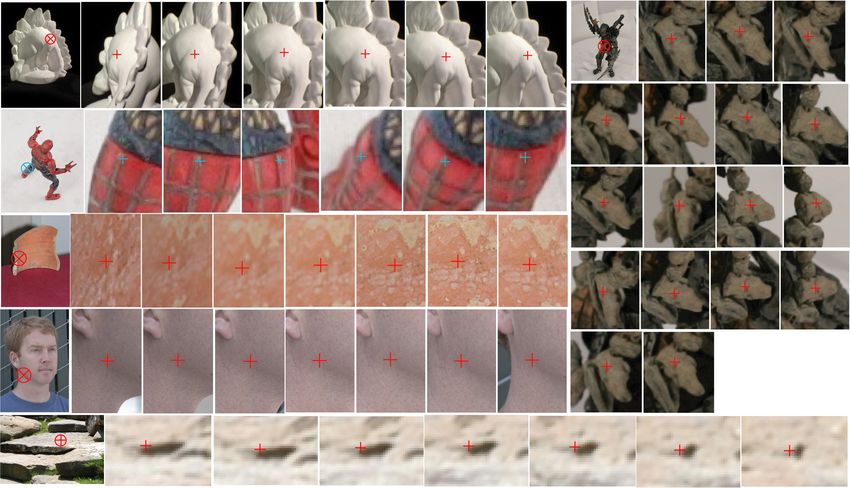
ure 9 shows matched images features for each dataset, while We have used a couple of different methods to qualita-
their colors represent the amounts of the associated final re- tively assess the accuracy of the estimated camera param-
projection errors: Red, green, and blue corresponds to two, eters. First, epipolar geometry has been used to check the
one, and zero pixels, respectively. Figure 10 shows the mean consistency between pairs of images (Fig. 11). More con-
and standard deviation of these reprojection errors at each cretely, for a pair of images, we draw pairs of epipolar lines
iteration of our algorithm for every dataset. The bottom-left in different colors to see if corresponding epipolar lines of
graph shows the number of 2D features matched and used to the same color pass through the same feature points in the7
Fig. 6 A set of matching 2D features is shown for each dataset. The proposed method is able to match features in many images even without
salient textures due to the use of surface geometry and visibility information estimated by the multi-view stereo algorithm.
400
Vase 450
Dino 350
Face 300
Spiderman 700
Predator Step
1800
350 400 300 600 1600
250
# of matches
300 350 1400
250 500
300 200 1200
250
250 200 400 1000
200 150
200 150 300 800
150
150 100 600
100 200
100 100 400
50 50 100
50 50 200
0 0 0 0 0 0
2 3 4 5 6 7 8 9 10 11 12 2 3 4 5 6 7 8 2 3 4 5 6 7 8 9 10 11 2 3 4 5 6 7 8 9 0 5 10 15 20 25 2 3 4 5 6 7
# of images in a match # of images in a match # of images in a match # of images in a match # of images in a match # of images in a match
Fig. 7 Histograms of the number of images in which features are matched by the proposed algorithm.
two images. Several images in the vase dataset contained 1974) or a hybrid model combining silhouette and texture
large errors before refinement (approximately six pixels in information (Furukawa and Ponce, 2006), (Hernández Este-
some places) because of the limited depth of field and an ban and Schmitt, 2004), (Sinha and Pollefeys, 2005), (Tran
exposure difference due to the use of a flash. The spider- and Davis, 2006). In turn, this requires a high degree of ge-
man and predator datasets also contain very large errors, up ometric consistency over the cameras, and provides a good
to seven (or possibly more) pixels for points far from the testing ground for our algorithm. We have used the EPVH
ground plane where the calibration chart is located. In each software of Franco and Boyer (Franco and Boyer, 2003)
case, the proposed method has been able to refine camera pa- to construct polyedral visual hulls in our experiments, and
rameters to sub-pixel level precision. Inconsistencies in the Fig. 12 shows that thin, intricate details such as the fingers
dino dataset introduced by the added noise have also been of spiderman and the blades of predator are successfully re-
corrected by our method despite its weak texture. covered with refined camera parameters, and completely lost
Next, we have tested the ability of our algorithm to re- otherwise.
cover camera parameters that are highly consistent across For dino and face, we have used PMVS to reconstruct a
widely separated views. We use the spiderman and preda- set of patches that are then converted into a 3D mesh model
tor datasets in this experiment (Fig. 12) since parts of these using the method described in (Kazhdan et al, 2006) (Fig. 12,
objects are as thin as a few pixels in many images. Recover- bottom right). The large artifacts at the neck and the chin of
ing such intricate structures normally requires exploiting sil- the shaded face reconstruction before refinement are mainly
houette information in the form of a visual hull (Baumgart, side effects of the use of visual hull constraints in PMVS8
Fig. 9 Matched image features are shown for each data set. The colors represent the associated reprojection errors computed after the last bundle
adjustment step. See text for more details.
Vase (SFM) Step (SFM) (patches are not reconstructed outside the visual hull (Fu-
2500 400
350 rukawa and Ponce, 2007)), exacerbated by the fact that the
2000
300 meshing method of (Kazhdan et al, 2006) extrapolates the
1500 250
200
surface in areas where data is not present. Ignoring these ar-
1000 150 tifacts, the difference in quality between the reconstructions
500
100 before and after refinement is still obvious in Fig. 12, near
50
the fins of the dinosaur, or the nose and mouth of the face
0 0
2 4 6 8
# of images in a match
10 12 2 3 4 5
# of images in a match
6 7 for example. In general, however, the accumulation of errors
due to geometric inconsistencies among widely separated
Fig. 8 Histograms of the number of images in which features are
cameras is not always visually recognizable in 3D models
matched with a standard SFC/SfM/BA software (Courchay, 2007) for
vase and step datasets. In comparison to the proposed algorithm whose reconstructed by multi-view stereo, because detailed local
results are presented in Fig. 7, features are matched in fewer images. reconstructions can be obtained from a set of close cameras,
and wide-baseline inconsistencies turn out as low-frequency
errors. In order to assess the effectiveness of our algorithm in
Mean reprojection errors [pixel]
reprojection errors [pixel]
handling this issue, we pick a pair of widely separated cam-
Standard deviation of
eras C1 and C2 , map a texture from one camera C 1 onto the
reconstructed model, render it as seen from C 2 , and compare
the rendered model with the input image associated with C 2 .
The two images should look the same (besides exposure dif-
ferences) when the camera parameters and the 3D model
# of iterations # of iterations are accurate. Figure 13 illustrates this on the vase and face
Za
datasets: Mesh models obtained again by combining PMVS
# of features matched
Vase Dino (Furukawa and Ponce, 2007) and the surface extraction algo-
rithm of (Kazhdan et al, 2006) are shown for both the initial
Face Spiderman and refined camera parameters. Although the reconstructed
Predator Step
vase models do not look very different, the amount of drift-
ing between rendered and input images is approximately six
pixels for initial camera parameters. Similarly, for the face
# of iterations
model, the reconstructed surfaces at the left cheek just be-
Fig. 10 The mean and standard deviation of reprojection errors in pixel side the nose look detailed and similar to each other, while
for each dataset at each iteration. The bottom-left graph shows the total
number of matched 2D features per iteration.
the rendered image is off by approximately six pixels as
well. In both cases, the error decreases to sub-pixel levels af-
ter refinement. Note that reducing low-frequency errors may
not necessarily improve the appearance of 3D models, but is9 Fig. 11 Epipolar lines are used to assess the improvements in camera parameters. A pair of epipolar lines of the same color must pass through the same feature points.
10

Fig. 12 Visual hull models are used to assess the accuracy of camera parameters for spiderman and predator. Intricate structures are reconstructed
only from the camera parameters refined by the proposed method. For dino and face, a set of patches reconstructed by PMVS and a 3D mesh
model extracted from these patches are used for the assessment. See text for more details.

essential in obtaining accuracy in applications where the ac-              Table 2 Running time in minutes of the three steps of the proposed
tual model geometry, and not just their overall appearance,                algorithm for the first iteration.
is important (e.g., engineering data analysis or high-fidelity                          vase    dino    face   spiderman      predator    step
surface modeling in the game and movie industries).                          PMVS        1.9    0.40    0.65      0.34           1.9       4.0
    Finally, the running time in minutes per iteration of the                Match       1.1    0.66    0.96      0.24           1.6      0.39
                                                                              BA        0.17    0.13    0.17      0.03          0.38       1.2
three steps (PMVS, feature matching, bundle adjustment) of
the proposed algorithm on a Dual Xeon 3.2GHz PC is given
in Table. 2. As shown by the table, the proposed algorithm                 on scaled-down input images is used to effectively estab-
is efficient and takes at most a few minutes per iteration to              lish feature correspondences. By taking into account the sur-
refine camera parameters. Note that the running time of typ-               face orientation and the visibility information estimated by
ical CBC systems is also in an order of a few minutes for                  a multi-view stereo system, the proposed method has been
these data sets. SFC/SFM/BA systems are more computa-                      able to match features in many views taken from quite dif-
tionally expensive, and in particular, a local implementation              ferent angles even when image textures are very weak. We
(Matlab) of a standard SFC/SFM/BA software takes several                   have performed three different ways to qualitatively assess
hours to calibrate the step data set with full resolution im-              the accuracy of refined camera calibration, which shows that
ages. As explained before, the proposed approach reduces                   the proposed method has successfully reduced calibration
such computational expenses for the step data set by first                 errors significantly. Future work will focus on the analysis of
running a SFC/SFM/BA system with scaled-down input im-                     remaining errors and influences of various factors that have
ages, which takes only a few minutes, then using the pro-                  been ignored in the current framework, such as the second
posed method to tighten up camera calibration.                             order effects in the camera projection model (distortions) or
                                                                           surface reflectance properties that are assumed to be Lam-
                                                                           bertian. The implementation of the proposed algorithm is
5 Conclusion                                                               publicly available at (Furukawa and Ponce, 2008b).

We have proposed a novel approach for camera calibration
                                                                           Acknowledgements This paper was supported in part by the National
where top-down information from rough camera parame-                       Science Foundation under grant IIS-0535152, the INRIA associated
ter estimates and the output of a multi-view stereo system                 team Thetys, and the Agence Nationale de la Recherch under grants
11
Fig. 13 Inconsistencies in widely separated cameras (accumulation errors) are often not recognizable from 3D mesh models reconstructed by a
MVS algorithm. For further assessments, we pick a pair of separated cameras shown in the middle row, texture-map the surface from the right
image, render it to the left, and compare the rendered model with the left image. The rendered and the input images look the same only if camera
parameters and the reconstructed model are accurate. The top and the bottom rows show rendered images and the reconstructed 3D mesh model
before and after the refinement, respectively. The amount of errors with the initial camera parameters (calibrated by SFM for vase and manual
feature correspondences for face) is roughly six pixels for both datasets, which are very large.
Hfimbr and Triangles. We thank S. Sullivan, A. Suter, and Industrial Furukawa Y, Ponce J (2008b) PBA. URL http://
Light and Magic for the face data set and support of this work. We also www-cvr.ai.uiuc.edu/∼yfurukaw/research/pba
thank Jerome Courchay for the SfM software, and Jean-Baptiste Houal
Furukawa Y, Ponce J (2008c) PMVS. URL http:
for the vase dataset.
//www-cvr.ai.uiuc.edu/∼yfurukaw/research/
pmvs/index.html
Hartley RI, Zisserman A (2004) Multiple View Geometry in
References Computer Vision. Cambridge University Press
Hernández Esteban C, Schmitt F (2004) Silhouette and
Baumgart B (1974) Geometric modeling for computer vi- stereo fusion for 3D object modeling. CVIU 96(3)
sion. PhD thesis, Stanford University Hernández Esteban C, Schmitt F, Cipolla R (2007) Silhou-
Bouguet JY (2008) Camera calibration toolbox for matlab. ette coherence for camera calibration under circular mo-
URL http://www.vision.caltech.edu/bouguetj/ tion. PAMI 29
calib doc Kazhdan M, Bolitho M, Hoppe H (2006) Poisson surface
Courchay J (2007) Auto-calibration á partir d’une séquence reconstruction. In: Symp. Geom. Proc.
d’images. MVA internship report Lavest JM, Viala M, Dhome M (1998) Do we really need an
DXO (2008) DxO Labs. DxO Optics Pro accurate calibration pattern to achieve a reliable camera
(http://www.dxo.com). URL http://www.dxo.com calibration? In: ECCV
Fischler M, Bolles R (1981) Random sample consensus: Lourakis M, Argyros A (2008) SBA: A generic sparse bun-
A paradigm for model fitting with applications to image dle adjustment C/C++ package based on the Levenberg-
analysis and automated cartography. CACM 24(6) Marquardt algorithm. URL http://www.ics.forth.
Franco JB, Boyer E (2003) Exact polyhedral visual hulls. In: gr/∼lourakis/sba/
BMVC Martinec D, Pajdla T (2007) Robust rotation and translation
Furukawa Y, Ponce J (2006) Carved visual hulls for image- estimation in multiview reconstruction. In: CVPR, pp 1–8
based modeling. In: ECCV, pp 564–577 Nister D (2004) An efficient solution to the five-point rela-
Furukawa Y, Ponce J (2007) Accurate, dense, and robust tive pose problem. PAMI 26(6)
multi-view stereopsis. In: CVPR Quan L (1995) Invariants of six points and projective recon-
Furukawa Y, Ponce J (2008a) Accurate camera calibration struction from three uncalibrated images. PAMI 17(1)
from multi-view stereo and bundle adjustment. In: CVPR12 Seitz SM, Curless B, Diebel J, Scharstein D, Szeliski R (2006) A comparison and evaluation of multi-view stereo reconstruction algorithms. CVPR Sinha S, Pollefeys M (2005) Multi-view reconstruction us- ing photo-consistency and exact silhouette constraints: A maximum-flow formulation. In: ICCV Tran S, Davis L (2006) 3d surface reconstruction using graph cuts with surface constraints. In: ECCV Triggs B, McLauchlan P, Hartley R, Fitzgibbon A (2000) Bundle adjustment – A modern synthesis. In: Triggs W, Zisserman A, Szeliski R (eds) Vision Algorithms: Theory and Practice, LNCS, Springer Verlag, pp 298–375 Triggs W (1997) Auto-calibration and the absolute quadric. In: CVPR Tsai R (1987) A versatile camera calibration technique for high-accuracy 3D machine vision metrology using off- the-shelf TV cameras. J Robot Autom 3(4) Uffenkamp V (1993) State of the art of high precision indus- trial photogrammetry. In: Third International Workshop on Accelerator Alignment, Annecy, France Wong KK, Cipolla R (2004) Reconstruction of sculpture from its profiles with unknown camera positions. IEEE Trans Im Proc
You can also read