Single-stage gradient-based stellarator coil design: stochastic optimization
←
→
Page content transcription
If your browser does not render page correctly, please read the page content below
Single-stage gradient-based stellarator coil design:
                                           stochastic optimization

                                                           Florian Wechsung1 , Andrew Giuliani1 , Matt Landreman2 ,
arXiv:2106.12137v1 [math.OC] 23 Jun 2021

                                                           Antoine Cerfon1 , Georg Stadler1
                                                           1 Courant Institute of Mathematical Sciences, New York University, New York,
                                                           USA
                                                           2 University of Maryland-College Park, Maryland, USA

                                                           E-mail: wechsung@nyu.edu, giuliani@cims.nyu.edu, mattland@umd.edu,
                                                           cerfon@cims.nyu.edu, stadler@cims.nyu.edu

                                                           24 June 2021

                                                           Abstract. We extend the single-stage stellarator coil design approach for quasi-
                                                           symmetry on axis from [Giuliani et al, 2020] to additionally take into account
                                                           coil manufacturing errors. By modeling coil errors independently from the coil
                                                           discretization, we have the flexibility to consider realistic forms of coil errors.
                                                           The corresponding stochastic optimization problems are formulated using a risk-
                                                           neutral approach and risk-averse approaches. We present an efficient, gradient-
                                                           based descent algorithm which relies on analytical derivatives to solve these
                                                           problems. In a comprehensive numerical study, we compare the coil designs
                                                           resulting from deterministic and risk-neutral stochastic optimization and find that
                                                           the risk-neutral formulation results in more robust configurations and reduces
                                                           the number of local minima of the optimization problem. We also compare
                                                           deterministic and risk-neutral approaches in terms of quasi-symmetry on and away
                                                           from the magnetic axis, and in terms of the confinement of particles released close
                                                           to the axis. Finally, we show that for the optimization problems we consider, a
                                                           risk-averse objective using the Conditional Value-at-Risk leads to results which
                                                           are similar to the risk-neutral objective.

                                           1. Introduction

                                           The design, manufacturing, and assembly of the primary coil system for stellarators
                                           are among the most technically challenging aspects of the construction of stellarators
                                           [Str+09; Nei+10; Kli+13], and represent a large fraction of the total construction
                                           cost. Some of these challenges are intrinsic to the nature of stellarators: non-
                                           axisymmetric coil systems are expected to be more complex than the axisymmetric
                                           coil systems of tokamaks [Str+09; Gat+18]. However, some of these challenges are
                                           directly linked to the design optimization process, and the optima which have been
                                           selected for construction. Specifically, the emphasis has historically been given to
                                           optimization metrics corresponding to plasma performance, and less attention was
                                           given to the engineering requirements and constraints to achieve such performance.
                                           Stellarator designs considered optimal from a physics point of view could only be
                                           realized with complex and expensive coil configurations. The difficulties encountered
                                           in the construction of large scale stellarators [Str+09; Nei+10; Kli+13] has recently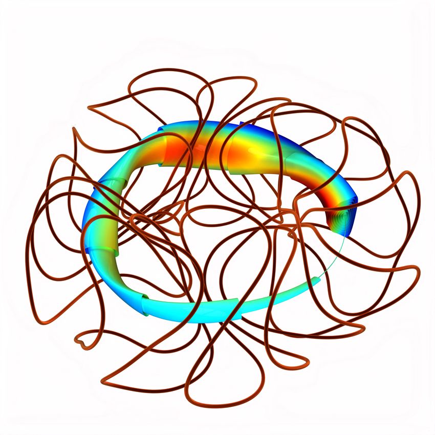
Stochastic Coil Design                                                                 2

triggered a renewed research effort toward the development of tools enabling the design
of simpler and more efficient coil systems that still lead to strong plasma performance
[LB16; Lan17; Hud+18; Pau+18; CPD21].
      Beside the engineering complexity of a given design, the lack of robustness of
the physics performance in the presence of coil manufacturing and assembly errors
is also a strong driver for the cost of a machine, since it requires tight tolerances
at every step of the manufacturing and assembly process. Both challenges are
related but not identical: a relatively simple coil system whose performance degrades
strongly with manufacturing and alignment errors may not be as desirable as a more
complex coil system with more robust performance. Work has therefore also been
lately devoted to the design of efficient numerical methods for the evaluation of the
sensitivity of error fields to coil perturbations [Zhu+18b; Zhu+19], and the sensitivity
of physical quantities to error fields [LP18; GLP21]. These methods can be included
in deterministic stellarator optimization codes, and serve to narrow the search to
configurations with lower sensitivity or with sensitivity with respect to perturbations
that are more easily controlled.
      A complementary approach to deal with the challenge of strong sensitivity and
tight tolerances is to account for errors during the optimization process, via stochastic
optimization. These errors may either be engineering errors or possibly errors due to
the limitations of the physics models used. In stochastic optimization, the objective
is a function both of the controls and of the random model errors and hence is
itself a random variable. This is precisely the approach we adopt in this article,
with the randomness corresponding to perturbations of the location and shape of
the coils. We observe that while stochastic optimization is not yet a widely applied
method for the design of magnetic confinement devices, it was used in the design
of the CNT stellarator [Kre+03; Ped+06]. CNT consists of four circular coils,
namely two interlocking (IL) coils and two poloidal field (PF) coils, and the CNT
optimization problem involves the angle between the IL coils, as well as the current
ratio between the IL and the PF coils. Coil errors involving tilts and shifts of these
coils were considered and the goal was to optimize the average volume with good flux
surfaces. More recently, for the problem of designing coils corresponding to a desired
plasma boundary, Lobsien et al. [Lob+20b; Lob+20a] demonstrated that stochastic
optimization leads to simpler and better performing coils.
      In this manuscript we present a stochastic version of the single-stage coil design
framework recently introduced in [Giu+20]. As the purpose of our work is mainly to
introduce a new paradigm for stochastic coil design optimization, the physics basis
for the design is simple: we consider a vacuum field, and optimize directly for a
target value of the rotational transform and for quasi-symmetry on the magnetic
axis. The main contribution of this work is a formulation that enables us to consider
more general and realistic coil perturbations than considered thus far, to implement
gradient based optimisation algorithms relying on analytic derivatives, and to compare
the performance of different forms of stochastic optimization.
      We find that both the stochastic and deterministic formulations result in different
designs depending on the initialization of the optimization algorithm, which indicates
the existence of multiple local minima. However, the variability of the designs
corresponding to the stochastic problem is substantially reduced as compared to the
designs obtained from the deterministic optimization problem. The coil systems we
obtain for different initial conditions are much more similar to one another when
using stochastic optimization than with deterministic optimization. We compare the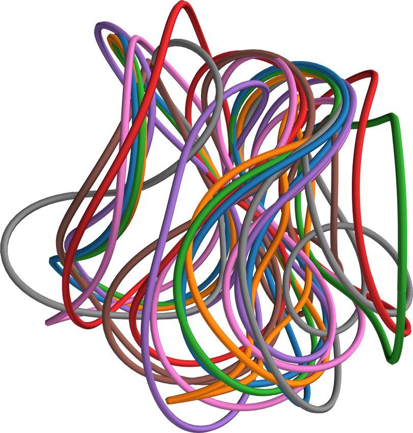
Stochastic Coil Design                                                                                 3

performance of the obtained configurations in the presence of coil errors by evaluating
the level of quasi symmetry near and away from the axis, the rotational transform
on axis as well as particle loss fraction. We observe that the configurations found by
stochastic optimization outperform those obtained from the deterministic formulation.
Furthermore, the different minima obtained from stochastic minimization all perform
very similarly, which suggests that the optimization algorithm does not get trapped in
poor local minima. For all these reasons, our work demonstrates the strong potential
of stochastic optimization for stellarator design, and motivates its application to more
detailed reactor design studies.
     The structure of the article is as follows. In Section 2, we present our
mathematical description of the coils, and explain how we model random coil
perturbations. In Section 3, we provide a brief summary of stochastic optimization,
with a description of several variants which are relevant to stellarator design. We
then review in Section 4 the direct coil design paradigm that we modify for stochastic
optimization, first introduced in [Giu+20]. We present our main numerical results in
Section 5, and summarize our work in Section 6, where we also suggest directions for
future work.

2. Modeling coil perturbations

2.1. Physical representation of coil perturbations
For this work, we make the common assumption in coil design that we can represent
the coils as current-carrying filaments, i.e., we neglect the non-zero thickness of the
coils, and simply model coils as curves in space. A coil is then described by a periodic
function Γ : [0, 2π) → R3 . A standard approach to discretizing such coils is given by
a truncated Fourier expansion, that is the j-th coordinate of the i-th coil Γ(i) is given
by
                                           ncoil
                                            p                         ncoil
                                                                       p
                    (i)          (i)                (i)                        (i)
                                           X                          X
                   Γj (θ)   =   cj,0   +           sj,l   sin(lθ) +           cj,l cos(lθ).           (1)
                                           l=1                        l=1
                                                                                              coils
We collect the degrees of freedom for coil i in the vector c(i) ∈ R3(2np +1) . This
approach is also used in the FOCUS code [Zhu+18c]. We note that this formulation
allows the coils to move freely in space, as compared to coil optimization codes that
restrict the coils to lie on the so-called winding surface. This latter approach is
employed in the ONSET [Dre99], COILOPT [SBH02], COILOPT++ [Gat+17] codes.
     A straightforward way of modelling errors is to perturb the vector containing
the degrees of freedom, c̃(i) = c(i) + ε where ε is a vector of independent random
variables. In the context of coil optimization, this approach has been used in [Lob+18;
Lob+20b; Lob+20a] which builds on ONSET and uses splines to represent coils. There
the spline anchor points were perturbed by independent, centered Gaussian random
variables with small variance. This approach does not require any modification of the
objective function implementation and hence a deterministic code can be extended
towards stochastic optimization with little effort.
     However, coil errors originate from the manufacturing process and are thus
independent of the coil description used in the design process. Thus, it is unlikely
that manufacturing errors satisfy stellarator symmetry [DH98], a property that most
optimization studies and coil design codes assume for simplicity [Dre+13; Zhu+18c;
Bad+19; Hen+19]. Hence, using the same parametrization for coil errors as used for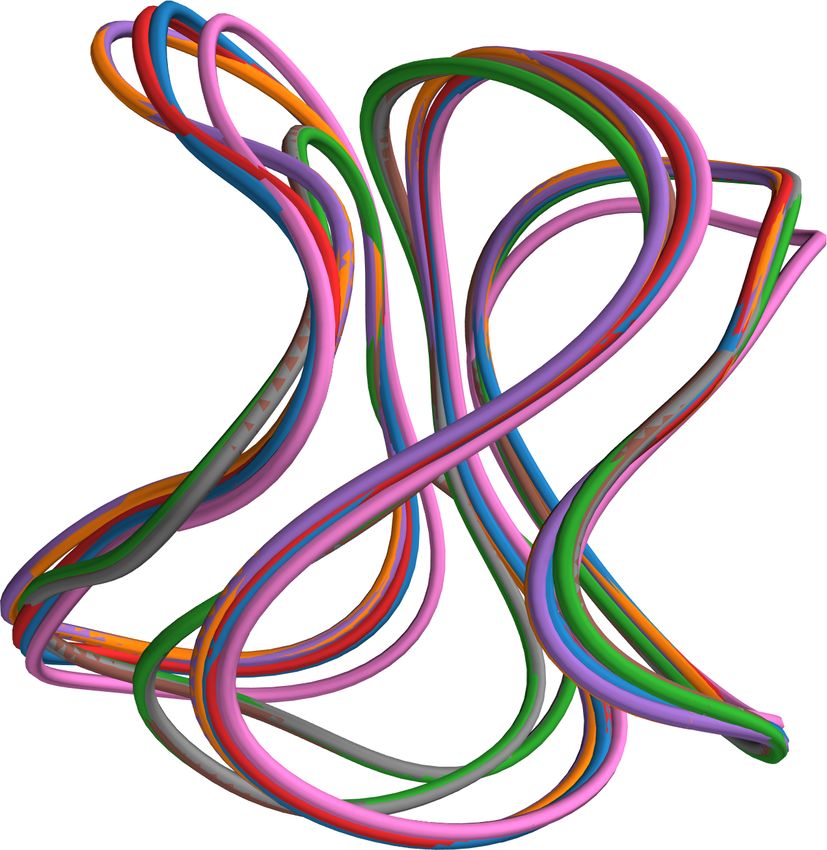
Stochastic Coil Design                                                                     4

the coils lacks generality, and may be unphysical. For instance, when Fourier modes
are used for coils and coil errors, these errors affect coils globally and repeat themselves
along the coils, with more repetitions with increasing Fourier mode numbers. Using
splines to describe the coil geometry as well as manufacturing errors has the advantage
of allowing the description of local manufacturing errors. However, if the number of
spline anchor points changes, the characteristics of the manufacturing error changes as
well. Thus, when the description of the coils and the errors is the same, changing the
coil discretization also means changing the type of errors considered and convergence
to a limit when refining the coil description is unclear.
     For this reason, we separate the discretization of the coils and the modelling of
perturbations by considering additive perturbations modelled by Gaussian processes
[RW06b]. To the best of our knowledge, this is a novel approach for stellarator coil
optimization applications. However, similar approaches have been used in other areas.
For instance, such an approach has been used in the context of airfoil optimization in
two dimensions [CC11; Wan+11; Liu+17].

2.2. Randomly perturbed coils via stochastic processes
We model the perturbations of the coil by random, periodic functions Ξ : [0, 2π) → R3 ,
and denote the perturbed coil by Γ̃(θ) = Γ(θ) + Ξ(θ). We choose to model the
components (Ξ1 , Ξ2 , Ξ3 ) of Ξ as centered Gaussian processes.
      We briefly recall the definition and some basic properties of Gaussian processes.
A random function Ξ is a centered Gaussian process if for any fixed set {θ1 , . . . , θn }
the random vector (Ξ(θ1 ), . . . , Ξ(θn )) follows a multi-variate normal distribution with
mean zero. The function C(θ, θ0 ) = Cov(Ξ(θ), Ξ(θ0 )) is referred to as the covariance
function. Sampling a Gaussian process at points {θ1 , . . . , θn } is then as straightforward
as drawing a Gaussian vector with mean zero and covariance matrix {C(θi , θj )}i,j .
      In this work, we make the common assumption that the covariance is stationary,
i.e., it is only a function of θ − θ0 . Thus, one can write C(θ, θ0 ) = k(θ − θ0 ) for some
function k. The regularity of the random functions Ξ is directly linked to the regularity
of k; in this work we consider a classical squared exponential covariance function,

                                                      d2

                                             2
                                   k(d) = σ exp − 2 ,                                     (2)
                                                      2l

which results in rather smooth perturbations. Here σ > 0 controls the overall
magnitude of the perturbations, and l > 0 is a measure for its length scale. For
our problem, we cannot use the covariance function k directly, because we need to
guarantee periodicity of Ξ. To address this minor difficulty, we rely on the fact that
any covariance function k can be made periodic on [0, 2π) by defining
                                       X
                               k̃(d) =    k(d + j2π),                              (3)
                                          j∈Z

see [SS02, (4.42)]. We thus use k̃ instead of k for our optimization studies. For
our construction of k̃, we truncate the sum (3) after just a few terms, since k has
exponential decay.
     Finally, since our optimization algorithms require the knowledge of derivatives,
an additional property of Gaussian processes is relevant to our work. By linearity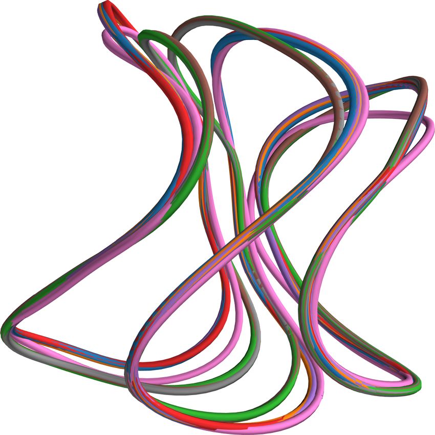
Stochastic Coil Design 5
(see [RW06a, §9.4], [Adl10, §2.2]) the derivatives of Ξ are also Gaussian and satisfy,
for θ, θ̄:
Cov(Ξ0 (θ), Ξ(θ̄)) = ∂θ C(θ, θ̄) = k̃ 0 (θ − θ̄)
Cov(Ξ(θ), Ξ0 (θ̄)) = ∂θ̄ C(θ, θ̄) = −k̃ 0 (θ − θ̄) (4)
0 0 00
Cov(Ξ (θ), Ξ (θ̄)) = ∂θ ∂θ̄ C(θ, θ̄) = −k̃ (θ − θ̄),
where the prime denotes derivative with respect to its argument. Thus, we can
draw samples {Ξ(θ1 ), . . . , Ξ(θn ), Ξ0 (θ1 ), . . . , Ξ0 (θn )} by drawing a Gaussian vector with
covariance matrix
0
k̃(θ1 − θ1 ) . . . k̃(θ1 − θn ) −k̃ 0 (θ1 − θ1 ) . . . −k̃ (θ1 − θn )
.. .. .. .. .. ..
. . . . . .
k̃(θn − θ1 ) . . . k̃(θn − θn ) −k̃ 0 (θn − θ1 ) . . . −k̃ 0 (θn − θn )
Σ= 0 . (5)
k̃ (θ1 − θ1 ) . . . k̃ 0 (θ1 − θn ) −k̃ 00 (θ1 − θ1 ) . . . −k̃ 00 (θ1 − θn )
.. .. .. .. .. ..
. .
. . . .
0 0 00 00
k̃ (θn − θ1 ) . . . k̃ (θn − θn ) −k̃ (θn − θ1 ) . . . −k̃ (θn − θn )
The standard approach to drawing such samples is to compute a matrix square root
Σ = LLT (e.g. via a Cholesky decomposition) and to draw a standard Gaussian vector
z. It is then straightforward to check that Cov(Lz) = Σ. We show several random
function draws from this Gaussian process as well as a perturbed coil in Figure 1.
1
σ = 0.05, l = 0.20
σ = 0.30, l = 0.20
σ = 0.30, l = 0.05
0.5
Perturbation
0
−0.5
−1
0 0.5 1 1.5 2 2.5 3 3.5 4 4.5 5 5.5 6
φ
Figure 1. Left: examples of periodic Gaussian processes for different parameter
choices σ and l in (2). Right: a coil perturbed with a Gaussian process sample
corresponding to σ = 0.1, l = 0.2. This large value of σ has been chosen for
illustration purposes. In our design process we choose smaller σ modeling realistic
manufacturing errors.
3. Stochastic and risk-averse optimization
In this Section, we briefly review the mathematical formulations of the different forms
of stochastic optimization one may favour, depending on the coil optimization design
goals and the level of risk one is willing to tolerate.
Let f ({Γ(i) }ni=1
c
, q) be some quantity of interest which one wants to minimize,
and which depends on the coil geometry {Γ(i) }ni=1 c
, as well as other quantities q ∈ Rnq
(e.g. coil currents). We define
g(({Γ(i) }ni=1
c
, q), {Ξ(i) }ni=1
c
) = f ({Γ(i) + Ξ(i) }ni=1
c
, q) (6)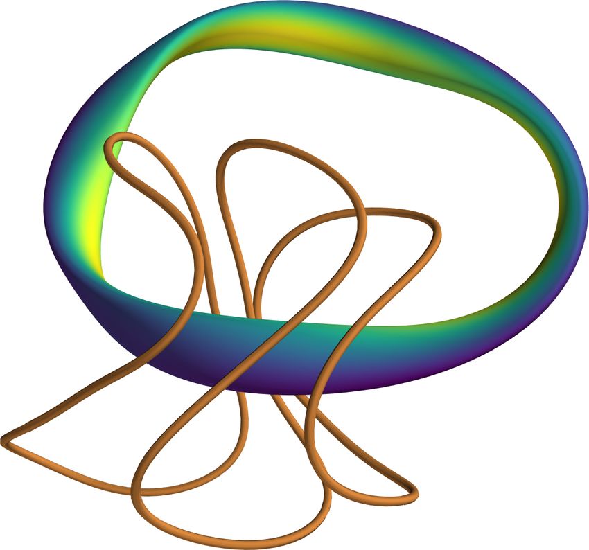
Stochastic Coil Design                                                                 6

For notational brevity we write x = ({Γ(i) }ni=1   c
                                                     , q) and ζ = {Ξ(i) }ni=1
                                                                           c
                                                                              , i.e., the
variables to be optimized are contained in x and the randomness is contained in
ζ. For fixed x, g(x, ζ) is now a random variable, which needs to be scalarized
in order to perform optimization. Risk-neutral, risk-averse, and robust stochastic
optimization formulations are all obtained by different ways of scalarising g(x, ζ),
and thus all take the distribution of manufacturing errors into account. While other
stochastic optimization formulations exist (e.g., [SDR09]), we only describe these three
below, since they are the most common formulations, and well suited to stellarator
optimization.
     Before we do so, we observe that the deterministic optimization problem of
minimizing f is equivalent to minimizing
                                      min g(x, 0),                                   (7)
                                          x

i.e., it is assumed that no coil error is present. This is the approach traditionally
taken in stellarator optimization, sometimes followed by perturbation tests at the
optimal design [Rum+04; Zhu+18c; Zhu+18a; Giu+20] to evaluate the sensitivity of
the objective with respect to coil errors. In contrast, the approaches discussed next
take the distribution of manufacturing errors into account during the optimization
process.

3.1. Types of optimization under uncertainty
3.1.1. Risk-neutral stochastic optimization Risk-neutral stochastic optimization
corresponds to the situation in which one wants to find a solution x that performs
optimally with respect to the mean of the realisations. We thus obtain the optimization
problem
                                   min E [g(x, ζ)] ,                                (8)
                                      x
where E [·] denotes expectation over the distribution of the perturbations ζ. In this
article, we will mainly focus on this approach, and thus sometimes simply refer to it as
stochastic optimization. However, for certain stellarator design problems and certain
objective functions, it can be desirable to explicitly avoid poor objective values for
some realizations of ζ. This can be achieved using risk-averse or robust formulations,
which we summarize next.

3.1.2. Risk-averse stochastic optimization: CVaR A measure that focuses on the tail
of the distribution is the conditional value-at-risk, or CVaR. The CVaR of a random
variable Z is defined as the expected value given that the random variable falls into
the α-quantile of its distribution, i.e.,
                          CVaRα [Z] = E Z|Z > CDF−1

                                                        Z (α) ,                   (9)
where CDFZ denotes the cumulative distribution function and α ∈ [0, 1]. The
difference between the risk-neutral formulation and CVaR is illustrated with an
example probability density function in Figure 2. This example highlights the fact
that the CVaR only depends on the tail of the distribution. One reason for the
popularity of CVaR over other risk-averse measures is its convexity as well as the
following equivalent formulation (cf. [RU00, Theorem 1])

                                              1           +

                      CVaRα [Z] = inf t +        E (Z − t)      ,             (10)
                                   t∈R      1−α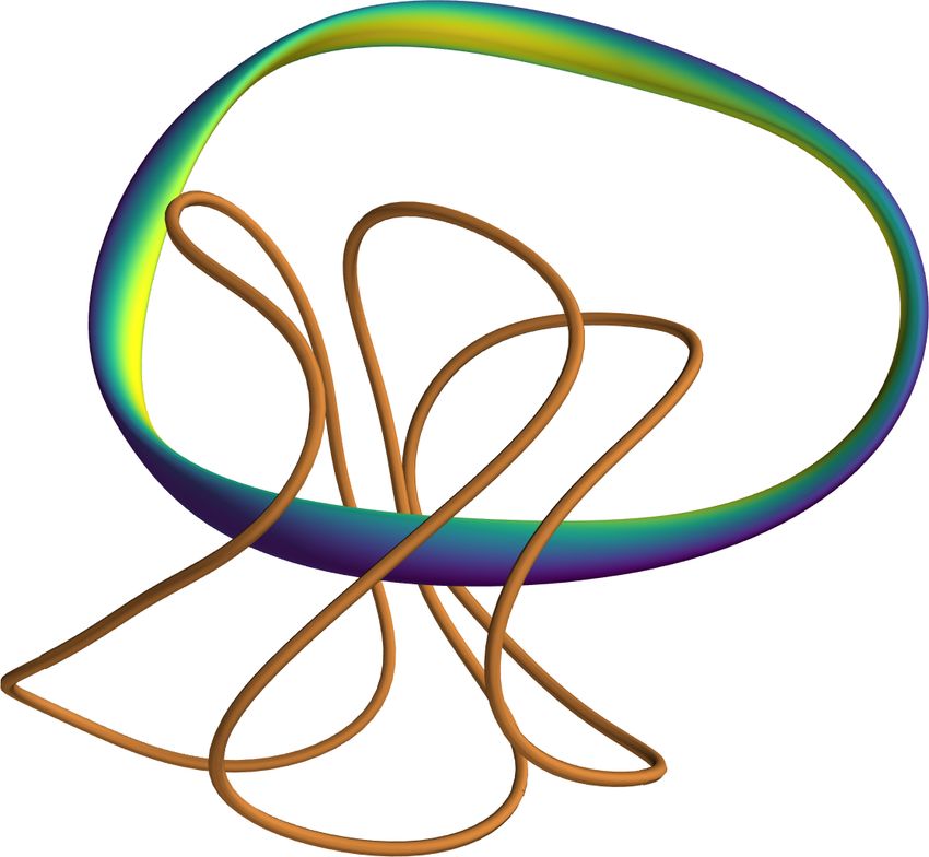
Stochastic Coil Design 7
where s+ := max(0, s), which is a convenient formulation for computational purposes.
To cope with the non-differentiable nature of the max-function, one relies in practice
on a smooth approximation hε : R → [0, ∞) with hε → ( · )+ as ε → 0. The specific
form of hε used in this work is
x
if x ≥ ε/2,
3
(x+ε/2)4
hε (x) = (x+ε/2)
ε2 − 2ε3 if − ε/2 < x < ε/2, (11)
0 otherwise.
We thus obtain the optimization problem
1
min t + E [hε (g(x, ζ) − t)] (12)
x,t 1−α
for a small ε. Risk-averse formulations based on CVaR are successfully used in the
insurance and finance industries and in engineering [RU00; KPU02; KS16] for instance.
0.8
Mean
0.6
pdf(X)
0.4 CDF−1
X (0.95)
0.2 CVaR0.95
0
0 0.5 1 1.5 2 2.5 3 3.5 4 4.5 5 5.5
X
Figure 2. Illustration of mean and CVaR with α = 0.95 for an example
distribution whose probability density function is shown in green.
3.1.3. Robust stochastic optimization To completely control the probability of poor
outcomes, one can optimize the worst possible scenario, i.e.,
min max g(x, ζ). (13)
x ζ
This formulation is typically combined with a model for randomness that results in
perturbations that are almost surely bounded. We will observe in Section 5 that the
difference between risk-neutral and risk-averse coil designs is minor for the stellarator
optimization problem we consider. Thus, we do not explore robust optimization
further in this article, as it can be viewed as an extreme version of risk-averse
optimization.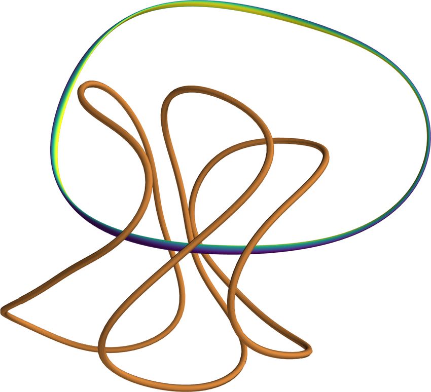
Stochastic Coil Design                                                               8

3.2. Sample average approximation
The expected value in (8) and (12) can typically not be computed analytically but
has to be approximated numerically. For that purpose, we use the sample average
approximation, i.e., we draw NMC independent realisations of ζk and approximate
                                                  NMC
                                             1    X
                           E [g(x, ζ)] ≈                g(x, ζk ),
                                            NMC
                                                  k=1
                                                                                  (14)
                                                  NMC
                                             1    X
                   E [hε (g(x, ζ) − t)] ≈               hε (g(x, ζk ) − t),
                                            NMC
                                                  k=1

for the risk-neutral and risk-averse formulation respectively. As NMC → ∞, the
                                                                                −1/2
random space approximation error is of the typical Monte Carlo order O(NMC ).
Since the samples ζk are kept fixed throughout the optimization, (14) results in a
deterministic optimization problem with NMC terms. Note that by linearity the sample
average approximation of the gradients is exactly equal to the gradient of the sample
average approximation.
     Our numerical tests in Section 5 focus on a comparison between deterministic,
risk-neutral and CVaR risk-averse stochastic designs. Moreover, we study the role of
the Monte Carlo sample size NMC for approximating the distribution.

4. Direct coil design for quasi-symmetry in vacuum fields

In [Giu+20] a new formulation was presented to directly design coils generating
vacuum magnetic fields which are quasi-symmetric to high accuracy in a region
close to the magnetic axis. We briefly recall the basic structure of the objective
that was developed there and then show the corresponding stochastic and risk-averse
formulations.
     Given a so-called expansion axis Γa and real parameter η̄ it was shown in [LS18;
LSP19] how to construct a magnetic field BQS that is quasi-symmetric near the axis
and how to compute its rotational transform ι. Calling Bcoils the magnetic fields
                           (i)
induced by the coils {Γc }, the approach of [Giu+20] is then to find coils so that
BQS ≈ Bcoils . Grouping the coefficients that describe the expansion axis and the real
parameter η in a vector a, and grouping the coefficients that describe the coils and
their currents in a vector c, the objective is given by
              Z                                    Z
   ˆ        1                            2       1
  J(c, a) =        kBcoils (c) − BQS (a)k dl +        k∇Bcoils (c) − ∇BQS (a)k2 dl
            2 Γa                                 2 Γa
                                !                                                  (15)
            1 (ι(a) − ι0,a )2
          +                       + Ra (a) + Rc (c),
            2        ι20,a

where ι0,a is a target rotational transform, and Ra and Rc contain various
regularizations for the expansion axis and coils respectively. The regularization terms
include penalty functions for the length of the axis and the length of the coils, the
curvature of the coils, and the distance between coils. In [Giu+20] it was shown that
this formulation leads to an efficient method to design from scratch coils producing
nearly quasi-symmetric vacuum magnetic configurations, and to improve the quasi-
symmetry properties of existing designs.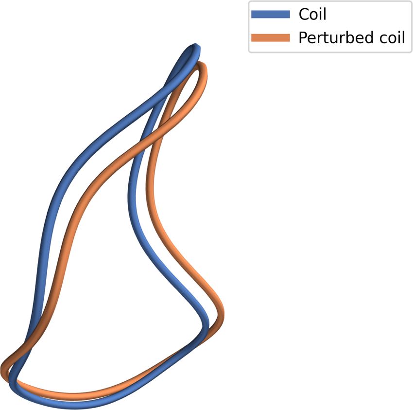
Stochastic Coil Design                                                                 9

      Random perturbations of the coils can be taken into account by considering the
objective
                 Z                                    Z
 ˆ a, ζ) = 1
 J(c,               kBcoils (c, ζ) − BQS (a)k2 dl +
                                                    1
                                                          k∇Bcoils (c, ζ) − ∇BQS (a)k2 dl
               2 Γa                                 2 Γa
               1 (ι − ι0,a )2

            +                   + Ra (a) + Rc (c),
               2     ι20,a
                                                                                     (16)
where Bcoils (c, ζ) corresponds to the magnetic field produced by the perturbed coils
{Γ(i) + Ξ(i) }. We emphasize here that the field BQS and the rotational transform
are independent from the random variable ζ, and hence we only have to recompute
Bcoils (c, ζ) and ∇Bcoils (c, ζ) for different samples ζ. We observe that as it is stated
here, the optimization problem can lead to numerical difficulties, because vanishing
derivatives of Γ(i) result in a non differentiable curve length objective, and because of
the large nullspace of the objective, which is partially due to the fact that different
parametrizations give the same physical curve. In order to address these numerical
difficulties, we add the following regularization term, in addition to the axis length,
coil length, coil curvature, and coil distance terms already included in [Giu+20],
                                   nc Z
                                   X                    0
                      Rarc (c) =                  (kΓ(i) (θ)k − t(i) )2 dθ,         (17)
                                   i=1   [0,2π)

                  i
                l
where t(i) = 2π     is the value that would correspond to a constant-arclength
parametrization of a circle with coil length l(i) .

5. Numerical results for NCSX-like example

5.1. Implementation and setup
We implement this optimization in the open source PyPlasmaOpt package available
under https://github.com/florianwechsung/PyPlasmaOpt. PyPlasmaOpt is a
Python library that relies on the geometric objects and the Biot Savart
implementation of the SIMSOPT stellarator optimization package http://github.
com/hiddenSymmetries/SIMSOPT. The implementation is parallelized across samples
using MPI, and the Biot Savart computation is accelerated using SIMD instructions
as well as OpenMP. A function and gradient evaluation of a typical configuration (18
coils, 120 quadrature points per coil) with 1024 samples takes less than half of a second
on a machine with two 24 Core Intel Xeon Platinum 8268 processors.
     To solve the optimization problems in (7), (8), and (12), we use the L-BFGS
implementation in SciPy [Vir+20]. For the smoothed risk-averse objective, we use
the risk-neutral minimizer as initial guess, then solve the optimization problem, then
reduce the smoothing parameter ε, and then solve the problem again, using the
previous solution as initial guess. This is repeated until ε = 10−5 .
     We study a configuration that is inspired by the National Compact stellarator
Experiment (NCSX). NCSX consists of three distinct modular coils, which results
in 18 coils after applying three fold rotational symmetry and stellarator symmetry.
We re-emphasize that while the design space only consists of coils that satisfy these
symmetries, the perturbations are not required to satisfy any form of symmetry. For
full details of the configuration we refer to [Giu+20, Section 6]. Finally, we note that
Stochastic Coil Design 10
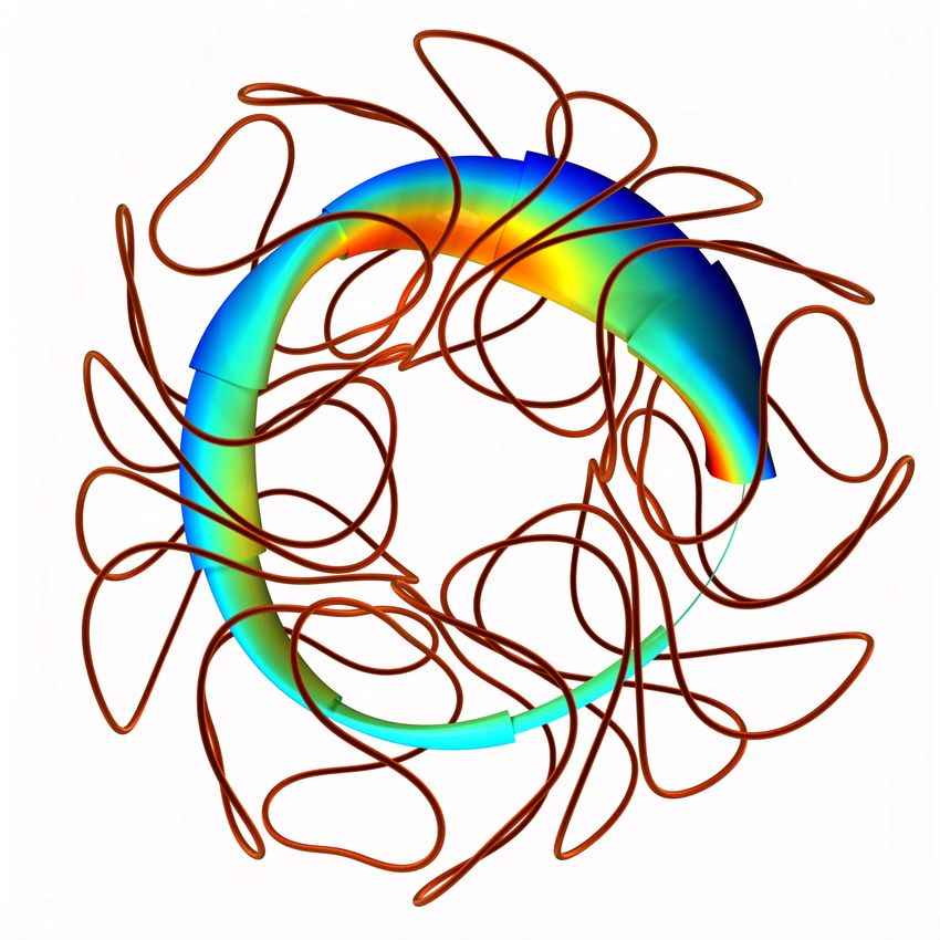
Figure 3. Two views of an optimal stellarator design computed using risk-neutral
stochastic optimization with NMC = 1024 samples with σ = 10−2 . We also show
a range of nested magnetic surfaces, with cool colors corresponding to low field
strength and warm colors corresponding to high field strength.
NCSX was designed for finite pressure equilibria, as opposed to the vacuum field that
we consider here, and that the additional planar coils of the NCSX design are ignored
in our calculations.
We study this problem in particular as the NCSX project was cancelled due to
increasing costs because of, among other reasons, the requirement of tight engineering
tolerances on the coils. To model the distribution of manufacturing errors, we choose a
length scale of l = 0.4π and a standard deviations of either σ = 10−2 or σ = 3 × 10⁻³
in the kernel (2) defining the Gaussian process. For each of the coils, these values
correspond to manufacturing errors of a few centimeters for σ = 10−2 and several
millimeters for σ = 3 × 10⁻³ .
When running the optimization algorithm with different initial guesses, we
observe that multiple local minima exist. For this reason, in the following sections we
usually show results for several different minima, that were obtained by starting the
optimizer from eight different initial guesses. These initial guesses were obtained by
randomly perturbing the Fourier coefficients describing the coils using independent
normal random variables with standard deviation of 0.01. One of the obtained
configurations together with a range of magnetic surfaces is shown in Figure 3. Next,
in Sections 5.2 and 5.3 we mainly focus on the role the number of samples NMC in
the sample average approximation (14) plays in approximating the distribution of
coil perturbations, and on the sensitivity of both the deterministic and the stochastic
minimizers on the initial guesses for the optimization algorithm.
5.2. Deterministic versus stochastic designs
Figure 4 shows minimizers that were obtained by solving the deterministic and the
stochastic optimization problem for eight different initial guesses. We clearly see that
for the deterministic problem there exists a large number of different minimizers thatStochastic Coil Design 11
are all distinct from each other. As coil errors (with σ = 10−2 ) are introduced and the
sample average approximation size NMC (see (14)) is increased, the number of distinct
minimizers that the algorithm finds is reduced and there is less variation between the
different coil designs. We note that the gradient was reduced by over 10 orders of
magnitude for all of these minimizers, so we can be confident that this result is not an
artifact of a possibly incomplete convergence of the algorithm. It is remarkable that
stochastic design formulations are significantly less prone to having multiple minima.
Intuitively, this can be understood by the fact that stochastic designs must perform
well on average for a distribution of manufacturing errors, which prevents overfitting
and also makes the objective locally convex in most directions around a minimizer. In
the following discussion, we find several additional advantages that designs computed
from a stochastic formulation have compared to designs based on a deterministic
formulation.
Figure 4. Optimal coil designs for the three independent coils. The designs
are obtained by using deterministic optimization (left), risk-neutral stochastic
optimization with NMC = 4 samples (middle) and with NMC = 1024 samples
(right) for eight different initial guesses (i.e., each panel shows 24 coil shapes).
Different colors correspond to different minimizers.
5.3. Out of sample distribution at the minimizer
As we only optimized the mean of the objective for a finite number of perturbations, we
have to check that this performance generalises to the full distribution of coil errors.
To do this we draw a large number (218 ) of new samples, which are different from
those used in the sample average approximation, and evaluate the objective at the
minimizer for each of the samples. In the context of statistics and machine learning,
this procedure is known as out-of-sample testing or cross validation. Figure 5 shows
the resulting distribution for minimizers obtained from deterministic and stochastic
optimization from eight different initial guesses. We see that the performance of the
minimizers of the deterministic optimization problem varies strongly on perturbed
coils. The minimizers found by stochastic optimization have lower objective value
on average and for most perturbations. In other words, the stochastic designs
perform significantly better than the deterministic designs. Additionally, different
minimizers obtained as a result of different initializations of the algorithm perform
vastly differently for the deterministic formulation, but very similarly for the stochastic
formulations, in particular when 1024 samples are used to estimate the expected value
in (14) for the stochastic formulation.Stochastic Coil Design 12
Objective distribution at minimizer
Deterministic
Stochastic (4 samples)
300 Stochastic (1024 samples)
200
100
0
0 0.5 1 1.5 2 2.5 3 3.5 4
Objective value ·10−2
Figure 5. Kernel density estimate for the distribution of the objective value
evaluated at minimizers obtained by running deterministic (red) and stochastic
optimization with NMC = 4 and NMC = 1024 samples used in the sample average
approximation (green and blue, respectively). Eight different initial guesses are
used for each optimization, leading to different minimizers and thus different
distributions. The distribution is approximated using 218 = 262, 144 independent
samples drawn from the error distribution.
5.4. Quasi-symmetry close to the axis
The objective is designed to ensure quasi-symmetry near the axis. To confirm that
this is achieved and to investigate the magnetic field away from the axis, we compute
magnetic flux surfaces S(ϕ, θ) parametrized by Boozer angles ϕ and θ. We recall
that a magnetic field is called quasi-axisymmetric if |B(S(ϕ, θ))| is a function of θ
only. Figure 6 shows three surfaces computed for the best configuration obtained
from stochastic optimization with NMC = 1024 samples. We can see that for the
surface closest to the axis, the field strength is indeed close to constant in ϕ. As we
move away from the axis, this property is gradually lost.Stochastic Coil Design 13
Magnetic field strength on surface Magnetic field strength on surface Magnetic field strength on surface
1.016 1.065 1.125
6 6 6
1.012 1.050 1.100
1.008 1.035 1.075
4 4 4 1.050
1.004 1.020
1.025
1.000 1.005
θ
θ
θ
1.000
0.996 0.990
2 2 2 0.975
0.992 0.975 0.950
0.988 0.960 0.925
0 0.984 0 0.945 0 0.900
0.00 0.25 0.50 0.75 1.00 0.00 0.25 0.50 0.75 1.00 0.00 0.25 0.50 0.75 1.00
φ φ φ
Figure 6. Top: Coils and magnetic surfaces in Boozer coordinates for the best
configuration obtained from stochastic optimization with NMC = 1024 samples.
Bottom: Strength of the magnetic field as a function of Boozer angles ϕ and θ
on the surfaces shown on the top. Perfect quasi-symmetry corresponds to the
magnetic field strength being independent of ϕ.
To quantify this statement, we decompose |B| into a quasi-symmetric and non-
quasi-symmetric part by defining
R
[0,2π)
kB(S(ϕ, θ))kk∂ϕ S × ∂θ Skdϕ
kBkQS (θ) = R
[0,2π)
k∂ϕ S × ∂θ Skdϕ
kBkNotQS (ϕ, θ) = kB(S(ϕ, θ))k − kBkQS (θ).
We then measure the norm of the non-quasi-symmetric part and report
RRS kBk2NotQS dS 1/2
RR
kBk2 dS
in Figure 7. Since we only enforce quasi-symmetry near the axis,
S QS
we expect this measure to be small for surfaces close to the axis, and to increase as
we move away from the axis.
We perform the stochastic optimization for σopt = 0.01 and σopt = 0.003. Quasi-
symmetry is then evaluated by drawing 20 new samples with standard deviation σs and
computing surfaces for the fields induced by the perturbed coils. The case of σs < σopt
can be viewed as the estimate for the perturbation size in the original optimization
being pessimistic, or be due to improvements in the manufacturing process between
design and construction of the coils. For comparison, we also compute surface
and non-quasi-symmetry for the minimizers obtained from deterministic optimization
(corresponding to σopt = 0). The results are displayed in Figure 7.
Overall we observe that the configurations have very little non-quasi-symmetric
contribution close to the axis, and that the non-quasi-symmetry then increases away
from axis. As can be expected, the difference between stochastic and deterministic
optimization is most significant for large coil perturbations (left plot, solid lines).
Keeping those same configurations, but reducing the perturbation magnitude in theStochastic Coil Design 14
newly drawn samples, we can see that the configurations obtained from both types of
optimization benefit from the added accuracy (left plot, dashed lines). Importantly,
the designs from stochastic optimization systematically perform better than those
from deterministic optimization.
For smaller perturbations (right) the behaviour remains qualitatively the same,
but the overall difference between stochastic and deterministic optimization is smaller.
This is expected, as in the limit of σopt → 0 the two optimization strategies become
identical.
Non quasi-symmetric part of B away from axis
10−2 10−2
kBNotQS kL2 /kBQS kL2
10−3 10−3
Deterministic (σopt = 0, σs = 0.01) Deterministic (σopt = 0, σs = 0.003)
Deterministic (σopt = 0, σs = 0.001) Deterministic (σopt = 0, σs = 0.0003)
Stochastic (σopt = 0.01, σs = 0.01) Stochastic (σopt = 0.003, σs = 0.003)
Stochastic (σopt = 0.01, σs = 0.001) Stochastic (σopt = 0.003, σs = 0.0003)
10−4 10−4
0 2 4 6 8 0 2 4 6 8
Surface area Surface area
Figure 7. Mean non-quasi-symmetry on a range of surfaces for eight different
minimizers obtained from deterministic and stochastic (NMC = 1024 samples)
optimization. Here we use the surface area as a label for the surfaces. Larger
surface areas correspond to surfaces farther from the axis.
5.5. Rotational transform on axis
The objective includes a penalty that targets a certain rotational transform on the
expansion axis. To investigate the impact of coil perturbation errors on rotational
transform, we draw 128 sets of perturbed coils, compute the magnetic axis for the
resulting magnetic fields, and then compute the rotational transform ι on axis. The
resulting distribution of ι is shown in Figure 8. As expected, for the perturbed coils the
target rotational transform is not achieved exactly. In agreement with our previous
results, we also observe that the different minimizers obtained from deterministic
optimization vary more than those obtained from stochastic optimization.Stochastic Coil Design 15
Distribution of rotational transform on axis
σ = 0.01
Deterministic
60 Stochastic (1024 samples)
Density
40
20
0
0.35 0.36 0.37 0.38 0.39 0.4 0.41 0.42 0.43 0.44 0.45
Rotational transform ι
σ = 0.003
Deterministic
200 Stochastic (1024 samples)
Density
100
0
0.35 0.36 0.37 0.38 0.39 0.4 0.41 0.42 0.43 0.44 0.45
Rotational transform ι
Figure 8. Distribution of the rotational transform ι on axis for each of the
eight minimizers found from deterministic and stochastic optimization. The
distribution is approximated using 128 independently drawn perturbed coil sets.
The dashed line indicated the target rotational transform.
5.6. Particle confinement
As a final measure of performance, we compute particle trajectories for perturbations
of the configurations obtained from deterministic and stochastic optimization. We
consider both 250eV protons and 1keV protons. For reference, we note that a 3.4keV
proton in our designs has approximately the same ratio of gyroradius to machine
size as an energetic alpha particle in the ARIES-CS reactor. We draw 10 perturbed
coil configurations for each minimizer obtained from deterministic and stochastic
optimization, as well as for the initial NCSX-like configuration. We then spawn 1120
protons with random pitch angle on random points along the magnetic axis and follow
them for 10ms, using the guiding center approximation [Boo80; Lit83; CB09] without
collisions. Particles are considered lost if they move more than 30cm away from the
axis. Figure 9 shows the average fraction of lost particles over time.
For both the lower energy protons and the higher energy protons considered
here, we observe that the configurations from stochastic optimization have better
confinement than the initial configuration and the configurations obtained from
deterministic optimization. In addition, we see again that the different minimizers
in the stochastic case all perform very similarly, whereas those from deterministic
optimization have highly varying performance. For the protons with lower energy,Stochastic Coil Design 16
Particle confinement for protons at 250eV
0.20
Fraction of particles lost
Initial
Deterministic
0.15 Stochastic
0.10
0.05
0.00
10−4 10−3 10−2
Time (s)
Particle confinement for protons at 1000eV
0.20
Fraction of particles lost
Initial
Deterministic
0.15 Stochastic
0.10
0.05
0.00
10−4 10−3 10−2
Time (s)
Figure 9. Particle losses over time for 250eV and 1000eV protons spawned
on axis, for perturbations of configurations obtained from stochastic and
deterministic optimization.
nearly all optimized configurations outperform the initial configuration. However, for
the protons with higher energy, this advantage is less clear. This suggests that quasi-
symmetry only close to the axis is in general insufficient to guarantee good particle
confinement, and motivates ongoing work on direct coil optimization enforcing quasi-
symmetry away from the axis.
5.7. Risk-neutral vs. risk-averse optimization
Finally, we compare the risk-neutral formulation (i.e. minimization of the expected
value) with a risk-averse objective for an error distribution with σ = 10−2 . We choose
α = 0.95 and minimize CVaRα (f ), meaning that we minimize the expected value of
the tail containing the 5% worst scenarios. In Figure 10 we show the out-of-sample
distribution of the objective evaluated at the minimizers. We can see that most of
the distribution for the risk-neutral objective is closer to zero, while the tail is slightly
thicker. However, the difference is insignificant. We attribute this to the quadratic
penalty form of our objective: since all objective values are positive and the objective
is squared, in order to control the mean large positive outliers have to be avoided.Stochastic Coil Design 17
Objective distribution at minimizer
400 Stochastic
CVaR0.9
300
200
100
0.4 0 0.6 0.8 1 1.2
0.2 0.4 0.6 0.8 1 1.2 1.4
Objective value
Objective value ·10−2
Figure 10. Distribution of objective values for designs computed using risk-
neutral stochastic formulation (blue) and CVaR risk-averse stochastic formulation
(pink). NMC = 1024 samples are used in the stochastic optimization, and the
distributions are computed using 262 144 independent samples. Slightly different
designs are obtained using eight initializations for the optimization.
6. Conclusion and future work
We have extended the direct stellarator design approach of [Giu+20] to include random
coil errors. We emphasize that our formulation uses separate discretizations for the
coils and their errors, which allows us to retain symmetries in the design space but
considers perturbations that do not satisfy them.
We then studied and compared deterministic, risk-neutral, and risk-averse
optimization for an NCSX-like example. We found that the deterministic problem
admits a large number of distinct minimizers which perform quite differently. Including
stochasticity reduces the number of different minimizers and results in minimizers that
all perform nearly identical in terms of both objective value, as well as quasi-symmetry
and rotational transform on and away from axis. Moving from a risk-neutral to a risk-
averse formulation does not result in significantly different minimizing designs in our
experiments: the tail of the distribution is reduced at the cost of somewhat worse
average performance. Finally, while we are able to achieve quasi-symmetry near the
axis, this property is lost away from axis. Current work is focused on including the
non-quasi-symmetry measure presented in Figure 7 on a range of surfaces to enforce
quasi-symmetry away from axis.
Acknowledgments
This work was supported by a grant from the Simons Foundation (560651). AG is
partially supported by a NSERC (Natural Sciences and Engineering Research Council
of Canada) postdoctoral fellowship. In addition, this work was supported in part
through the NYU IT High Performance Computing resources, services, and staff
expertise.REFERENCES 18
Code availability
The code used to generate the numerical results is openly available under
https://github.com/florianwechsung/PyPlasmaOpt/tree/fw/
paper-stochastic/examples/stochastic
References
Adler, Robert J. The Geometry of Random Fields. en. Society for Industrial and
Applied Mathematics, Jan. 2010. doi: 10.1137/1.9780898718980.
Bader, Aaron et al. “Stellarator equilibria with reactor relevant energetic particle
losses”. In: Journal of Plasma Physics 85.5 (2019), p. 905850508. doi: 10.1017/
S0022377819000680.
Boozer, Allen H. “Guiding center drift equations”. In: The Physics of Fluids 23.5
(1980), pp. 904–908. doi: 10.1063/1.863080. eprint: https://aip.scitation.
org/doi/pdf/10.1063/1.863080. url: https://aip.scitation.org/doi/
abs/10.1063/1.863080.
Carlton-Jones, Arthur, Elizabeth J Paul, and William Dorland. “Computing the shape
gradient of stellarator coil complexity with respect to the plasma boundary”. In:
Journal of Plasma Physics 87.2 (2021).
Cary, John R. and Alain J. Brizard. “Hamiltonian theory of guiding-center motion”.
In: Rev. Mod. Phys. 81 (2 May 2009), pp. 693–738. doi: 10.1103/RevModPhys.
81.693. url: https://link.aps.org/doi/10.1103/RevModPhys.81.693.
Chen, Shikui and Wei Chen. “A new level-set based approach to shape and topology
optimization under geometric uncertainty”. In: Structural and Multidisciplinary
Optimization 44.1 (July 2011), pp. 1–18. issn: 1615-147X, 1615-1488. doi: 10.
1007/s00158-011-0660-9.
Dewar, R.L. and S.R. Hudson. “Stellarator symmetry”. In: Physica D: Nonlinear
Phenomena 112.1 (1998). Proceedings of the Workshop on Time-Reversal
Symmetry in Dynamical Systems, pp. 275–280. issn: 0167-2789. doi: https :
//doi.org/10.1016/S0167-2789(97)00216-9.
Drevlak, M. et al. “ESTELL: A Quasi-Toroidally Symmetric Stellarator”. In:
Contributions to Plasma Physics 53.6 (2013), pp. 459–468. doi: 10.1002/ctpp.
201200055.
Drevlak, Michael. “Optimization of heterogenous magnet systems”. In: Proceedings of
the 12th International Stellarator Workshop. 1999.
Gates, D.A. et al. “Recent advances in stellarator optimization”. In: Nuclear Fusion
57.12 (Dec. 2017), p. 126064. doi: 10.1088/1741-4326/aa8ba0.
Gates, David A et al. “Stellarator research opportunities: a report of the National
Stellarator Coordinating Committee”. In: Journal of Fusion Energy 37.1 (2018),
pp. 51–94.
Geraldini, Alessandro, M. Landreman, and E. Paul. “An adjoint method for
determining the sensitivity of island size to magnetic field variations”. In: Journal
of Plasma Physics 87.3 (2021), p. 905870302. doi: 10.1017/S0022377821000428.
Giuliani, Andrew et al. “Single-stage gradient-based stellarator coil design:
Optimization for near-axis quasi-symmetry”. In: arXiv preprint arXiv:2010.02033
(2020).
Henneberg, S.A. et al. “Properties of a new quasi-axisymmetric configuration”. In:
Nuclear Fusion 59.2 (2019), p. 026014. doi: 10.1088/1741-4326/aaf604.REFERENCES 19
Hudson, S.R. et al. “Differentiating the shape of stellarator coils with respect to the
plasma boundary”. In: Physics Letters A 382.38 (2018), pp. 2732–2737. issn:
0375-9601. doi: https://doi.org/10.1016/j.physleta.2018.07.016.
Klinger, T. et al. “Towards assembly completion and preparation of experimental
campaigns of Wendelstein 7-X in the perspective of a path to a stellarator fusion
power plant”. In: Fusion Engineering and Design 88.6 (2013). Proceedings of the
27th Symposium On Fusion Technology (SOFT-27); Liège, Belgium, September
24-28, 2012, pp. 461–465. issn: 0920-3796. doi: https://doi.org/10.1016/j.
fusengdes.2013.02.153.
Kouri, D. P. and T. M. Surowiec. “Risk-Averse PDE-Constrained Optimization Using
the Conditional Value-At-Risk”. In: SIAM Journal on Optimization 26.1 (2016),
pp. 365–396. doi: 10.1137/140954556.
Kremer, JP et al. “The Status of the Design and Construction of the Columbia Non-
neutral Torus”. In: AIP Conference Proceedings. Vol. 692. Issue: 1. American
Institute of Physics, 2003, pp. 320–325.
Krokhmal, Pavlo, Jonas Palmquist, and Stanislav Uryasev. “Portfolio optimization
with conditional value-at-risk objective and constraints”. In: Journal of Risk 4
(2002), pp. 43–68.
Landreman, Matt. “An improved current potential method for fast computation of
stellarator coil shapes”. In: Nuclear Fusion 57.4 (Feb. 2017), p. 046003. doi:
10.1088/1741-4326/aa57d4.
Landreman, Matt and Allen H. Boozer. “Efficient magnetic fields for supporting
toroidal plasmas”. In: Physics of Plasmas 23.3 (2016), p. 032506. doi: 10.1063/
1.4943201.
Landreman, Matt and Elizabeth Paul. “Computing local sensitivity and tolerances
for stellarator physics properties using shape gradients”. In: Nuclear Fusion 58.7
(June 2018), p. 076023. doi: 10.1088/1741-4326/aac197. url: https://doi.
org/10.1088/1741-4326/aac197.
Landreman, Matt and Wrick Sengupta. “Direct construction of optimized stellarator
shapes. Part 1. Theory in cylindrical coordinates”. In: Journal of Plasma Physics
84.6 (2018), p. 905840616. doi: 10.1017/S0022377818001289.
Landreman, Matt, Wrick Sengupta, and Gabriel G. Plunk. “Direct construction
of optimized stellarator shapes. Part 2. Numerical quasisymmetric solutions”.
In: Journal of Plasma Physics 85.1 (2019), p. 905850103. doi: 10 . 1017 /
S0022377818001344.
Littlejohn, R. G. “Variational principles of guiding centre motion”. In: Journal of
Plasma Physics 29.1 (1983), pp. 111–125. doi: 10.1017/S002237780000060X.
Liu, Dishi et al. “Quantification of Airfoil Geometry-Induced Aerodynamic
Uncertainties—Comparison of Approaches”. In: SIAM/ASA Journal on Uncer-
tainty Quantification 5.1 (Jan. 2017), pp. 334–352. issn: 2166-2525. doi: 10 .
1137/15M1050239.
Lobsien, Jim-Felix et al. “Improved performance of stellarator coil design
optimization”. In: Journal of Plasma Physics 86.2 (Apr. 2020). doi: 10.1017/
S0022377820000227.
Lobsien, Jim-Felix et al. “Physics analysis of results of stochastic and classic stellarator
coil optimization”. In: Nuclear Fusion 60.4 (Apr. 2020). doi: 10.1088/1741-
4326/ab7211.REFERENCES 20
Lobsien, Jim-Felix et al. “Stellarator coil optimization towards higher engineering
tolerances”. In: Nuclear Fusion 58.10 (Oct. 2018). doi: 10.1088/1741- 4326/
aad431.
Neilson, G. H. et al. “Lessons Learned in Risk Management on NCSX”. In: IEEE
Transactions on Plasma Science 38.3 (2010), pp. 320–327.
Paul, E.J. et al. “An adjoint method for gradient-based optimization of stellarator coil
shapes”. In: Nuclear Fusion 58.7 (May 2018), p. 076015. doi: 10.1088/1741-
4326/aac1c7.
Pedersen, T. Sunn et al. “Experimental demonstration of a compact stellarator
magnetic trap using four circular coils”. In: Physics of Plasmas 13.1 (Jan. 2006).
issn: 1070-664X, 1089-7674. doi: 10.1063/1.2149313.
Rasmussen, Carl Edward and Christopher K. I. Williams. Gaussian processes for
machine learning. Adaptive computation and machine learning. Cambridge, Mass:
MIT Press, 2006.
Rasmussen, CE. and CKI. Williams. Gaussian Processes for Machine Learning.
Adaptive Computation and Machine Learning. Cambridge, MA, USA: MIT Press,
Jan. 2006, p. 248.
Rockafellar, R. Tyrrell and Stanislav Uryasev. “Optimization of conditional value-at-
risk”. en. In: The Journal of Risk 2.3 (2000), pp. 21–41. issn: 14651211. doi:
10.21314/JOR.2000.038.
Rummel, T. et al. “Accuracy of the Construction of the Superconducting Coils for
WENDELSTEIN 7-X”. en. In: IEEE Transactions on Appiled Superconductivity
14.2 (June 2004), pp. 1394–1398. issn: 1051-8223. doi: 10.1109/TASC.2004.
830584.
Schölkopf, Bernhard and Alexander J. Smola. Learning with kernels: support vector
machines, regularization, optimization, and beyond. Adaptive computation and
machine learning. Cambridge, Mass: MIT Press, 2002.
Shapiro, Alexander, Darinka Dentcheva, and Andrezj Ruszczynski. Lectures on
Stochastic Programming: Modeling and Theory. Society for Industrial and Applied
Mathematics, 2009.
Strickler, Dennis J., Lee A. Berry, and Steven P. Hirshman. “Designing Coils for
Compact Stellarators”. In: Fusion Science and Technology 41.2 (Mar. 2002),
pp. 107–115. doi: 10.13182/FST02-A206.
Strykowsky, R. L. et al. “Engineering cost schedule lessons learned on NCSX”. In:
2009 23rd IEEE/NPSS Symposium on Fusion Engineering. 2009, pp. 1–4.
Virtanen, Pauli et al. “SciPy 1.0: fundamental algorithms for scientific computing in
Python”. In: Nature Methods 17.3 (2020), pp. 261–272.
Wang, Qiqi et al. “Conditional sampling and experiment design for quantifying
manufacturing error of transonic airfoil”. In: 49th AIAA Aerospace Sciences
Meeting including the New Horizons Forum and Aerospace Exposition. Orlando,
Florida: American Institute of Aeronautics and Astronautics, Jan. 2011. isbn:
978-1-60086-950-1. doi: 10.2514/6.2011-658.
Zhu, Caoxiang et al. “Designing stellarator coils by a modified Newton method using
FOCUS”. In: Plasma Physics and Controlled Fusion 60.6 (Apr. 2018), p. 065008.
doi: 10.1088/1361-6587/aab8c2.
Zhu, Caoxiang et al. “Hessian matrix approach for determining error field sensitivity
to coil deviations”. In: Plasma Physics and Controlled Fusion 60.5 (Apr. 2018),
p. 054016. doi: 10.1088/1361-6587/aab6cb.REFERENCES 21
Zhu, Caoxiang et al. “Identification of important error fields in stellarators using the
Hessian matrix method”. In: Nuclear Fusion 59.12 (Sept. 2019), p. 126007. doi:
10.1088/1741-4326/ab3a7c.
Zhu, Caoxiang et al. “New method to design stellarator coils without the winding
surface”. In: Nuclear Fusion 58.1 (Jan. 2018), p. 016008. issn: 0029-5515, 1741-
4326. doi: 10.1088/1741-4326/aa8e0a.You can also read