MIST Multiple Instance Spatial Transformer Networks
←
→
Page content transcription
If your browser does not render page correctly, please read the page content below
MIST
                                              Multiple Instance Spatial Transformer Networks

                                                     Baptiste Angles                    Simon Kornblith                 Shahram Izadi
                                            University of Victoria / Google Inc.        Google Research                   Google Inc.
                                                   bangles@uvic.ca                  skornblith@google.com            shahrami@google.com
arXiv:1811.10725v3 [cs.CV] 1 Jun 2019

                                                            Andrea Tagliasacchi                              Kwang Moo Yi
                                                             Google Research                               University of Victoria
                                                        atagliasacchi@google.com                              kyi@uvic.ca

                                                                                       Abstract
                                                  We propose a deep network that can be trained to tackle image reconstruction and
                                                  classification problems that involve detection of multiple object instances, without
                                                  any supervision regarding their whereabouts. The network learns to extract the most
                                                  significant K patches, and feeds these patches to a task-specific network — e.g.,
                                                  auto-encoder or classifier — to solve a domain specific problem. The challenge
                                                  in training such a network is the non-differentiable top-K selection process. To
                                                  address this issue, we lift the training optimization problem by treating the result of
                                                  top-K selection as a slack variable, resulting in a simple, yet effective, multi-stage
                                                  training. Our method is able to learn to detect recurring structures in the training
                                                  dataset by learning to reconstruct images. It can also learn to localize structures
                                                  when only knowledge on the occurrence of the object is provided, and in doing so
                                                  it outperforms the state-of-the-art.

                                        1     Introduction
                                        The ability to find and process multiple instances of characteristic entities in a scene is core to many
                                        computer vision applications, including object detection [14, 28, 29], pedestrian detection [6, 31, 44],
                                        and keypoint localization [2, 22]. In traditional vision pipelines, a common approach to localizing
                                        entities is to select the top-K responses in a heatmap and use their locations [2, 8, 22]. However, this
                                        type of approach does not provide a gradient with respect to the heatmap, and thus it cannot be directly
                                        integrated into neural network-based computer vision systems. To overcome this challenge, previous
                                        work proposed to use grids [5, 14, 27] to simplify the formulation by isolating each instance [42],
                                        or to optimize over multiple branches [26]. While effective, these approaches require additional
                                        supervision to localize instances, and do not generalize well outside the application domain for which
                                        they were designed. Other formulations, such as sequential attention [1, 7, 12] and channel-wise
                                        approaches [46] are problematic to apply when the number of instances of the same object is large.
                                        Here, we introduce a novel way to approach this problem, which we term Multiple Instance Spatial
                                        Transformer, or MIST for brevity. As illustrated in Figure 1 for the image synthesis task, given an
                                        image, we first compute a heatmap via a deep network whose local maxima correspond to locations
                                        of interest. From this heatmap, we gather the parameters of the top-K local maxima, and then extract
                                        the corresponding collection of image patches via an image sampling process. We process each patch
                                        independently with a task-specific network, and aggregate the network’s output across patches.
                                        Training a pipeline that includes a non-differentiable selection/gather operation is non-trivial. To solve
                                        this problem we propose to lift the problem to a higher dimensional one by treating the parameters

                                        Preprint. Under review.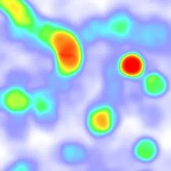
input                detector               heatmap                                      keypoints

                                                                          top-k

      forward pass
      backpropagation
      no gradient

                                           optimal heatmap

    loss                    task network                                           encoder
                                                           latent space

Figure 1: The MIST architecture – A network Hη estimates locations and scales of patches encoded
in a heatmap h. Patches are then extracted via a sampler S, and then fed to a task-specific network
Tτ . In this example, the specific task is to re-synthesize the image as a super-position of (unknown
and locally supported) basis functions.

defining the interest points as slack variables, and introduce a hard constraint that they must correspond
to the output that the heatmap network gives. This constraint is realized by introducing an auxiliary
function that creates a heatmap given a set of interest point parameters. We then solve for the relaxed
version of this problem, where the hard constraint is turned into a soft one, and the slack variables
are also optimized within the training process. Critically, our training strategy allows the network
to incorporate both non-maximum suppression and top-K selection. We evaluate the performance
of our approach for 1 the problem of recovering the basis functions that created a given texture,
 2 classification of handwritten digits in cluttered scenes, and 3 recognition of house numbers in
real-world environments. In summary, in this paper we:

 • introduce the MIST framework for weakly-supervised multi-instance visual learning;
 • propose an end-to-end training method that allows the use of top-K selection;
 • show that our framework can reconstruct images as parts, as well as detect/classify
   instances without any location supervision.

2   Related work

Attention models and the use of localized information have been actively investigated in the literature.
Some examples include discriminative tasks such as fine-grained classification [34] and pedestrian
detection [44], and generative ones such as image synthesis from natural language [19]. We now
discuss a selection of representative works, and classify them according to how they deal with multiple
instances.
Grid-based methods. Since the introduction of Region Proposal Networks (RPN) [29], grid-based
strategies have been used for dense image captioning [20], instance segmentation [14], keypoint
detection [10], multi-instance object detection [28]. Recent improvements to RPNs attempt to
learn the concept of a generic object covering multiple classes [32], and to model multi-scale
information [4]. The multiple transformation corresponding to separate instances can also be densely
regressed via Instance Spatial Transformers [41], which removes the need to identify discrete instance
early in the network. However, all these methods are fully supervised, requiring both class labels and
object locations for training.
Heatmap-based methods. Heatmap-based methods have recently gained interest to detect fea-
tures [5, 26, 42], find landmarks [23, 46], and regress human body keypoint [25, 38]. While it is
possible to output a separate heatmap per class [38, 46], most heatmap-based approaches do not

                                                    2
distinguish between instances. Yi et al. [42] re-formulates the problem based on each instance, but in
doing so it introduces a non-ideal difference between training and testing regimes. Grids can also be
used in combination with heatmaps [5], but this results in an unrealistic underlying assumption of
uniformly distributed detections in the image. Overall, heatmap-based methods excel when the “final”
task of the network is generate a heatmap [23], but are problematic to use as an intermediate layer in
the presence of multiple instances.
Sequential inference methods. Another way to approach multi-instance problems is to attend to
one instance at a time in a sequential way. Training neural network-based models with sequential
attention is challenging, but approaches employing policy gradient [1] and differentiable attention
mechanisms [7, 12] have achieved some success for images comprising small numbers of instances.
However, RNNs often struggle to generalize to sequences longer than the ones encountered during
training, and while recent results on inductive reasoning are promising [13], their performance does
not scale well when the number of instances is large.
Knowledge transfer. To overcome the acquisition cost of labelled training data, one can transfer
knowledge from labeled to unlabeled dataset. For example, Inoue et al. [16] train on a single instance
dataset, and then attempt to generalize to multi-instance domains, while Uijlings et al. [39] attempts
to also transfer a multi-class proposal generator to the new domain. While knowledge transfer can be
effective, it is highly desirable to devise unsupervised methods such as ours that do not depend on an
additional dataset.
Weakly supervised methods. To further reduce the labeling effort, weakly supervised methods
have also been proposed. Wan et al. [40] learns how to detect multiple instances of a single object
via region proposals and ROI pooling, while Tang et al. [36] proposes to use a hierarchical setup to
refine their estimates. Gao et al. [9] provides an additional supervision by specifying the number of
instances in each class, while Zhang et al. [45] localizes objects by looking at the network activation
maps [30, 47]. However, all these method still rely on region proposals from an existing method, or
define them via a hand-tuned process.
3 MIST framework
A prototypical MIST architecture is composed of two trainable components: 1 the first module
receives an image as input and extracts a collection of patches, at image locations and scales that are
computed by a trainable heatmap network Hη with weights η; see Section 3.1. 2 the second module
processes each extracted patch with a task-specific network Tτ whose weights τ are shared across
patches, and further manipulates these signals to express a task-specific loss Ltask ; see Section 3.2.
The two modules are connected through non-maximum suppression on the scale-space heatmap
output of Hη , followed by a top-K selection process to extract the parameters defining the patches,
which we denote as EK . We then sample patches at these locations through bilinear sampling S and
feed them the second module.
The defining characteristic of the MIST architecture is that they are quasi-unsupervised: the only
strictly required supervision is the number K of patches to extract. The training of the MIST
architecture is summarized by the optimization:
argmin Ltask (Tτ (S(EK (Hη (I))))) (1)
τ,η
where τ, η are the network trainable parameters. In this section, we describe the forward pass through
the MIST architecture. Because the patch extractor EK is non-differentiable, optimizing this objective
presents additional challenges, which we address in Section 4.
3.1 Patch extraction
We extract a set of K (square) patches that correspond to “important” locations in the image – where
importance is a direct consequence of Ltask . The localization of such patches can be computed by
regressing a 2D heatmap whose top-K peaks correspond to the patch centers. However, as we do not
assume these patches to be equal in size, we regress to a collection of heatmaps at different scales.
To limit the number of necessary scales, we use a discrete scale space with S scales, and resolve
intermediate scales via weighted interpolation.
3Multiscale heatmap network – Hη . Our multiscale heatmap network is inspired by LF-Net [26].
We employ a fully convolutional network with (shared) weights η at multiple scales, indexed by
s = 1 . . . S, on the input image I. The weights η across scales are shared so that the network cannot
implicitly favor a particular scale. To do so, we first downsample the image to each scale producing Is ,
execute the network Hη on it, and finally upsample to the original resolution. This process generates
a multiscale heatmap tensor h = {hs } of size H × W × S where hs = Hη (Is ), and H is the height
of the image and W is the width. For the convolutional network we use 4 ResNet blocks [15], where
each block is composed of two 3 × 3 convolutions with 32 channels and relu activations without any
downsampling. We then perform a local spatial softmax operator [26] with spatial extent of 15 × 15
to sharpen the responses. Then we further relate the scores across different scales by performing
a “softmax pooling” operation over scale. Specifically, if we denote the heatmap tensor after local
spatial softmax as h̃ = {h̃s }, since after the local spatial softmax Hη (Is ) is already an “exponentiated”
signal, we do a weighted normalization without an exponential, i.e. h0 = s h̃s (h̃s / s0 (h̃s0 + )),
P P
where = 10−6 is added to prevent division by zero.
Top-K patch selection – EK . To extract the top K elements, we perform an addition cleanup through
an actual non-maximum suppression. We then find the spatial locations of the top K elements of
this heatmap h̄s , denoting the spatial location of the k th element as (xk , yk ), which now reflect local
maxima. For each location, we compute the corresponding scale by weighted first Porder moments [35]
where the weights are the responses in the corresponding heatmaps, i.e. sk = s h0s (xk , yk )s.
Our extraction process uses a single heatmap for all instances that we extract. In contrast, existing
heatmap-based methods [7, 46] typically rely on heatmaps dedicated to each instance, which is
problematic when an image contains two instances of the same class. Conversely, we restrict the
role of the heatmap network Hη to find the “important” areas in a given image, without having to
distinguishing between classes, hence simplifying learning.
Patch resampling – S. As a patch is uniquely parameterized its location and scale xk = (xk , yk , sk ),
we can then proceed to resample its corresponding tensor via bilinear interpolation [17, 18]
as {Pk } = S (I, {xk }).
3.2 Task-specific networks
We now introduce two applications of the MIST framework. We use the same heatmap network and
patch extractor for both applications, but the task-specific network and loss differ. We provide further
details regarding the task-specific network architectures in Section B of the supplementary material.
Image reconstruction / auto-encoding. As illustrated in Fig. 1, for image reconstruction we append
our patch extraction network with a shared auto-encoder for each extracted patch. We can then
train this network to reconstruct the original image by inverting the patch extraction process and
minimizing the mean squared error between the input and the reconstructed image. Overall, the
network is designed to jointly model and localize repeating structures in the input signal. Specifically,
we introduce the generalized inverse sampling operation S −1 (Pi , xi ), which starts with an image
of all zeros, and places the patch Pi at xi . We then sum all the images together to obtain the
reconstructed image, optimizing the task loss
2
Ltask = kI − S −1 (Pi , xi ) k2 .
X
(2)
i
Multiple instance classification. By appending a classification network to the patch extraction
module, we can also perform multiple instance learning. For each extracted patch Pk we apply a
shared classifier network to output ŷk ∈ RC , where C is the number of classes. In turn, these are
then converted into probability estimates by the transformation p̂k = softmax(ŷk ). With yl being
the one-hot ground-truth labels of instance l, we define the multi-instance classification loss as
L K 2
1X 1 X
Ltask = yl , p̂k , (3)
L K
l=1 k=1 2
where L is the number of instances in the image. In our early experiments we tried cross entropy
in place of `2 , but it performed worse. Note here that we do not provide supervision about the
localization of instances, yet the detector network will automatically learn how to localize the content
with minimal supervision (i.e. the number of instances).
4Algorithm 1 Multi-stage optimization for MISTs
Require: K : number of patches to extract, Ltask : task specific loss, I : input image, η : parameters
of the heatmap network, τ : parameters of the task network.
1: function T RAIN MIST(I, Ltask )
2: for each training batch do
3: τ ← Optimize Tτ with Ltask
4: {x∗k } ← Optimize {xk } with Ltask
−1
5: h̄ ← EK ({x∗k })
6: η ← Optimize Hη with Llift
7: end for
8: end function
4 Training MISTs
The patch selector EK identifies the locations of the top-K local maxima of a heatmap, which is
not a differentiable operation. Although it is possible to smoothly relax this operation in the K = 1
case [42] (i.e. argmax), it is unclear how to generalize this approach to compute locations of multiple
distinct local maxima. We thus propose an alternative approach to training our model, using a
multi-stage optimization process. Empirically, this optimization process converges smoothly, as we
show in Section C of the supplementary material.
Differentiable top-K via lifting. The introduction of auxiliary variables (i.e. lifting) to simplify the
structure of an optimization problem has proven effective in a range of domains ranging from non-
rigid registration [37], to efficient deformation models [33], and robust optimization [43]. To simplify
our training optimization, we start by decoupling the heatmap tensor from the optimization (1) by
introducing the corresponding auxiliary variables h̄, as well as the patch parameterization variables
{xk } that are extracted by the top-K extractor:
argmin Ltask (Tτ (S({xk }))) s.t. {xk } = EK (h̄), h̄ = Hη (I) (4)
η,τ,h̄,{xk }
We then relax (4) to a least-squares penalty:
argmin Ltask (Tτ (S({xk }))) + kh̄ − Hη (I)k22 s.t. {xk } = EK (h̄) (5)
η,τ,h̄,{xk }
and finally approach it by alternating optimization:
argmin Ltask (Tτ (S({xk }))) (6)
τ,{xk }
argmin kh̄ − Hη (I)k22 (7)
η
−1
where h̄ has been dropped as it is not a free parameter: it can be computed as h̄ = EK ({xk }) after
the {xk } have been optimized by (6), and as h̄ = Hη (I) after η have been optimized by (7). To
accelerate training, we further split (6) into two stages, and alternate between optimizing τ and {xk }.
The summary for the three stage optimization procedure is outlined in Algorithm 1: 1 we optimize
the parameters τ with the loss Ltask ; 2 we then fix τ , and refine the positions of the patches {xk }
with Ltask . 3 with the optimized patch positions {x∗k }, we invert the top-K operation by creating a
target heatmap h̄, and optimize the parameters η of our heatmap network H using squared `2 distance
between the two heatmaps, Llift = kh̄ − Hη (I)k22 . Notice that we are not introducing any additional
supervision signal that is tangent to the given task.
−1
Generating the target heatmap – EK ({xk }). For creating the target heatmap h̄, we create a
tensor that has zeros everywhere except for the positions corresponding to the optimized positions.
However, as the optimized patch parameters are no longer integer values, we need to quantize them
with care. For the spatial locations we simply round to the nearest pixel, which at most creates a
quantization error of half a pixel, which does not cause problems in practice. For scale however,
simple nearest-neighbor assignment causes too much quantization error as our scale-space is sparsely
sampled. We therefore assign values to the two nearest neighboring scales in a way that the center of
mass would be the optimized scale value. That is, we create a heatmap tensor that would result in the
optimized patch locations when used in forward inference.
5MNIST easy
MNIST hard
input image MIST grid channel-wise Eslami et al. Zhang et al.
Figure 2: MNIST character synthesis examples for (top) the “easy” single instance setup and (bottom)
the hard multi-instance setup. We compare the output of MISTs to grid, channel-wise, sequential
Eslami et al. [7] and Zhang et al. [46].
5 Results and evaluation
To demonstrate the effectiveness of our framework we evaluate two different tasks. We first perform
a quasi-unsupervised image reconstruction task, where only the total number of instances in the scene
is provided. We then show that our method can also be applied to weakly supervised multi-instance
classification, where only image-level supervision is provided. Note that, unlike region proposal
based methods, our localization network only relies on cues from the classifier, and both networks
are trained from scratch.
5.1 Image reconstruction
From the MNIST dataset, we derive two different scenarios. In the MNIST easy dataset, we consider
a simple setup where the sorted digits are confined to a perturbed grid layout; see Figure 2 (top).
Specifically, we perturb the digits with a Gaussian noise centered at each grid center, with a standard
deviation that is equal to one-eighths of the grid width/height. In the MNIST hard dataset, the
positions are randomized through a Poisson distribution [3], as is the identity, and cardinality of each
digit. Note how we allow multiple instances of the same digit to appear in this variant. For both
datasets, we construct both training and test sets, and the test set is never seen at training time.
Comparison baselines We compare our method against four baselines 1 the grid method divides
the image into a 3 × 3 grid and applies the same auto-encoder architecture as MIST to each grid
location to reconstruct the input image; 2 the channel-wise method uses the same auto-encoder
network as MIST, but we modify the heatmap network to produce K channels as output, where
each channel is dedicated to an interest point. Locations are obtained through a channel-wise
soft-argmax as in [46]; 3 the method of Eslami et al. [7] is a sequential generative model; 4 the
method of Zhang et al. [46] is a state-of-the-art heatmap-based method with channel-wise strategy for
input image detections synthesis input image detections synthesis
auto-encoder
auto-encoder
Figure 3: Two auto-encoding examples learnt from MNIST-hard. In the top row, for each example we
visualize input, patch detections, and synthesis. In the bottom row we visualize each of the extracted
patch, and how it is modified by the learnt auto-encoder.
6Figure 4: Inverse rendering of Gabor noise; we annotate correct / erroneous localizations.
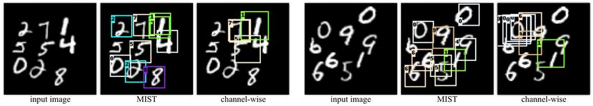
Figure 5: Two qualitative examples for detection and classification on our Multi-MNIST dataset.
unsupervised learning of landmarks. For training details regarding the baselines, see Supplementary
Section B.
Results for “MNIST easy” As shown in Figure 2 (top) all methods successfully re-synthesize the
image, with the exception of Eslami et al. [7]. As this method is sequential, with nine digits the
sequential implementation simply becomes too difficult to optimize through. Note how this method
only learns to describe the scene with a few large regions. We summarize quantitative results in
Table 1.
Results for “MNIST hard” As shown in Figure 2 (bottom), all baseline methods failed to properly
represent the image. Only MIST succeeded at both localizing digits and reconstructing the original
image. Although the grid method accurately reconstructs the image, it has no concept of individual
digits Conversely, as shown in Figure 3, Our method generates accurate bounding boxes for digits
even when these digits overlap, and does so without any location supervision. For quantitative results,
please see Table 1.
Finding the basis of a procedural texture We further demonstrate that our methods can be used
to find the basis function of a procedural texture. For this experiment we synthesize textures with
procedural Gabor noise [21]. Gabor noise is obtained by convolving oriented Gabor wavelets with a
Poisson impulse process. Hence, given exemplars of noise, our framework is tasked to regress the
underlying impulse process and reconstruct the Gabor kernels so that when the two are convolved, we
can reconstruct the original image. Figure 4 illustrates the results of our experiment. The auto-encoder
learned to accurately reconstruct the Gabor kernels, even though in the training images they are
heavily overlapped. These results show that MIST is capable of generating and reconstructing large
numbers of instances per image, which is simply intractable with other approaches.
MIST Grid Ch.-wise [7] [46] MIST Ch.-wise Supervised
MNIST easy .038 .039 .042 .100 .169 IOU 50% 84.6% 25.4% 99.6%
MNIST hard .053 .062 .128 .154 .191 Classif. 95.6% 75.5% 98.7%
Gabor .095 - - - - Both 83.5% 24.8% 98.6%
Table 1: Reconstruction error (root mean square error). Table 2: Instance level detection and clas-
Note that the grid method does not learn any notion of sification performance on the MNIST hard
digits. dataset.
7MIST Supervised
IoU=.00
AP 82.6% 65.6%
APIoU=.50 76.5% 62.8%
APIoU=.60 63.7% 59.8%
APIoU=.70 42.7% 51.9%
APIoU=.80 19.9% 34.6%
APIoU=.90 4.2% 11.0%
Figure 6: Qualitative SVHN results. Table 3: Quantitative SVHN results.
5.2 Multiple instance classification
Multi-MNIST – Figure 5. To test our method in a multiple instance classification setup, we rely on
the MNIST hard dataset. We compare our method to channel-wise, as other baselines are designed
for generative tasks. To evaluate the detection accuracy of the models, we compute the intersection
over union (IoU) between the ground-truth bounding box and the detection results, and assign it
as a match if the IoU score is over 50%. We report the number of correctly classified matches in
Table 2, as well as the proportion of instances that are both correctly detected and correctly classified.
Our method clearly outperforms the channel-wise strategy. Note that, even without localization
supervision, our method correctly localizes digits. Conversely, the channel-wise strategy fails to learn.
This is because multiple instances of the same digits are present in the image. For example, in the
example2 Figure 5 (right), we have two number sizes, zeros, and nines. This prevents any of these
digits from being detected/classified properly by a channel-wise approach.
SVHN – Figure 6 and Table 3. We further apply MIST to the uncropped and unaligned Street View
House Numbers dataset [24]. Compared to previous work that has used cropped and resized SVHN
images (e.g. [1, 11, 17, 24]), this evaluating setting is significantly more challenging, because digits
can appear anywhere in the image. We resize all images to 60 × 240, use only images labeled as
containing 2 digits, and apply MIST at a single scale. Although the dataset provides bounding boxes
for the digits, we ignore these bounding boxes and use only digit labels as supervision. During testing,
we exclude images with small bounding boxes (< 30 pixels in height). We report results in terms
of APIoU=.X , where X is the threshold for determining detection correctness. With IoU = 0, we refer
to a “pure” classification task (i.e. no localization). As shown, supervised results provide better
performance with higher thresholds, but MIST performs even better than the supervised baseline for
moderate thresholds. We attribute this to the fact that, by providing direct supervision on the location,
the training focuses too much on having high localization accuracy.
6 Conclusion
In this paper, we introduce the MIST framework for multi-instance image reconstruction/classification.
Both these tasks are based on localized analysis of the image, yet we train the network without
providing any localization supervision. The network learns how to extract patches on its own, and
these patches are then fed to a task-specific network to realize an end goal. While at first glance the
MIST framework might appear non-differentiable, we show how via lifting they can be effectively
trained in an end-to-end fashion. We demonstrated the effectiveness of MIST by introducing a
variant of the MNIST dataset, and demonstrating compelling performance in both reconstruction and
classification. We also show how the network can be trained to reverse engineer a procedural texture
synthesis process. MISTs are a first step towards the definition of optimizable image-decomposition
networks that could be extended to a number of exciting unsupervised learning tasks. Amongst these,
we intend to explore the applicability of MISTs to unsupervised detection/localization of objects,
facial landmarks, and local feature learning.
Acknowledgements
This work was partially supported by the Natural Sciences and Engineering Research Council
of Canada (NSERC) Discovery Grant “Deep Visual Geometry Machines” (RGPIN-2018-03788,
DGECR-2018-00426), Google, and by systems supplied by Compute Canada.
8References
[1] J. L. Ba, V. Mnih, and K. Kavukcuoglu. Multiple Object Recognition With Visual Attention. In ICLR,
2015.
[2] H. Bay, A. Ess, T. Tuytelaars, and L. Van Gool. SURF: Speeded Up Robust Features. CVIU, 10(3):346–359,
2008.
[3] R. Bridson. Fast Poisson Disk Sampling in Arbitrary Dimensions. In SIGGRAPH sketches, 2007.
[4] Y.-W. Chao, S. Vijayanarasimhan, B. Seybold, D. A. Ross, J. Deng, and R. Sukthankar. Rethinking the
Faster R-CNN Architecture for Temporal Action Localization. In CVPR, 2018.
[5] D. Detone, T. Malisiewicz, and A. Rabinovich. Superpoint: Self-Supervised Interest Point Detection and
Description. CVPR Workshop on Deep Learning for Visual SLAM, 2018.
[6] P. Dollár, C. Wojek, B. Schiele, and P. Perona. Pedestrian Detection: An Evaluation of the State of the Art.
PAMI, 34(4):743–761, 2012.
[7] S. M. A. Eslami, N. Heess, T. Weber, Y. Tassa, D. Szepesvari, K. Kavukcuoglu, and G. E. Hinton. Attend,
Infer, Repeat: Fast Scene Understating with Generative Models. In NeurIPS, 2015.
[8] P. Felzenszwalb, R. Girshick, D. McAllester, and D. Ramanan. Object Detection with Discriminatively
Trained Part Based Models. PAMI, 32(9):1627–1645, 2010.
[9] M. Gao, A. Li, V. I. Morariu, and L. S. Davis. C-WSL: Coung-guided Weakly Supervised Localization. In
ECCV, 2018.
[10] G. Georgakis, S. Karanam, Z. Yu, J. Ernst, and J. Košecká. End-to-end Learning of Keypoint Detector and
Descriptor for Pose Invariant 3D Matching. In CVPR, 2018.
[11] I. Goodfellow, Y. Bularov, J. Ibarz, S. Arnoud, and V. Shet. Multi-digit Number Recognition from Street
View Imagery using Deep Convolutional Neural Networks. In ICLR, 2014.
[12] K. Gregor, I. Danihelka, A. Graves, D. Rezende, and D. Wierstra. DRAW: A Recurrent Neural Network
For Image Generation. In ICML, 2015.
[13] A. Gupta, A. Vedaldi, and A. Zisserman. Inductive Visual Localization: Factorised Training for Superior
Generalization. In BMVC, 2018.
[14] K. He, G. Gkioxari, P. Dollar, and R. Girshick. Mask R-CNN. In ICCV, 2017.
[15] K. He, X. Zhang, R. Ren, and J. Sun. Delving Deep into Rectifiers: Surpassing Human-Level Performance
on Imagenet Classification. In ICCV, 2015.
[16] N. Inoue, R. Furuta, T. Yamasaki, and K. Aizawa. Cross-Domain Weakly-Supervised Object Detection
through Progressive Domain Adaptation. In ECCV, 2018.
[17] M. Jaderberg, K. Simonyan, A. Zisserman, and K. Kavukcuoglu. Spatial Transformer Networks. In
NeurIPS, pages 2017–2025, 2015.
[18] W. Jiang, W. Sun, A. Tagliasacchi, E. Trulls, and K. M. Yi. Linearized multi-sampling for differentiable
image transformation. arXiv Preprint, 2019.
[19] J. Johnson, A. Gupta, and L. Fei-fei. Image Generation from Scene Graphs. In CVPR, 2018.
[20] J. Johnson, A. Karpathy, and L. Fei-fei. Densecap: Fully Convolutional Localization Networks for Dense
Captioning. In CVPR, 2016.
[21] A. Lagae, S. Lefebvre, G. Drettakis, and Ph. Dutré. Procedural noise using sparse gabor convolution. TOG,
2009.
[22] D. Lowe. Distinctive Image Features from Scale-Invariant Keypoints. IJCV, 20(2), 2004.
[23] D. Merget, M. Rock, and G. Rigoll. Robust Facial Landmark Detection via a Fully-Conlolutional Local-
Global Context Network. In CVPR, 2018.
[24] Y. Netzer, T. Wang, A. Coates, A. Bissacco, B. Wu, and A. Y. Ng. Reading digits in natural images with
unsupervised feature learning. Deep Learning and Unsupervised Feature Learning Workshop, NeurIPS,
2011.
[25] A. Newell, K. Yang, and J. Deng. Stacked Hourglass Networks for Human Pose Estimation. In ECCV,
2016.
[26] Y. Ono, E. Trulls, P. Fua, and K. M. Yi. Lf-Net: Learning Local Features from Images. In NeurIPS, 2018.
[27] J. Redmon, S. Divvala, R. Girshick, and A. Farhadi. You Only Look Once: Unified, Real-Time Object
Detection. In CVPR, 2016.
[28] J. Redmon and A. Farhadi. YOLO 9000: Better, Faster, Stronger. In CVPR, 2017.
[29] S. Ren, K. He, R. Girshick, and J. Sun. Faster R-CNN: Towards Real-Time Object Detection with Region
Proposal Networks. In NeurIPS, 2015.
[30] R. R. Selvaraju, M. Cogswell, A. Das, R. Vedantam, D. Parikh, and D. Batra. Grad-CAM: Visual
Explanations from Deep Networks via Gradient-based Localization. In ICCV, 2017.
[31] R. Sewart and M. Andriluka. End-to-End People Detection in Crowded Scenes. In CVPR, 2016.
[32] B. Singh, H. Li, A. Sharma, and L. S. Davis. R-FCN-3000 at 30fps: Decoupling Detection and Classifica-
tion. In CVPR, 2018.
[33] O. Sorkine and M. Alexa. As-rigid-as-possible surface modeling. In SGP, 2007.
[34] M. Sun, Y. Yuan, F. Zhou, and E. Ding. Multi-Attention Multi-Class Constraint for Fine-grained Image
Recognition. In ECCV, 2018.
[35] S. Suwajanakorn, N. Snavely, J. Tompson, and M. Norouzi. Discovery of Latent 3D Keypoints via
End-To-End Geometric Reasoning. In NeurIPS, 2018.
[36] P. Tang, X. Wang, A. Wang, Y. Yan, W. Liu, J. Huang, and A. Yuille. Weakly Supervised Region Proposal
Network and Object Detection. In ECCV, 2018.
9[37] J. Taylor, L. Bordeaux, T. Cashman, B. Corish, C. Keskin, E. Soto, D. Sweeney, J. Valentin, B. Luff,
A. Topalian, E. Wood, S. Khamis, P. Kohli, T. Sharp, S. Izadi, R. Banks, A. Fitzgibbon, and J. Shot-
ton. Efficient and precise interactive hand tracking through joint, continuous optimization of pose and
correspondences. TOG, 2016.
[38] B. Tekin, P. Marquez-neila, M. Salzmann, and P. Fua. Learning to Fuse 2D and 3D Image Cues for
Monocular Body Pose Estimation. In ICCV, 2017.
[39] J. R. R. Uijlings, S. Popov, and V. Ferrari. Revisiting Knowledge Transfer for Training Object Class
Detectors. In CVPR, 2018.
[40] F. Wan, P. Wei, J. Jiao, Z. Han, and Q. Ye. Min-Entropy Latent Model for Weakly Supervised Object
Detection. In CVPR, 2018.
[41] F. Wang, L. Zhao, X. Li, X. Wang, and D. Tao. Geometry-Aware Scene Text Detection with Instance
Transformation Network. In CVPR, 2018.
[42] K. M. Yi, E. Trulls, V. Lepetit, and P. Fua. LIFT: Learned Invariant Feature Transform. In ECCV, 2016.
[43] C. Zach and G. Bournaoud. Descending, Lifting or Smoothing: Secrets of Robust Cost Opimization. In
ECCV, 2018.
[44] S. Zhang, J. Yang, and B. Schiele. Occluded Pedestrian Detection Through Guided Attention in CNNs. In
CVPR, 2018.
[45] X. Zhang, Y. Wei, G. Kang, Y. Wang, and T. Huang. Self-produced Guidance for Weakly-supervised
Object Localization. In ECCV, 2018.
[46] Y. Zhang, Y. Gui, Y. Jin, Y. Luo, Z. He, and H. Lee. Unsupervised Discovery of Object Landmarks as
Structural Representations. In CVPR, 2018.
[47] B. Zhou, A. Khosla, A. Lapedriza, A. Oliva, and A. Torralba. Learning Deep Features for Discriminative
Localization. In CVPR, 2016.
10Appendix
A Comparison to LF-Net
Note that differently from LF-Net [26], we do not perform a softmax along the scale dimension.
The scale-wise softmax in LF-Net is problematic as the computation for a softmax function relies
on the input to the softmax being unbounded. For example, in order for the softmax function to
behave as a max function, due to exponentiation, it is necessary that one of the input value reaches
infinity (i.e. the value that will correspond to the max), or that all other values to reach negative
infinity. However, at the network stage where softmax is applied in [26], the score range from zero to
one, effectively making the softmax behave similarly to averaging. Our formulation does not suffer
from this drawback.
B Implementation details
MIST auto-encoder network. The input layer of the autoencoder is 32 × 32 × C where C is the
number of color channels. We use 5 up/down-sampling levels. Each level is made of 3 standard
non-bottleneck ResNet v1 blocks [15] and each ResNet block uses a number of channels that doubles
after each downsampling step. ResNet blocks uses 3×3 convolutions of stride 1 with ReLU activation.
For downsampling we use 2D max pooling with 2 × 2 stride and kernel. For upsampling we use 2D
transposed convolutions with 2 × 2 stride and kernel. The output layer uses a sigmoid function, and
we use layer normalization before each convolution layer.
MIST classification network. We re-use the same architecture as encoder for first the task and
append a dense layer to map the latent space to the score vector of our 10 digit classes.
Baseline unsupervised reconstruction methods. To implement the Eslami et al. [7] baseline, we
use a publicly available reimplementation.1 We note that Eslami et al. [7] originally applied their
model to a dataset consisting of images of 0, 1, or 2 digits with equal probability. We found that the
model failed to converge unless it was trained with examples where various number of total digits
exist, so for fair comparison, we populate the training set with images consisting of all numbers of
digits between 0 and 9. For the Zhang et al. [46] baseline, we use the authors’ implementation and
hyperparameters.
C Convergence during training
Figure 7: Evolution of the loss during training. (left) The classification loss. (middle) The heatmap
loss. (right) The heatmap evolution over training iterations (from top to bottom) on an SVHN example
image.
As is typical for neural network training, our objective is non-convex and there is no guarantee that
a local minimum found by gradient descent training is a global minimum. Empirically, however,
the optimization process is stable, as shown in Figure 7. Early in training, keypoints are detected
at random locations as the heatmaps are generated by networks with randomly initialized weights.
1
https://github.com/aakhundov/tf-attend-infer-repeat
1However, as training continues, keypoints that, by chance, land on locations nearby the correct object
(e.g. numbers) for certain samples in the random batch, and become reinforced. Thus, ultimately
MIST learns to detect these locations and perform the task of interest. Note that this is unsurprising,
as our formulation is a lifted version of this loss to allow gradient-based training. Figure 7(right)
also shows the evolution of the heatmap starting from a random-like signal (top) and converging to a
highly peaked response (bottom).
D Non-uniform distributions
Figure 8: Examples with uneven distributions of digits.
Although the images we show in Figure 2 involve small displacements from a uniformly spaced grid,
our method does not require the keypoints to be evenly spread. As shown in Figure 8, our method
is able to successfully learn even when the digits are placed unevenly. Note that, as our detector is
fully convolutional and local, it cannot learn the absolute location of keypoints. In fact, we weakened
the randomness of the locations for fairness against [46], which is not designed to deal with severe
displacements.
2You can also read