Improving Inductive Link Prediction Using Hyper-Relational Facts
←
→
Page content transcription
If your browser does not render page correctly, please read the page content below

Improving Inductive Link Prediction Using
                                                              Hyper-Relational Facts

                                             Mehdi Ali1,2? , Max Berrendorf3? , Mikhail Galkin4 , Veronika Thost5 , Tengfei Ma5 ,
                                                                  Volker Tresp3,6 , and Jens Lehmann1,2
                                                           1
                                                              Smart Data Analytics Group, University of Bonn, Germany
                                                                   {mehdi.ali,jens.lehmann}@cs.uni-bonn.de
arXiv:2107.04894v1 [cs.LG] 10 Jul 2021

                                         2
                                             Fraunhofer Institute for Intelligent Analysis and Information Systems (IAIS), Sankt Augustin
                                                                                 and Dresden, Germany
                                                                {mehdi.ali,jens.lehmann}@iais.fraunhofer.de
                                                         3
                                                            Ludwig-Maximilians-Universität München, Munich, Germany
                                                                       {berrendorf,tresp}@dbs.ifi.lmu.de
                                                                               4
                                                                                  Mila, McGill University
                                                                            mikhail.galkin@mila.quebec
                                                                     5
                                                                        IBM Research, MIT-IBM Watson AI Lab
                                                                   vth@zurich.ibm.com, tengfei.ma1@ibm.com
                                                                          6
                                                                              Siemens AG, Munich, Germany
                                                                             volker.tresp@siemens.com

                                                  Abstract. For many years, link prediction on knowledge graphs (KGs) has been
                                                  a purely transductive task, not allowing for reasoning on unseen entities. Re-
                                                  cently, increasing efforts are put into exploring semi- and fully inductive sce-
                                                  narios, enabling inference over unseen and emerging entities. Still, all these
                                                  approaches only consider triple-based KGs, whereas their richer counterparts,
                                                  hyper-relational KGs (e.g., Wikidata), have not yet been properly studied. In
                                                  this work, we classify different inductive settings and study the benefits of
                                                  employing hyper-relational KGs on a wide range of semi- and fully inductive
                                                  link prediction tasks powered by recent advancements in graph neural networks.
                                                  Our experiments on a novel set of benchmarks show that qualifiers over typed
                                                  edges can lead to performance improvements of 6% of absolute gains (for the
                                                  Hits@10 metric) compared to triple-only baselines. Our code is available at
                                                  https://github.com/mali-git/hyper relational ilp.

                                         1     Introduction
                                         Knowledge graphs are notorious for their sparsity and incompleteness [16], so that
                                         predicting missing links has been one of the first applications of machine learning and
                                         embedding-based methods over KGs [22,9]. A flurry [2,20] of such algorithms has
                                         been developed over the years, and most of them share certain commonalities, i.e., they
                                         operate over triple-based KGs in the transductive setup, where all entities are known
                                         at training time. Such approaches can neither operate on unseen entities, which might
                                         emerge after updating the graph, nor on new (sub-)graphs comprised of completely
                                         ?
                                             equal contribution
2 Ali et al.
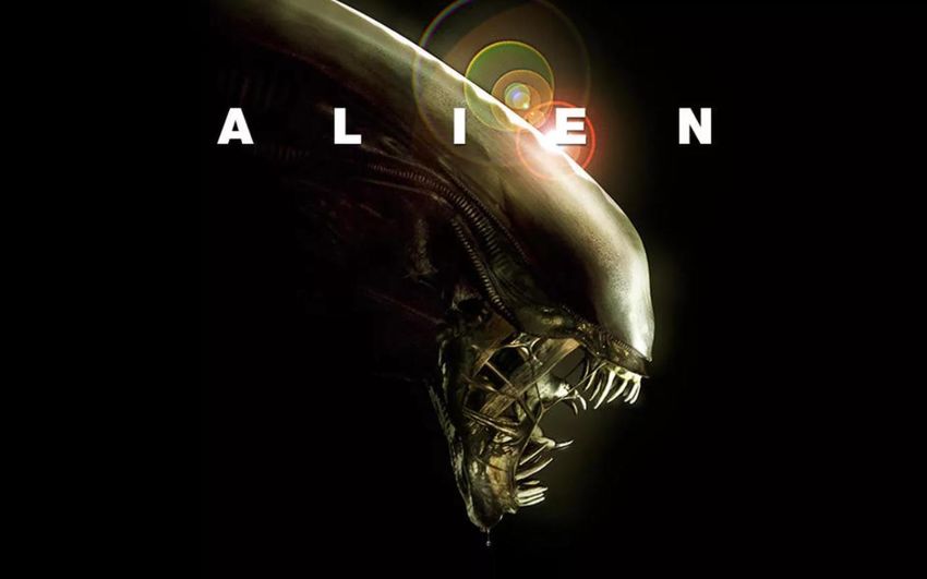
Matt Damon Good Will Hunting Drama
seen Q175535 Q193835 Q130232
graph
cast member genre
P161 P136
unseen
graph Best Actor
Q103916 director
nominated for P57 genre
P1411 P136
Milk
The Martian Q201687
Q18547944 Gus Van Sant
Q76819
nominee (P2453):
Matt Damon(Q175535)
director
P57
director
Alien P57
Q103569
genre
P136 director Ridley Scott Semi-
P57 inductive link
Q56005
Sci-fi genre
Q471839 P136 director Fully-
P57 inductive link
genre Blade Runner
P136 Q184843
Fig. 1. Different types of inductive LP. Semi-inductive: the link between The Martian and Best
Actor from the seen graph. Fully-inductive: the genre link between unseen entities given a new
unseen subgraph at inference time. The qualifier (nominee: Matt Damon) over the original
relation nominated for allows to better predict the semi-inductive link.
new entities. Those scenarios are often unified under the inductive link prediction (LP)
setup. A variety of NLP tasks building upon KGs have inductive nature, for instance,
entity linking or information extraction. Hence, being able to work in inductive settings
becomes crucial for KG representation learning algorithms. For instance (cf. Fig. 1), the
director-genre pattern from the seen graph allows to predict a missing genre link for
The Martian in the unseen subgraph.
Several recent approaches [24,13] tackle an inductive LP task, but they usually
focus on a specific inductive setting. Furthermore, their underlying KG structure is
still based on triples. On the other hand, new, more expressive KGs like Wikidata [26]
exhibit a hyper-relational nature where each triple (a typed edge in a graph) can be
further instantiated with a set of explicit relation-entity pairs, known as qualifiers in the
Wikidata model. Recently, it was shown [17] that employing hyper-relational KGs yields
significant gains in the transductive LP task compared to their triple-only counterparts.
But the effect of such KGs on inductive LP is unclear. Intuitively (Fig. 1), the (nominee:
Matt Damon) qualifier provides a helpful signal to predict Best Actor as an object
of nominated for of The Martian given that Good Will Hunting received such an
award with the same nominee.
In this work, we systematically study hyper-relational KGs in different inductive
settings:
Improving Inductive Link Prediction Using Hyper-Relational Facts         3

– We propose a classification of inductive LP scenarios that describes the settings
  formally and, to the best of our knowledge, integrates all relevant existing works.
  Specifically, we distinguish fully-inductive scenarios, where target links are to be
  predicted in a new subgraph of unseen entities, and semi-inductive ones where unseen
  nodes have to be connected to a known graph.
– We then adapt two existing baseline models for the two inductive LP tasks probing
  them in the hyper-relational settings.
– Our experiments suggest that models supporting hyper-relational facts indeed improve
  link prediction in both inductive settings compared to strong triple-only baselines by
  more than 6% Hits@10.

2      Background
We assume the reader to be familiar with the standard link prediction setting (e.g.
from [22]) and introduce the specifics of the setting with qualifiers.

2.1     Statements: Triples plus Qualifiers
Let G = (E, R, S) be a hyper-relational KG where E is a set of entities, R is a set
of relations, and S a set of statements. Each statement can be formalized as a 4-tuple
(h, r, t, q) of a head and tail entity7 h, t ∈ E, a relation r ∈ R, and a set of qualifiers,
which are relation-entity pairs q ⊆ P(R × E) where P denotes the power set. For
example, Fig. 1 contains a statement (Good Will Hunting, nominated for, Best
Actor, {(nominee, Matt Damon)}) where (nominee, Matt Damon) is a qualifier
pair for the main triple. We define the set of all possible statements as set
                     S(EH , R, ET , EQ ) = EH × R × ET × P(R × EQ )
with a set of relations R, a set of head, tail and qualifier entities EH , ET , EQ ⊆ E. Further,
Strain is the set of training statements and Seval are evaluation statements. We assume
that we have a feature vector xe ∈ Rd associated with each entity e ∈ E. Such feature
vectors can, for instance, be obtained from entity descriptions available in some KGs
or represent topological features such as Laplacian eigenvectors [6] or regular graph
substructures [10]. In this work, we focus on the setting with one fixed set of known
relations. That is, we do not require xr ∈ Rd features for relations and rather learn
relation embeddings during training.

2.2     Expressiveness
Models making use of qualifiers are strictly more expressive than those which do
not: Consider the following example with two statements, s1 = (h, r, t, q1 ) and s2 =
(h, r, t, q2 ), sharing the same triple components, but differing in their qualifiers, such
that s1 |q1 = F alse and s2 |q2 = T rue. For a model fN Q not using qualifiers, i.e., only
using the triple component (h, r, t), we have fN Q (s1 ) = fN Q (s2 ). In contrast, a model
fQ using qualifiers can predict fQ (s1 ) 6= fQ (s2 ), thus being strictly more expressive.
 7
     We use entity and node interchangeably
4        Ali et al.

Named scenario             Sinf           Unseen ↔ Unseen Unseen ↔ Seen Scoring against In our framework
Out-of-sample [1]          k-shot                -               X            Etr              SI
Unseen entities [12]       k-shot                -               X            Etr              SI
Inductive [8]              k-shot                -               X            Etr              SI
Inductive [24]           new graph               X               -            Einf             FI
Transfer [13]            new graph               X               -            Einf             FI
Dynamic [13]         k-shot + new graph          X               X         Etr ∪ Einf        FI / SI
Out-of-graph [4]     k-shot + new graph          X               X         Etr ∪ Einf        FI / SI
Inductive [27]       k-shot + new graph          X               X         Etr ∪ Einf        FI / SI
Table 1. Inductive LP in the literature, a discrepancy in terminology. The approaches differ in
the kind of auxiliary statements Sinf used at inference time: in whether they contain entities seen
during training Etr and whether new entities Einf are connected to seen ones (k-shot scenario), or
(only) amongst each other, in a new graph. Note that the evaluation settings also vary.

3    Inductive Link Prediction
Recent works (cf. Table 1) have pointed out the practical relevance of different inductive
LP scenarios. However, there exists a terminology gap as different authors employ
different names for describing conceptually the same task or, conversely, use the same
inductive LP term for practically different setups. We propose a unified framework that
provides an overview of the area and describes the settings formally.
     Let E• denote the set of entities occurring in the training statements Strain at any
position (head, tail, or qualifier), and E◦ ⊆ E \ E• denote a set of unseen entities. In the
transductive setting, all entities in the evaluation statements are seen during training, i.e.,
Seval ⊆ S(E• , R, E• , E• ). In contrast, in inductive settings, Seval , used in validation and
testing, may contain unseen entities. In order to be able to learn representations for these
entities at inference time, inductive approaches may consider an additional set Sinf of
inference statements about (un)seen entities; of course Sinf ∩ Seval = ∅.
     The fully-inductive setting (FI) is akin to transfer learning where link prediction is
performed over a set of entities not seen before, i.e., Seval ⊆ S(E◦ , R, E◦ , E◦ ). This
is made possible by providing an auxiliary inference graph Sinf ⊆ S(E◦ , R, E◦ , E◦ )
containing statements about the unseen entities in Seval . For instance, in Fig. 1, the
training graph is comprised of entities Matt Damon, Good Will Hunting, Best
Actor, Gus Van Sant, Milk, Drama. The inference graph contains new entities The
Martian, Alien, Ridley Scott, Blade Runner, Sci-fi with one missing link to
be predicted. The fully-inductive setting is considered in [24,13].
     In the semi-inductive setting (SI), new, unseen entities are to be connected to seen
entities, i.e., Seval ⊆ S(E• , R, E◦ , E• ) ∪ S(E◦ , R, E• , E• ). Illustrating with Fig. 1, The
Martian as the only unseen entity connecting to the seen graph, the semi-inductive
statement connects The Martian to the seen Best Actor. Note that there are other
practically relevant examples beyond KGs, such as predicting interaction links between
a new drug and a graph containing existing proteins/drugs [5,18]. We hypothesize that,
in most scenarios, we are not given any additional information about the new entity, and
thus have Sinf = ∅; we will focus on this case in this paper. However, the variation
where Sinf may contain k statements connecting the unseen entity to seen ones has been
considered too [1,8,12] and is known as k-shot learning scenario.
Improving Inductive Link Prediction Using Hyper-Relational Facts 5
A mix of the fully- and semi-inductive settings where evaluation statements may
contain two instead of just one unseen entity is studied in [13,4,27]. That is, unseen
entities might be connected to the seen graph, i.e., Seval may contain seen entities, and,
at the same time, the unseen entities might be connected to each other; i.e, Sinf 6= ∅.
Our framework is general enough to allow Seval to contain new, unseen relations r
having their features xr at hand. Still, to the best of our knowledge, research so far has
focused on the setting where all relations are seen in training; we will do so, too.
We hypothesize that qualifiers, being explicit attributes over typed edges, provide a
strong inductive bias for LP tasks. In this work, for simplicity, we require both qualifier
relations and entities to be seen in the training graph, i.e., EQ ⊆ E• and RQ ⊆ R,
although the framework accommodates a more general case of unseen qualifiers given
their respective features.
4 Approach
Both semi- and fully-inductive tasks assume node features to be given. Recall that
relation embeddings are learned and, often, to reduce the computational complexity,
their dimensionality is smaller than that of node features.
4.1 Encoders
In the semi-inductive setting, an unseen entity arrives without any graph structure point-
ing to existing entities, i.e., Sinf = ∅. This fact renders message passing approaches [19]
less applicable, so we resort to a simple linear layer to project all entity features (includ-
ing those of qualifiers) into the relation space: φ : Rdf → Rdr
In the fully inductive setting, we are given a non-empty inference graph Sinf 6= ∅,
and we probe two encoders: (i) the same linear projection of features as in the semi-
inductive scenario which does not consider the graph structure; (ii) GNNs which can
naturally work in the inductive settings [11]. However, the majority of existing GNN
encoders for multi-relational KGs like CompGCN [25] are limited to only triple KG
representation. To the best of our knowledge, only the recently proposed S TAR E [17]
encoder supports hyper-relational KGs which we take as a basis for our inductive model.
Its aggregation formula is:
X
x0v = f Wλ(r) φr (xu , γ(xr , xq )vu ) (1)
(u,r)∈N (v)
where γ is a function that infuses the vector of aggregated qualifiers xq into the vector of
the main relation xr . The output of the GNN contains updated node and relation features
based on the adjacency matrix A and qualifiers Q:
X0 , R0 = S TAR E(A, X, R, Q)
Finally, in both inductive settings, we linearize an input statement in a sequence using
a padding index where necessary: [x0h , x0r , x0q1r , x0q1e , [PAD], . . .]. Note that statements
can greatly vary in length depending on the amount of qualifier pairs, and padding
mitigates this issue.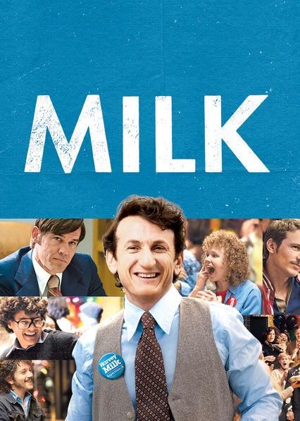
6            Ali et al.

                                   Train                 Validation                  Test                      Inference
Type Name
                              Str (Q%)     Etr Rtr    Svl (Q%) Evl Rvl          Sts (Q%) Ets Rts           Sinf (Q%) Einf Rinf
    SI   WD20K (25)       39,819 ( 30%) 17,014 362 4,252 ( 25%) 3544   194   3,453 ( 22%)   3028   198              -      -   -
    SI   WD20K (33)       25,862 ( 37%) 9251 230 2,423 ( 31%) 1951      88   2,164 ( 28%)   1653    87              -      -   -
    FI   WD20K (66) V1     9,020 ( 85%) 6522 179 910 ( 45%) 1516       111   1,113 ( 50%)   1796   110   6,949 ( 49%)   8313 152
    FI   WD20K (66) V2     4,553 ( 65%) 4269 148 1,480 ( 66%) 2322      79   1,840 ( 65%)   2700    89   8,922 ( 58%)   9895 120
    FI   WD20K (100) V1    7,785 (100%) 5783 92 295 (100%) 643          43     364 (100%)    775    43   2,667 (100%)   4218 75
    FI   WD20K (100) V2    4,146 (100%) 3227 57 538 (100%) 973          43     678 (100%)   1212    42   4,274 (100%)   5573 54
Table 2. Semi-inductive (SI) and fully-inductive (FI) datasets. Sds (Q%) denotes the number of
statements with the qualifiers ratio in train (ds = tr), validation (ds = vl), test (ds = ts), and
inductive inference (ds = inf ) splits. Eds is the number of distinct entities. Rds is the number of
distinct relations. Sinf is a basic graph for vl and ts in the FI scenario.

4.2       Decoder

Given an encoded sequence, we use the same Transformer-based decoder for all settings:

                               f (h, r, t, q) = g(x0h , x0r , x0q1r , x0q1e , . . .)T x0t with
                           g(x01 , . . . , xk ) = Agg(Transformer([x01 , . . . , x0k ]))

    In this work, we evaluated several aggregation strategies and found a simple mean
pooling over all non-padded sequence elements to be preferable. Interaction functions
of the form f (h, r, t, q) = f1 (h, r, q)T f2 (t) are particularly well-suited for fast 1-N
scoring for tail entities, since the first part only needs to be computed only once.
    Here and below, we denote the linear encoder + Transformer decoder model as
QBLP (that is, Qualifier-aware BLP, an extension of BLP [13]), and the S TAR E encoder
+ Transformer decoder, as S TAR E.

4.3       Training

In order to compare results with triple-only approaches, we train the models, as usual, on
the subject and object prediction tasks. We use stochastic local closed world assumption
(sLCWA) and the local closed world assumption (LCWA) commonly used in the KG
embedding literature [2]. Particular details on sLCWA and LCWA are presented in
Appendix A. Importantly, in the semi-inductive setting, the models score against all
entities in the training graph Etr in both training and inference stages. In the fully-
inductive scenario, as we are predicting links over an unseen graph, the models score
against all entities in Etr during training and against unseen entities in the inference
graph Einf during inference.

5        Datasets

We take the original transductive splits of the WD50K [17] family of hyper-relational
datasets as a leakage-free basis for sampling our semi- and fully-inductive datasets which
we denote by WD20K.
Improving Inductive Link Prediction Using Hyper-Relational Facts         7

5.1   Fully-Inductive Setting

We start with extracting statement entities E 0 , and sample n entities and their k-hop
neighbourhood to form the statements (h, r, t, q) of the transductive train graph Strain .
From the remaining E 0 \ Etrain and S \ Strain sets we sample m entities with their
l-hop neighbourhood to form the statements Sind of the inductive graph. The entities
of Sind are disjoint with those of the transductive train graph. Further, we filter out all
statements in Sind whose relations (main or qualifier) were not seen in Strain . Then,
we randomly split Sind with the ratio about 55%/20%/25% into inductive inference,
validation, and test statements, respectively. The evaluated models are trained on the
transductive train graph Strain . During inference, the models receive an unseen inductive
inference graph from which they have to predict validation and test statements. Varying
k and l, we sample two different splits: V1 has a larger training graph with more seen
entities whereas V2 has a bigger inductive inference graph.

5.2   Semi-Inductive Setting

Starting from all statements, we extract all entities occurring as head or tail entity
in any statement, denoted by E 0 and named statement entities. Next, we split the set
of statement entities into a train, validation and test set: Etrain , Evalidation , Etest . We
then proceed to extract statements (h, r, t, q) ∈ S with one entity (h/t) in Etrain and
the other entity in the corresponding statement entity split. We furthermore filter the
qualifiers to contain only pairs where the entity is in a set of allowed entities, formed by
Asplit = Etrain ∪ Esplit , with split being train/validation/test. Finally, since we do not
assume relations to have any features, we do not allow unseen relations. We thus filter
out relations which do not occur in the training statements.

5.3   Overview

To measure the effect of hyper-relational facts on both inductive LP tasks, we sample
several datasets varying the ratio of statements with and without qualifiers. In order to
obtain the initial node features we mine their English surface forms and descriptions
available in Wikidata as rdfs:label and schema:description values. The surface
forms and descriptions are concatenated into one string and passed through the Sentence
BERT [23] encoder based on RoBERTa [21] to get 1024-dimensional vectors. The
overall datasets statistics is presented in Table 2.

6     Experiments

We design our experiments to investigate whether the incorporation of qualifiers im-
proves inductive link prediction. In particular, we investigate the fully-inductive setting
(Section 6.2) and the semi-inductive setting (Section 6.3). We analyze the impact of the
qualifier ratio (i.e., the number of statements with qualifiers) and the dataset’s size on a
model’s performance.
8         Ali et al.

                             WD20K (100) V1                         WD20K (100) V2
Model      #QP
                 AMR(%) MRR(%) H@1(%) H@5(%) H@10(%) AMR(%) MRR(%) H@1(%) H@5(%) H@10(%)
BLP     0         22.78    5.73   1.92   8.22    12.33   36.71   3.99    1.47   4.87   9.22
CompGCN 0         37.02   10.42   5.75   15.07   18.36   74.00   2.55    0.74   3.39   5.31
QBLP    0         28.91   5.52    1.51   8.08    12.60   35.38   4.94    2.58   5.46   9.66
StarE       2     41.89    9.68   3.73   16.57   20.99   40.60   2.43    0.45   3.86   6.17
StarE       4     35.33   10.41   4.82   15.84   21.76   37.16   5.12    1.41   7.93   12.89
StarE       6     34.86   11.27   6.18   15.93   21.29   47.35   4.99    1.92   6.71   11.06
QBLP        2     18.91   10.45   3.73   16.02   22.65   28.03   6.69    3.49   8.47   12.04
QBLP        4     20.19   10.70   3.99   16.12   24.52   31.30   5.87    2.37   7.85   13.93
QBLP        6     23.65   7.87    2.75   10.44   17.86   34.35   6.53    2.95   9.29   13.13
Table 3. Results on FI WD20K (100) V1 & V2. #QP denotes the number of qualifier pairs used in
each statement (including padded pairs). Best results in bold, second best underlined.

                              WD20K (66) V1                         WD20K (66) V2
Model      #QP
                 AMR(%) MRR(%) H@1(%) H@5(%) H@10(%) AMR(%) MRR(%) H@1(%) H@5(%) H@10(%)
BLP     0         34.96   2.10    0.45    2.29   4.44    45.29   1.56    0.27   1.88   3.35
CompGCN 0         35.99   5.80    2.38    8.93   12.79   47.24   2.56    1.17   3.07   4.46
QBLP    0         35.30   3.69    1.30    4.85   7.14    42.48   0.94    0.08   0.79   1.82
StarE       2     37.72   6.84    3.24    9.71   13.44   52.78   2.62    0.74   3.55   5.78
StarE       4     38.91   6.40    2.83    8.94   13.39   51.93   5.06    2.09   7.34   9.82
StarE       6     38.20   6.87    3.46    8.98   13.57   47.01   4.42    2.04   5.73   8.97
QBLP        2     30.37   3.70    1.26    4.90   8.14    53.67   1.39    0.41   1.66   2.59
QBLP        4     30.84   3.20    0.90    4.00   7.14    37.10   2.08    0.38   2.20   4.92
QBLP        6     26.34   4.34    1.66    5.53   9.25    39.12   1.95    0.41   2.15   4.10
Table 4. Results on the FI WD20K (66) V1 & V2. #QP denotes the number of qualifier pairs used
in each statement (including padded pairs). Best results in bold, second best underlined.

6.1     Experimental Setup

We implemented all approaches in Python building upon the open-source library pykeen [3]
and make the code publicly available.8 For each setting (i.e., dataset + number of qualifier
pairs per triple), we performed a hyperparameter search using early stopping on the
validation set and evaluated the final model on the test set. We used AMR, MRR, and
Hits@k as evaluation metrics, where the Adjusted Mean Rank (AMR) [7] is a recently
proposed metric which sets the mean rank into relation with the expected mean rank of a
random scoring model. Its value ranges from 0%-200%, and a lower value corresponds
to better model performance. Each model was trained at most 1000 epochs in the fully
inductive setting, at most 600 epochs in the semi-inductive setting, and evaluated based
on the early-stopping criterion with a frequency of 1, a patience of 200 epochs (in the
semi-inductive setting, we performed all HPOs with a patience of 100 and 200 epochs),
and a minimal improvement δ > 0.3% optimizing the hits@10 metric. For both induc-
tive settings, we evaluated the effect of incorporating 0, 2, 4, and 6 qualifier pairs per
triple.

 8
     https://github.com/mali-git/hyper relational ilp
Improving Inductive Link Prediction Using Hyper-Relational Facts          9

6.2   Fully-Inductive Setting

In the full inductive setting, we analyzed the effect of qualifiers for four different datasets
(i.e., WD20K (100) V1 & V2 and WD20K (66) V1 & V2, which have different ratios of
qualifying statements and are of different sizes (see Section 5). As triple-only baselines,
we evaluated CompGCN [25] and BLP [13]. To evaluate the effect of qualifiers on the
fully-inductive LP task, we evaluated StarE [17] and QBLP. It should be noted that StarE
without the use of qualifiers is equivalent to CompGCN.
     General Overview. Tables 3-4 show the results obtained for the four datasets. The
main findings are that (i) for all datasets, the use of qualifiers leads to increased perfor-
mance, and (ii) the ratio of statements with qualifiers and the size of the dataset has a
major impact on the performance. CompGCN and StarE apply message-passing to obtain
enriched entity representations while BLP and QBLP only apply a linear transformation.
Consequently, CompGCN and StarE require Sinf to contain useful information in order
to obtain the entity representations while BLP and QBLP are independent of Sinf . In the
following, we discuss the results for each dataset in detail.
     Results on WD20K (100) FI V1 & V2. It can be observed that the performance gap
between BLP/QBLP (0) and QBLP (2,4,6) is considerably larger than the gap between
CompGCN and StarE. This might be explained by the fact that QBLP does not take into
account the graph structure provided by Sinf , therefore is heavily dependent on additional
information, i.e. the qualifiers compensate for the missing graph information. The overall
performance decrease observable between V1 and V2 could be explained by the datasets’
composition (Table 2), in particular, in the composition of the training and inference
graphs: Sinf of V2 comprises more entities than V1, so that each test triple is ranked
against more entities, i.e., the ranking becomes more difficult. At the same time, the
training graph of V1 is larger than that of V2, i.e., during training more entities (along
their textual features) are seen which may improve generalization.
     Results on WD20K (66) FI V1 & V2. Comparing StarE (2,4) to CompGCN (0),
there is only a small improvement on this dataset. Also, the improvement of QBLP
(2,4,6) compared to BLP and QBLP (0) is smaller than on the previous datasets. This can
be connected to the decreased ratio of statements with qualifiers. Besides, the training
graph also has fewer qualifier pairs, Sinf which is used by CompGCN and StarE for
message passing consists of only 49% of statements with at least one qualifier pair, and
only 50% of test statements have at least one qualifier pair which has an influence on
all models. This observation supports why StarE outperforms QBLP as the amount of
provided qualifier statements cannot compensate for the graph structure in Sinf .

6.3   Semi-inductive Setting

In the semi-inductive setting, we evaluated BLP as a triple-only baseline and QBLP
as a statement baseline (i.e., involving qualifiers) on the WD20K SI datasets. We did
not evaluate CompGCN and StarE since message-passing-based approaches are not
directly applicable in the absence of Sinf . The results highlight that aggregating qualifier
information improves the prediction of semi-inductive links despite the fact that the ratio
of statements with qualifiers is not very large (37% for SI WD20K (33), and 30% for
SI WD20K (25)). In the case of SI WD20K (33), the baselines are outperformed even
10       Ali et al.

                          WD20K (33) SI                                                 WD20K (25) SI
Model #QP
            AMR(%) MRR(%) H@1(%) H@5(%) H@10(%) AMR(%) MRR(%) H@1(%) H@5(%) H@10(%)
BLP     0    4.76     13.95        7.37       17.28       24.65         6.01      12.45     5.98   17.29   23.43
QBLP    0    7.04     28.35       14.44       28.58       36.32         6.75      17.02     8.82   22.10   29.50
QBLP    2    11.51    35.95       20.70       34.98       41.82         5.99      20.36    11.77   24.86   32.26
QBLP    4    11.38    34.35       19.41       33.90       40.20         12.18     21.05    12.32   24.07   30.09
QBLP    6     4.98    25.94       15.20       30.06       38.70         5.73      19.50    11.14   24.73   31.60
Table 5. Results on the WD20K SI datasets. #QP denotes the number of qualifier pairs used in
each statement (including padded pairs).Best results in bold, second best underlined.

by a large margin. Overall, the results might indicate that in semi-inductive settings,
performance improvements can already be obtained with a decent amount of statements
with qualifiers.

                                10000
                                8000
                                6000
                         rank

                                4000
                                2000
                                   0
                                          0            1         2           3      4
                                                      number of qualifier pairs

Fig. 2. Distribution of individual ranks for head/tail prediction with StarE on WD20K (66) V2.
The statements are grouped by the number of qualifier pairs.

6.4    Qualitative Analysis
We obtain deeper insights on the impact of qualifiers by analyzing the StarE model on
the fully-inductive WD20K (66) V2 dataset. In particular, we study individual ranks
for head/tail prediction of statements with and without qualifiers (cf. Fig. 2) varying
the model from zero to four pairs. First, we group the test statements by the number of
available qualifier pairs. We observe generally smaller ranks which, in turn, correspond
to better predictions when more qualifier pairs are available. In particular, just one
qualifier pair is enough to significantly reduce the individual ranks. Note that we have
less statements with many qualifiers, cf. Appendix D.
    We then study how particular qualifiers affect ranking and predictions. For that, we
measure ranks of predictions for distinct statements in the test set with and without
masking the qualifier relation from the inference graph Sinf . We then compute ∆MR
and group them by used qualifier relations (Fig. 3). Interestingly, certain qualifiers, e.g.,
convicted of or including, deteriorate the performance which we attribute to the
Improving Inductive Link Prediction Using Hyper-Relational Facts 11
×103
4 convicted of
2
including
MR
0
2 statement disputed by
replaces
Qualifying relation
Fig. 3. Rank deviation when masking qualifier pairs containing a certain relation. Transparency is
proportional to the occurrence frequency, bar height/color indicates difference in MR for evaluation
statements using this qualifying relation if the pair is masked. More negative deltas correspond to
better predictions.
usage of rare, qualifier-only entities. Conversely, having qualifiers like replaces reduces
the rank by about 4000 which greatly improves prediction accuracy. We hypothesize it
is an effect of qualifier entities: helpful qualifiers employ well-connected nodes in the
graph which benefit from message passing.
WD20K (100) V1 FI
Wikidata ID relation name ∆MR
P2868 subject has role 0.12
P463 member of -0.04
P1552 has quality -0.34
P2241 reason for deprecation -26.44
P47 shares border with -28.91
P750 distributed by -29.12
WD20K (66) V2 FI
P805 statement is subject of 13.11
P1012 including 5.95
P812 academic major 5.07
P17 country -19.96
P1310 statement disputed by -20.92
P1686 for work -56.87
Table 6. Top 3 worst and best qualifier relations affecting the overall mean rank (the last column).
Negative ∆MR with larger absolute value correspond to better predictions.
Finally, we study the average impact of qualifiers on the whole graph, i.e., we take
the whole inference graph and mask out all qualifier pairs containing one relation and
compare the overall evaluation result on the test set (in contrast to Fig. 3, we count ranks12 Ali et al.
of all test statements, not only those which have that particular qualifier) against the non-
masked version of the same graph. We then sort relations by ∆MR and find top 3 most
confusing and most helpful relations across two datasets (cf. Table 6). On the smaller
WD20K (100) V1 where all statements have at least one qualifier pair, most relations
tend to improve MR. For instance, qualifiers with the distributed by relations reduce
MR by about 29 points. On the larger WD20K (66) V2 some qualifier relations, e.g.,
statement is subject of, tend to introduce more noise and worsen MR which we
attribute to the increased sparsity of the graph given an already rare qualifier entity. That
is, such rare entities might not benefit enough from message passing.
7 Related Work
We focus on semi- and fully inductive link prediction approaches and disregard classical
approaches that are fully transductive, which have been extensively studied in the
literature [2,20].
In the domain of triple-only KGs, both settings have recently received a certain
traction. One of the main challenges for realistic KG embedding is the impossibility of
learning representations of unseen entities since they are not present in the train set.
In the semi-inductive setting, several methods alleviating the issue were proposed.
When a new node arrives with a certain set of edges to known nodes, [1] enhanced the
training procedure such that an embedding of an unseen node is a linear aggregation of
neighbouring nodes. If there is no connection to the seen nodes, [27] propose to densify
the graph with additional edges obtained from pairwise similarities of node features.
Another approach applies a special meta-learning framework [4] when during training
a meta-model has to learn representations decoupled from concrete training entities
but transferable to unseen entities. Finally, reinforcement learning methods [8] were
employed to learn relation paths between seen and unseen entities.
In the fully inductive setup, the evaluation graph is a separate subgraph disjoint with
the training one, which makes trained entity embeddings even less useful. In such cases,
the majority of existing methods [28,12,13,29] resort to pre-trained language models
(LMs) (e.g., BERT [15]) as universal featurizers. That is, textual entity descriptions
(often available in KGs at least in English) are passed through an LM to obtain initial
semantic node features. Nevertheless, mining and employing structural graph features,
e.g., shortest paths within sampled subgraphs, has been shown [24] to be beneficial as
well. This work is independent from the origin of node features and is able to leverage
both, although the new datasets employ Sentence BERT [23] for featurizing.
All the described approaches operate on triple-based KGs whereas our work studies
inductive LP problems on enriched, hyper-relational KGs where we show that incorpo-
rating such hyper-relational information indeed leads to better performance.
8 Conclusion
In this work, we presented a study of the inductive link prediction problem over hyper-
relational KGs. In particular, we proposed a theoretical framework to categorize various
LP tasks to alleviate an existing terminology discrepancy pivoting on two settings,Improving Inductive Link Prediction Using Hyper-Relational Facts 13
namely, semi- and fully-inductive LP. Then, we designed WD20K, a collection of
hyper-relational benchmarks based on Wikidata for inductive LP with a diverse set of pa-
rameters and complexity. Probing statement-aware models against triple-only baselines,
we demonstrated that hyper-relational facts indeed improve LP performance in both
inductive settings by a considerable margin. Moreover, our qualitative analysis showed
that the achieved gains are consistent across different setups and still interpretable.
Our findings open up interesting prospects for employing inductive LP and hyper-
relational KGs along several axes, e.g., large-scale KGs of billions statements, new
application domains including life sciences, drug discovery, and KG-based NLP applica-
tions like question answering or entity linking.
In the future, we plan to extend inductive LP to consider unseen relations and
qualifiers; tackle the problem of suggesting best qualifiers for a statement; and provide
more solid theoretical foundations of representation learning over hyper-relational KGs.
Acknowledgements
This work was funded by the German Federal Ministry of Education and Research
(BMBF) under Grant No. 01IS18036A and Grant No. 01IS18050D (project “MLWin”).
The authors of this work take full responsibilities for its content.
References
1. Albooyeh, M., Goel, R., Kazemi, S.M.: Out-of-sample representation learning for knowledge
graphs. In: Cohn, T., He, Y., Liu, Y. (eds.) Proceedings of the 2020 Conference on Empirical
Methods in Natural Language Processing: Findings, EMNLP 2020, Online Event, 16-20
November 2020. pp. 2657–2666. Association for Computational Linguistics (2020)
2. Ali, M., Berrendorf, M., Hoyt, C.T., Vermue, L., Galkin, M., Sharifzadeh, S., Fischer, A.,
Tresp, V., Lehmann, J.: Bringing light into the dark: A large-scale evaluation of knowledge
graph embedding models under a unified framework. CoRR abs/2006.13365 (2020)
3. Ali*, M., Berrendorf*, M., Hoyt*, C.T., Vermue*, L., Sharifzadeh, S., Tresp, V., Lehmann,
J.: Pykeen 1.0: A python library for training and evaluating knowledge graph embeddings.
Journal of Machine Learning Research 22(82), 1–6 (2021), http://jmlr.org/papers/v22/
20-825.html, * equal contribution
4. Baek, J., Lee, D.B., Hwang, S.J.: Learning to extrapolate knowledge: Transductive few-shot
out-of-graph link prediction. In: Larochelle, H., Ranzato, M., Hadsell, R., Balcan, M., Lin, H.
(eds.) Advances in Neural Information Processing Systems 33: Annual Conference on Neural
Information Processing Systems 2020, NeurIPS 2020, December 6-12, 2020, virtual (2020)
5. Bagherian, M., Sabeti, E., Wang, K., Sartor, M.A., Nikolovska-Coleska, Z., Najarian, K.: Ma-
chine learning approaches and databases for prediction of drug–target interaction: a survey pa-
per. Briefings in Bioinformatics 22(1), 247–269 (01 2020). https://doi.org/10.1093/bib/bbz157,
https://doi.org/10.1093/bib/bbz157
6. Belkin, M., Niyogi, P.: Laplacian eigenmaps and spectral techniques for embedding and clus-
tering. In: Dietterich, T.G., Becker, S., Ghahramani, Z. (eds.) Advances in Neural Information
Processing Systems 14 [Neural Information Processing Systems: Natural and Synthetic, NIPS
2001, December 3-8, 2001, Vancouver, British Columbia, Canada]. pp. 585–591. MIT Press
(2001)14 Ali et al.
7. Berrendorf, M., Faerman, E., Vermue, L., Tresp, V.: Interpretable and fair comparison of link
prediction or entity alignment methods with adjusted mean rank. In: 2020 IEEE/WIC/ACM
International Joint Conference on Web Intelligence and Intelligent Agent Technology (WI-
IAT’20). IEEE (2020)
8. Bhowmik, R., de Melo, G.: Explainable link prediction for emerging entities in knowledge
graphs. In: Pan, J.Z., Tamma, V.A.M., d’Amato, C., Janowicz, K., Fu, B., Polleres, A.,
Seneviratne, O., Kagal, L. (eds.) The Semantic Web - ISWC 2020 - 19th International
Semantic Web Conference. Lecture Notes in Computer Science, vol. 12506, pp. 39–55.
Springer (2020)
9. Bordes, A., Usunier, N., Garcı́a-Durán, A., Weston, J., Yakhnenko, O.: Translating embeddings
for modeling multi-relational data. In: Burges, C.J.C., Bottou, L., Ghahramani, Z., Weinberger,
K.Q. (eds.) Advances in Neural Information Processing Systems 26: 27th Annual Conference
on Neural Information Processing Systems 2013. Proceedings of a meeting held December
5-8, 2013, Lake Tahoe, Nevada, United States. pp. 2787–2795 (2013)
10. Bouritsas, G., Frasca, F., Zafeiriou, S., Bronstein, M.M.: Improving graph neural network
expressivity via subgraph isomorphism counting. CoRR abs/2006.09252 (2020)
11. Chami, I., Abu-El-Haija, S., Perozzi, B., Ré, C., Murphy, K.: Machine learning on graphs: A
model and comprehensive taxonomy. CoRR abs/2005.03675 (2020)
12. Clouatre, L., Trempe, P., Zouaq, A., Chandar, S.: Mlmlm: Link prediction with mean likeli-
hood masked language model (2020)
13. Daza, D., Cochez, M., Groth, P.: Inductive entity representations from text via link prediction
(2020)
14. Dettmers, T., Minervini, P., Stenetorp, P., Riedel, S.: Convolutional 2d knowledge graph
embeddings. In: AAAI. pp. 1811–1818. AAAI Press (2018)
15. Devlin, J., Chang, M., Lee, K., Toutanova, K.: BERT: pre-training of deep bidirectional trans-
formers for language understanding. In: Burstein, J., Doran, C., Solorio, T. (eds.) Proceedings
of the 2019 Conference of the North American Chapter of the Association for Computa-
tional Linguistics: Human Language Technologies, NAACL-HLT 2019, Minneapolis, MN,
USA, June 2-7, 2019, Volume 1 (Long and Short Papers). pp. 4171–4186. Association for
Computational Linguistics (2019)
16. Dong, X., Gabrilovich, E., Heitz, G., Horn, W., Lao, N., Murphy, K., Strohmann, T., Sun,
S., Zhang, W.: Knowledge vault: a web-scale approach to probabilistic knowledge fusion.
In: Macskassy, S.A., Perlich, C., Leskovec, J., Wang, W., Ghani, R. (eds.) The 20th ACM
SIGKDD International Conference on Knowledge Discovery and Data Mining, KDD ’14,
New York, NY, USA - August 24 - 27, 2014. pp. 601–610. ACM (2014)
17. Galkin, M., Trivedi, P., Maheshwari, G., Usbeck, R., Lehmann, J.: Message passing for hyper-
relational knowledge graphs. In: Webber, B., Cohn, T., He, Y., Liu, Y. (eds.) Proceedings of
the 2020 Conference on Empirical Methods in Natural Language Processing, EMNLP 2020,
Online, November 16-20, 2020. pp. 7346–7359. Association for Computational Linguistics
(2020)
18. Gaudelet, T., Day, B., Jamasb, A.R., Soman, J., Regep, C., Liu, G., Hayter, J.B.R., Vickers, R.,
Roberts, C., Tang, J., Roblin, D., Blundell, T.L., Bronstein, M.M., Taylor-King, J.P.: Utilising
graph machine learning within drug discovery and development. CoRR abs/2012.05716
(2020)
19. Gilmer, J., Schoenholz, S.S., Riley, P.F., Vinyals, O., Dahl, G.E.: Neural message passing for
quantum chemistry. In: Precup, D., Teh, Y.W. (eds.) Proceedings of the 34th International
Conference on Machine Learning, ICML 2017, Sydney, NSW, Australia, 6-11 August 2017.
Proceedings of Machine Learning Research, vol. 70, pp. 1263–1272. PMLR (2017)
20. Ji, S., Pan, S., Cambria, E., Marttinen, P., Yu, P.S.: A survey on knowledge graphs: Represen-
tation, acquisition and applications. CoRR abs/2002.00388 (2020)Improving Inductive Link Prediction Using Hyper-Relational Facts 15
21. Liu, Y., Ott, M., Goyal, N., Du, J., Joshi, M., Chen, D., Levy, O., Lewis, M., Zettle-
moyer, L., Stoyanov, V.: Roberta: A robustly optimized BERT pretraining approach. CoRR
abs/1907.11692 (2019), http://arxiv.org/abs/1907.11692
22. Nickel, M., Tresp, V., Kriegel, H.: A three-way model for collective learning on multi-
relational data. In: Getoor, L., Scheffer, T. (eds.) Proceedings of the 28th International
Conference on Machine Learning, ICML 2011, Bellevue, Washington, USA, June 28 - July 2,
2011. pp. 809–816. Omnipress (2011)
23. Reimers, N., Gurevych, I.: Sentence-bert: Sentence embeddings using siamese bert-networks.
In: Proceedings of the 2019 Conference on Empirical Methods in Natural Language Process-
ing. Association for Computational Linguistics (11 2019), https://arxiv.org/abs/1908.
10084
24. Teru, K., Denis, E., Hamilton, W.: Inductive relation prediction by subgraph reasoning. In:
Proceedings of the 37th International Conference on Machine Learning, ICML 2020, 13-18
July 2020, Virtual Event. Proceedings of Machine Learning Research, vol. 119, pp. 9448–9457.
PMLR (2020)
25. Vashishth, S., Sanyal, S., Nitin, V., Talukdar, P.P.: Composition-based multi-relational
graph convolutional networks. In: 8th International Conference on Learning Representa-
tions, ICLR 2020, Addis Ababa, Ethiopia, April 26-30, 2020. OpenReview.net (2020),
https://openreview.net/forum?id=BylA C4tPr
26. Vrandecic, D., Krötzsch, M.: Wikidata: a free collaborative knowledgebase. Commun. ACM
57(10), 78–85 (2014)
27. Wang, B., Wang, G., Huang, J., You, J., Leskovec, J., Kuo, C.J.: Inductive learning on
commonsense knowledge graph completion. CoRR abs/2009.09263 (2020)
28. Yao, L., Mao, C., Luo, Y.: Kg-bert: Bert for knowledge graph completion (2019)
29. Zhang, Z., Liu, X., Zhang, Y., Su, Q., Sun, X., He, B.: Pretrain-kge: Learning knowledge
representation from pretrained language models. In: Cohn, T., He, Y., Liu, Y. (eds.) Pro-
ceedings of the 2020 Conference on Empirical Methods in Natural Language Processing:
Findings, EMNLP 2020, Online Event, 16-20 November 2020. pp. 259–266. Association for
Computational Linguistics (2020)16 Ali et al.
A Training
In the sLCWA, negative training examples are created for each true fact (h, r, t) ∈ KG
by corrupting the head or tail entity resulting in the triples (h0 , r, t)/(h, r, t0 ). In the
LCWA, for each triple (h, r, t) ∈ KG all triples (h, r, t0 ) ∈ / KG are considered as
non-existing, i.e., as negative examples.
Under the sLCWA, we trained the models using the margin ranking loss [9]:
− −
L(f (t+ +
i ), f (ti )) = max(0, λ + f (ti ) − f (ti )) , (2)
−
where f (t+
i ) denotes the model’s score for a positive training example and f (ti ) for
a negative one.
For training under the LCWA, we used the binary cross entropy loss [14]:
L(f (ti ), li ) = − (li · log(σ(f (ti )))
(3)
+ (1 − li ) · log(1 − σ(f (ti )))),
where li corresponds to the label of the triple ti .
B Hyperparameter Ranges
The following tables summarizes the hyper-parameter ranges explored during hyper-
parameter optimization. The best hyper-parameters for each of our 46 ablation studies
will be available online upon publishing.
C Infrastructure and Parameters
We train each model on machines running Ubuntu 18.04 equipped with a GeForce RTX
2080 Ti with 12GB RAM. In total, we performed 46 individual hyperparameter opti-
mizations (one for each dataset / model / number-of-qualifier combination). Depending
on the exact configuration, the individual models have between 500k and 5M parameters
and take up to 2 hours for training.
D Qualifier Ratio
Figure 4 shows the ratio of statements with a given number of available qualifier pairs
for all datasets and splits. We generally observe that there are only few statements with a
large number of qualifier pairs, while most of them have zero to two qualifier pairs.Improving Inductive Link Prediction Using Hyper-Relational Facts 17
Hyper-Parameter Value
GCN layers {2,3}
Embedding dim. {32, 64, ... , 256 }
Transformer hid. dim. {512, 576, ... , 1024 }
Num. attention heads {2, 4}
Num. transformer heads {2, 4}
Num. transformer layers {2, 3, 4}
Qualifier aggr. {sum, attention}
Qualifier weight 0.8
Dropout {0.1, 0.2, ... , 0.5 }
Attention slope {0.1, 0.2, 0.3, 0.4 }
Training approaches {sLCWA, LCWA}
Loss fcts. {MRL, BCEL}
Learning rate (log scale) [0.0001, 1.0)
Label smoothing {0.1, 0.15}
Batch size {128, 192, ... , 1024}
Max Epochs FI setting 1000
Max Epochs SI setting 600
Table 7. Hyperparameter ranges explored during hyper-parameter optimization. FI denotes the
fully-inductive setting and SI the semi-inductive setting. For the sLCWA training approach, we
trained the models with the margin ranking loss (MRL), and with the LCWA we used the BCEL
(Binary Cross Entropy loss
.
name = wd50_100 | split = inductive - v1 name = wd50_100 | split = inductive - v2 name = wd50_100 | split = semi-inductive name = wd50_100 | split = transductive
0.7
0.8 0.7 0.6
0.6
0.6
0.5
0.6 0.5
0.5
0.4
0.4
frequency
0.4
0.4 0.3
0.3 0.3
0.2 0.2
0.2
0.2
0.1 0.1 0.1
0.0 0.0 0.0 0.0
part
name = wd50_66 | split = inductive - v1 name = wd50_66 | split = inductive - v2 name = wd50_66 | split = semi-inductive name = wd50_66 | split = transductive test
0.8 train
0.5 validation
0.5 0.7 0.4
0.4
0.6
0.4
0.5 0.3
0.3
frequency
0.3
0.4
0.2
0.2 0.3
0.2
0.2
0.1 0.1
0.1
0.1
0.0 0.0 0.0 0.0
0 1 2 3 4 5 6 0 1 2 3 4 5 6 0 1 2 3 4 5 6 0 1 2 3 4 5 6
num_qualifier_pairs num_qualifier_pairs num_qualifier_pairs num_qualifier_pairs
Fig. 4. Percentage of statements with the given number of available qualifier pairs for all datasets
and splits.You can also read