Cold-Air Outbreaks in the Marine Boundary Layer Experiment (COMBLE) Field Campaign Report
←
→
Page content transcription
If your browser does not render page correctly, please read the page content below
DOE/SC-ARM-21-001

Cold-Air Outbreaks in the Marine Boundary Layer
Experiment (COMBLE) Field Campaign Report

B Geerts G McFarquhar
L Xue M Jensen
P Kollias M Ovchinnikov
M Shupe P DeMott
Y Wang M Tjernström
P Field S Abel
T Spengler R Neggers
S Crewell M Wendisch
C Lüpkes

January 2021
DISCLAIMER

This report was prepared as an account of work sponsored by the U.S.
Government. Neither the United States nor any agency thereof, nor any of
their employees, makes any warranty, express or implied, or assumes any
legal liability or responsibility for the accuracy, completeness, or
usefulness of any information, apparatus, product, or process disclosed, or
represents that its use would not infringe privately owned rights. Reference
herein to any specific commercial product, process, or service by trade
name, trademark, manufacturer, or otherwise, does not necessarily
constitute or imply its endorsement, recommendation, or favoring by the
U.S. Government or any agency thereof. The views and opinions of
authors expressed herein do not necessarily state or reflect those of the
U.S. Government or any agency thereof.
DOE/SC-ARM-21-001

Cold-Air Outbreaks in the Marine Boundary
Layer Experiment (COMBLE) Field
Campaign Report

B Geerts, University of Wyoming
Principal Investigator

G McFarquhar, University of Oklahoma (UO)
L Xue, National Center for Atmospheric Research
M Jensen, Brookhaven National Laboratory (BNL)
P Kollias, Stony Brook University and BNL
M Ovchinnikov, Pacific Northwest National Laboratory
M Shupe, UO and National Oceanic and Atmospheric Administration
P DeMott, Colorado State University
Y Wang, State University of New York, Oswego
M Tjernström, Stockholm University
P Field, United Kingdom Meteorological Office (UK Met Office)
S Abel, UK Met Office
T Spengler, University of Bergen
R Neggers, University of Cologne (UC)
S Crewell, UC
M Wendisch, University of Leipzig
C Lüpkes, Alfred Wegener Institute
Co-Investigators

January 2021

Work supported by the U.S. Department of Energy,
Office of Science, Office of Biological and Environmental Research
B Geerts et al., January 2021, DOE/SC-ARM-21-001

 Executive Summary
The Cold-Air Outbreaks in the Marine Boundary Layer Experiment (COMBLE) was conducted
successfully between 1 December 2019 and 31 May 2020 around the Norwegian Sea. COMBLE
deployed the U.S. Department of Energy Atmospheric Radiation Measurement (ARM) first Mobile
Facility (AMF1) along the coast of northern Scandinavia, at an arctic latitude (70°N), and an array of
additional instruments on Bear Island (75°N) in the Norwegian Sea. The instruments deployed at these
two sites collected a large array of in situ and remote-sensing observations of atmospheric conditions,
clouds, precipitation, and aerosol.

The main objective of COMBLE is to quantify the properties of shallow convective clouds that develop
as part of an air-mass transformation process when cold air blows over open water. The two COMBLE
sites are located at ~1,200 km and ~500 km from the cold source, i.e., arctic ice edge, respectively.
Specifically, COMBLE aims to:

 1. describe the fetch-dependent mesoscale organization of clouds, precipitation, and
 radiation in cold-air outbreaks (CAOs), including linear and cellular convection.

 2. describe the surface fluxes of heat, moisture, and momentum, and vertical profiles of
 temperature, humidity, wind, and turbulent kinetic energy within and between
 convective cells as a function of fetch.

 3. describe the profiles of vertical velocity, cloud properties (liquid and ice mass, cloud
 particle sizes, phases and shapes), as well as precipitation and radiation in boundary-
 layer convection.

 4. examine the impact of varying aerosol conditions in the upstream Arctic boundary
 layer, as well as marine aerosol sources and anthropogenic pollution, on ice initiation,
 cloud liquid water, snow growth, and radiative fluxes in a range of wind and
 temperature regimes.

 5. provide integrated data sets of dynamical, thermodynamic, and microphysical
 characteristics of the CAO boundary layer, including cloud and aerosol properties,
 that will enable constraining high-resolution numerical simulations, developing
 process-level understanding of shallow convective clouds in CAOs, and,
 subsequently, evaluating and improving representations of shallow convection in
 CAOs in weather and climate models.

Overall, COMBLE was a great success, notwithstanding the pandemic. The AMF instruments performed
very well for the duration of the campaign. Met Norway assisted in various ways, including the launching
of 3-hourly radiosondes from Bear Island (ENBJ) and Andenes (ENAN) very close to the AMF1 site.
Three European airborne campaigns were planned in the vicinity of COMBLE sites during the campaign,
specifically in March and early April 2021. Unfortunately all three had to be cancelled last-minute due to
the COVID pandemic, so COMBLE lacks in situ cloud information. The Airborne CAO (ACAO)
campaign (Principal Investigators: Steven Abel and Paul Field, co-Principal Investigators in COMBLE)
were to fly the British Met Office/Natural Environment Research Council Facility for Airborne

 iii
B Geerts et al., January 2021, DOE/SC-ARM-21-001

Atmospheric Measurements (FAAM) BAE-146 aircraft, equipped with an array of aerosol, cloud, and
precipitation sizing and imaging probes, along RHI scans by the AMF1 Ka and W-band radars during
CAOs. The Norwegian Aerosol, Cloud, and Precipitation in CAOs campaign (Principal Investigator:
Trude Storelvmo) had similar objectives, using a Met Norway King Air aircraft. And the German Arctic
Amplification campaign (AC3, PI Manfred Wendisch, also a co-Principal Investigator in COMBLE) was
planning to deploy the DLR Polar 5/6 aircraft from Svalbard, mainly in the context of the
Multidisciplinary Drifting Observatory for the Study of Arctic Climate (MOSAiC) campaign; they would
have collected great upstream thermodynamic and wind profiles near the Arctic ice edge during CAOs.
Ironically, March 2020 was an outstanding month for CAOs across the Norwegian Sea, which remains
ice-free during the cold season, and thus is a hot spot for the CAO cloud regime. A cumulative total of
23 days of CAO conditions was observed at the AMF1 site during COMBLE, with an average M value (a
measure of thermal instability driven by surface heat fluxes) of 3.9 K.

 iv
B Geerts et al., January 2021, DOE/SC-ARM-21-001

 Acronyms and Abbreviations
2NFOV narrow field of view zenith radiometer
 3
AC Arctic Amplification
ACIA Arctic Climate Impact Assessment
ACSM aerosol chemical speciation monitor
AERI atmospheric emitted radiance interferometer
AGL above ground level
AMF ARM Mobile Facility
AOS Aerosol Observing System
ARM Atmospheric Radiation Measurement
ASR Atmospheric System Research
AWS automated weather station
BBSS balloon-borne sounding system
BL boundary layer
BLC boundary-layer convection
CAO cold-air outbreak
CEIL ceilometer
CFAD contoured frequency by altitude diagrams
COMBLE Cold-Air Outbreaks in the Marine Boundary Layer Experiment
CRM cloud-resolving model
CSPHOT Cimel sunphotometer
CSU Colorado State University
DL Doppler lidar
ECOR eddy correlation flux measurement system
GNDRAD ground radiometers on stand for upwelling radiation
HTDMA humidified tandem differential mobility analyzer
INP ice-nucleating particle
IPCC Intergovernmental Panel on Climate Change
IRT infrared thermometer
KAZR Ka-band ARM Zenith Radar
LDIS laser disdrometer
LES large-eddy simulation
MBL marine boundary layer
MFRSR multifilter rotating shadowband radiometer
MODIS Moderate Resolution Imaging Spectroradiometer
MOSAiC Multidisciplinary Drifting Observatory for the Study of Arctic Climate

 v
B Geerts et al., January 2021, DOE/SC-ARM-21-001

MPL micropulse lidar
MRR MicroRain Radar
MWR-2C microwave radiometer − 2-channel
MWR-3C microwave radiometer − 3-channel
NSA North Slope of Alaska
NWP numerical weather prediction
ORG optical rain gauge
PI principal investigator
PWD meteorological data (pressure, wind)
RWP radar wind profiler
SACR Scanning ARM Cloud Radar
SEBS surface energy balance system
SKYRAD sky radiometers on stand for downwelling radiation
TBRG tipping bucket rain gauge
TSI total sky imager
VAP value-added product
WBRG weighing bucket rain gauge
WMO World Meteorological Organization

 vi
B Geerts et al., January 2021, DOE/SC-ARM-21-001

 Contents
Executive Summary ..................................................................................................................................... iii
Acronyms and Abbreviations ....................................................................................................................... v
1.0 Background........................................................................................................................................... 1
2.0 Notable Events or Highlights ............................................................................................................... 3
 2.1 Instruments and Instrument Performance..................................................................................... 3
 2.2 Weather Conditions ...................................................................................................................... 6
3.0 Some Preliminary Results .................................................................................................................... 9
4.0 Public Outreach .................................................................................................................................. 14
5.0 COMBLE Publications ....................................................................................................................... 14
 5.1 Journal Article Manuscripts ....................................................................................................... 14
 5.2 Meeting Abstracts/Presentations/Posters ................................................................................... 14
6.0 References .......................................................................................................................................... 14

 vii
B Geerts et al., January 2021, DOE/SC-ARM-21-001

 Figures
1 Moderate Resolution Imaging Spectroradiometer (MODIS) visible image of a CAO event in the
 Norwegian Sea on 17 March 2019. ........................................................................................................ 3
2 Instruments at AMF1, located in Nordmela harbor, on Andøya, an island just off the northern
 Norwegian mainland (Figure 3). ............................................................................................................ 4
3 Terrain map surrounding the AMF1 site in COMBLE. ......................................................................... 5
4 Instruments at the site of the Met Norway station on the north side of Bjørnøya. ................................. 6
5 (left) MODIS visible imagery and (right) Met Norway radar mosaic for two of the three better
 CAOs in COMBLE. ............................................................................................................................... 8
6 (left) KAZR reflectivity and Doppler velocity profiles for the CAO of 27-29 March 2020. (right)
 Corresponding CFADs (contoured frequency by altitude diagrams). .................................................... 8
7 CAO periods at the AMF1 site during the COMBLE campaign, between 1 December 2019 and
 31 May 2020........................................................................................................................................... 9
8 Distribution of M values, at the AMF1 site during CAO periods identified in Figure 7...................... 10
9 Surface wind direction, at the AMF1 site during CAO periods identified in Figure 7. ....................... 11
10 Surface wind speed, at the AMF1 site during CAO periods identified in Figure 7.............................. 11
11 Surface temperature, at the AMF1 site during CAO periods identified in Figure 7............................. 12
12 Best-estimate boundary-layer (mixed-layer) depth, at the AMF1 site during CAO periods
 identified in Figure 7. ........................................................................................................................... 12
13 Cloud base estimated from ceilometer and/or micropulse lidar, at the AMF1 site during CAO
 periods identified in Figure 7. .............................................................................................................. 13
14 Best-estimate echo top height of lowest cloud layer, at the AMF1 site during CAO periods
 identified in Figure 7. ........................................................................................................................... 13
15 Precipitation rate, at the AMF1 site during CAO periods identified in Figure 7. ................................ 14

 Tables
1 The three best CAO cases at the AMF1 site........................................................................................... 7

 viii
B Geerts et al., January 2021, DOE/SC-ARM-21-001

1.0 Background
 Climate models are the primary tool policy makers rely on to determine acceptable levels of greenhouse
 gases in the atmosphere as the Earth experiences global change, and to make informed decisions about
 infrastructure investment for future energy and resource needs. Hence performance evaluation and
 improvement of climate models is of paramount importance to better understand the role of Earth’s
 biogeochemical systems (atmosphere, land, oceans, sea ice, subsurface) that ultimately control climate
 and to predict climate decades or centuries into the future.

 Further, the Fifth Assessment Report of the Intergovernmental Panel on Climate Change (IPCC 2013)
 identifies the response of clouds to both increased greenhouse gases and aerosol forcing as major
 uncertainties in climate models, especially related to the radiative forcing of the climate system. Reducing
 this uncertainty requires evaluation and improvement of not only climate models but also of large-eddy
 simulations (LES) and cloud-resolving models (CRMs) because results from such fine-resolution models
 are used to develop and test parameterizations of physical processes in climate models. Any advancement
 in climate models and their LES building blocks requires an understanding and accurate representation of
 the physical processes that, ultimately, depends on targeted observations.

 One particular region where model improvement and targeted observations are needed is the Arctic. This
 region has experienced warming faster than the rest of the Earth (ACIA 2005, Serreze and Barry 2011), at
 a rate faster than predicted by climate models (Solomon et al. 2007). Several studies have suggested that
 cloud feedbacks (e.g., Vavrus 2004) are important contributors to arctic warming and may play a
 significant role in sea ice loss (e.g., Kay and Gettelman 2009). Further, Inoue et al. (2006) showed that
 large uncertainties remain in climate projections due to the inadequate treatment of
 aerosol-cloud-precipitation linkages.

 A key to understanding and predicting the life cycle of arctic clouds, including mixed-phase convective
 clouds associated with cold air outbreaks (CAOs), lies in characterizing their cloud microphysical and
 macrophysical properties that impact their radiative properties and interact with atmospheric dynamics
 across all scales. Although some prior studies and measurement campaigns have analyzed the
 microphysical, macrophysical, and radiative properties of arctic clouds using in situ measurements and
 retrievals, observations have been limited to specific seasons and locations and have not thoroughly
 documented how cloud properties vary under the range of surface and meteorological conditions
 encountered in the Arctic. In particular, high-latitude convective boundary-layer clouds during CAOs
 over open water have not been studied systematically (Section 1.3). Thus, there is an urgent need to
 determine how cloud properties and formation mechanisms vary with surface, environmental, and aerosol
 conditions in the high-latitude marine boundary layer (MBL) during CAOs.

 Clouds within the MBL have a larger radiative influence on the Earth than any other cloud type
 (Hartmann et al. 1992). MBL clouds are often convective, and cloud processes define the depth and
 properties of the MBL. Over mid- and high-latitude oceans off continents or the ice edge, boundary-layer
 convection (BLC) occurs when a cold air mass becomes exposed to a sufficient fetch of relatively warm
 open water, and transforms with increasing fetch in response to surface heat fluxes, constrained by the
 free tropospheric stability. Despite their common occurrence, our understanding of their properties, their
 role in energy and water cycles, and their treatment in climate models are arguably among the poorest of

 1
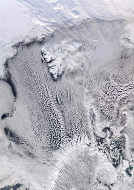
B Geerts et al., January 2021, DOE/SC-ARM-21-001

all cloud types (Remillard and Tselioudis 2015). The surface latent and sensible heat fluxes in CAOs may
be higher than anywhere else on Earth, often in excess of 500 W m-2 (Shapiro et al. 1987). Thus, even
though CAO events are transient, they may have a profound impact on circulations in the atmosphere,
where they may impact polar cyclogenesis (Terpstra and Spengler 2016), the intensity of baroclinic
disturbances, and the location of the mid-latitude storm track. CAO events also affect ocean circulations:
the heat loss they cause in the near-surface layers may be sufficiently strong in some areas for the surface
waters to become negatively buoyant, sink to depth and form deep ocean water (Dickson et al. 1996, Spall
and Pickart 2001). Changes in frequency and intensity of CAOs in a changing climate and changing arctic
sea ice extent thus may have profound feedbacks on the climate system, e.g., on polar cyclogenesis (Zahn
and von Storch 2010) and deep-water formation (Moore et al. 2015).

The depth, size, and linear/cellular organization of BLC are highly fetch-dependent and contingent on
synoptic conditions, in particular, surface wind speed and temperature, and stability of the layer above the
developing MBL. BLC involves interactions between surface fluxes, turbulence, clouds, and
precipitation, as well as radiative processes. While many field campaigns and related modeling studies
have explored the MBL in warmer climates, especially over subtropical oceans, numerical models (in
particular, regional climate models) are far less constrained by observations in CAOs at high latitudes.

To improve our understanding of BLC associated with CAO events, and to develop parameterizations
appropriate for climate models, observations are required to determine the environmental parameters that
control their microphysical and macrophysical properties, and thus ultimately to determine how they
change in response to global warming. Because low-level clouds are sensitive to sensible and latent heat
fluxes from the ocean surface, co-located observations of cloud and ocean properties are needed to
determine the ocean-atmosphere interactions affecting BLC. Aerosols are also believed to greatly
influence CAO low-level clouds. Although some studies have shown how CAO low-level clouds vary in
response to changes in the concentration and composition of aerosols (e.g., Lance et al. 2011, Jackson et
al. 2012), these prior campaigns have concentrated on measurements near Barrow, Alaska in coastal
regions, and have not had an adequate sample to determine how the aerosol effects vary with surface,
meteorological, and aerosol characteristics. Dedicated data collection focusing on a specific cloud system
that remains rather poorly documented will improve the representation of aerosol, clouds, radiation, and
precipitation processes in numerical weather prediction (NWP) models and in regional and global climate
models. CAOs also affect the climate system through oceanographic processes, in particular, by
modulating surface heat and momentum fluxes and deep-water formation.

This is the broad motivation for the COMBLE (Cold-air Outbreaks in the Marine Boundary Layer
Experiment) campaign, conducted successfully between 1 December 2019 and 31 May 2020 around the
Norwegian Sea, to focus on convective clouds in the MBL during CAOs, as illustrated in Figure 1.

 2
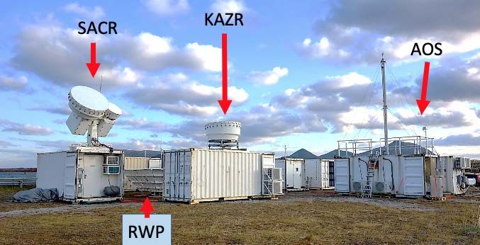
B Geerts et al., January 2021, DOE/SC-ARM-21-001

 Figure 1. Moderate Resolution Imaging Spectroradiometer (MODIS) visible image of a CAO event in
 the Norwegian Sea on 17 March 2019 (source: https://earthobservator.nasa.gov/).

 COMBLE data will improve the representation of aerosol particles, clouds, radiation, precipitation, and
 boundary-layer processes in regional and global climate models. These data are sorely needed since MBL
 clouds represent a significant challenge to regional and global climate models, especially in high-latitude
 regions, as they generally are sub-grid-scale and fall in the gray zone where boundary-layer processes and
 convection are tightly coupled and cannot be parameterized independently. Mutual benefits are expected
 because COMBLE will coincide with several related efforts, in particular, MOSAiC.

2.0 Notable Events or Highlights

 2.1 Instruments and Instrument Performance
 The ARM crew was able to maintain robust operations for all 6 months at the AMF1 site (called ANX in
 COMBLE) and at Bjørnøya (Bear Island, called S2 in COMBLE), notwithstanding the COVID-19
 pandemic. Met Norway assisted ARM in many aspects, ranging from site surveys to the operation of
 ARM instruments at Bjørnøya. The AMF1 instrument deployment at AMF1 is shown in Figure 2. Details

 3
B Geerts et al., January 2021, DOE/SC-ARM-21-001

of the instruments can be found at the ARM Data Center,
https://www.arm.gov/research/campaigns/amf2020comble

Radiosonde data were collected every 6 hours from the AMF1 site, and every 3 hours (during CAOs only)
from the ENAN site located in Andenes some 20 km to the NE (thanks to Met Norway personnel)
(Figure 3). In addition, Met Norway operated a volume-scanning C-band radar called Trolltinde some 14
km from the AMF1 site, on a ~300-m-high hill (Figure 3). These data are available in the ARM Data
Center.

Figure 2. Instruments at AMF1, located in Nordmela harbor, on Andøya, an island just off the northern
 Norwegian mainland (Figure 3).

 4
B Geerts et al., January 2021, DOE/SC-ARM-21-001

Figure 3. Terrain map surrounding the AMF1 site in COMBLE. The ENAN WMO sounding site is in
 the town of Andenes, at the northern tip of Andøya.

With the critical assistance of ARM technicians onsite, aerosol filter collections for subsequent
measurements of immersion freezing ice nucleating particle (INP) concentrations as a function of
temperature were made over periods of 6 to 74 hours (average 34 h and 42 m3 filtered), with periods
tailored to integrate CAO or flanking periods of non-CAO air (DeMott and Hill 2020, in preparation).
Open-faced filters were sampled at a height of 4 m AGL on the Aerosol Observing System (AOS) trailer
(6 m below its inlet, visible under a rain “hat” in Figure 2). A total of 68 filters (4 blanks) were collected
over the COMBLE deployment, stored at -20°C following sampling, and returned frozen in a dry nitrogen
shipper for processing at Colorado State University (CSU) at the end of the campaign. Processing of
re-suspended particles in the CSU ice spectrometer provided INP concentrations from 0 to -29°C for
63 sample periods. Additional processes to identify INP compositional contributions as biological,
organic, and inorganic were performed on roughly 40% of the samples. The data set is described in
DeMott and Hill (2020, in preparation), and data have been submitted to the ARM Data Center.

Three instrument issues occurred at the AMF1 site:
 • Micropulse lidar (MPL) – transferred to MOSAiC early in campaign
 • Humidified tandem differential mobility analyzer (HTDMA) and aerosol chemical speciation monitor
 (ACSM) – down for much of campaign
 • Radar wind profiler (RWP) – down for several weeks.

 5
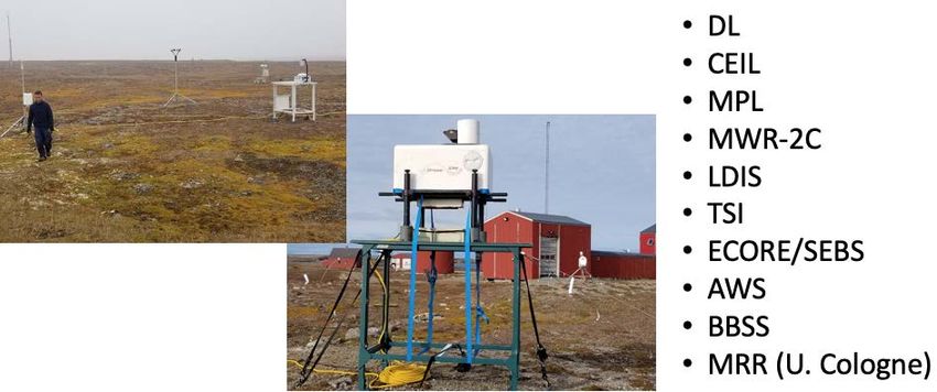
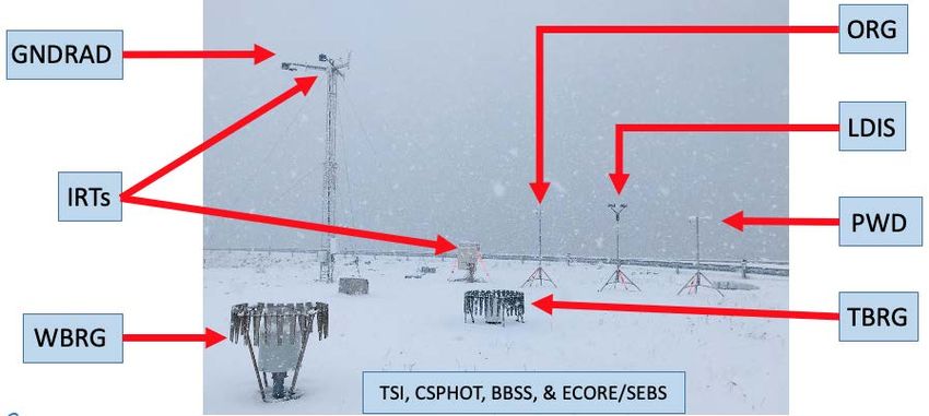
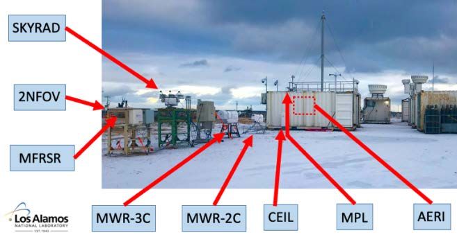
B Geerts et al., January 2021, DOE/SC-ARM-21-001

The AMF1 instrument deployment at Bjørnøya is shown in Figure 4. In addition to the ARM data, there
are 3-hourly radiosondes by Met Norway (World Meteorological Organization [WMO] site code: ENBJ)
during CAOs only, although some of these did not materialize for a variety of reasons (technical and
personnel-related). The University of Cologne collected MicroRain Radar (MRR) data during COMBLE
from Bjørnøya, and these data are planned to be in the ARM Data Center soon (contact: Kerstin Ebell
kebell@meteo.uni-koeln.de).

 Figure 4. Instruments at the site of the Met Norway station on the north side of Bjørnøya.

Two instrument issues occurred at Bjørnøya:
 • MPL became encrusted in snow and ice; data loss for a few weeks, until it was moved.
 • Microwave radiometer−2-channel (MWR−2C) had a broken component, which was repaired,
 notwithstanding the remote location.

2.2 Weather Conditions
A cumulative total of 23 days of CAO conditions was observed at the AMF1 site during COMBLE, with
an average M value (a measure of thermal instability driven by surface heat fluxes) of 3.4 K. Here, CAO
conditions are defined as:
1. M>0, where ≡ − 850 ℎ , and SST is the sea surface temperature about 10 km offshore the
 AMF1 site
2. Ka-band ARM Zenith Radar (KAZR) first echo top below 5.0 km (not enforced for now, because of
 frequent seeder-feeder situations)
3. surface wind speed >10 kts
4. surface wind direction between 250 and 30 degrees
5. continuity: short gaps (
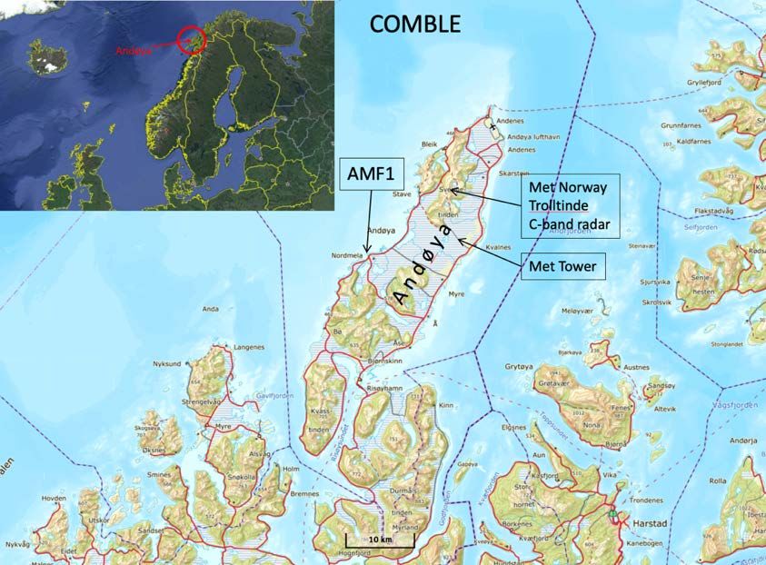
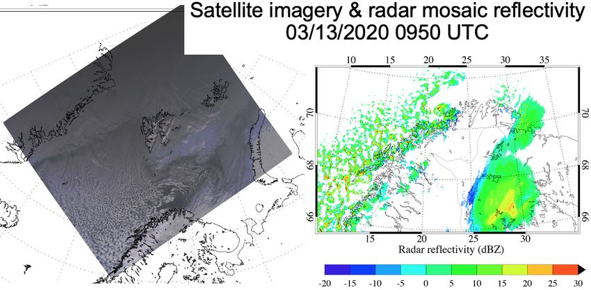
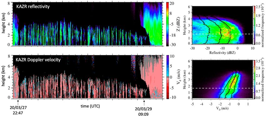
B Geerts et al., January 2021, DOE/SC-ARM-21-001

The better CAO cases are listed in Table 1. These cases stand out in terms of their persistently high
M value, their synoptic signature (with trajectories originating over the arctic sea ice), and their duration.
Also, in all three cases, winds at ANX were rather strong, and the wind direction close to normal to the
shore of Andoya.

 Table 1. The three best CAO cases at the AMF1 site. M is defined above.
 Mean Wind
 Start time End time Duration Magnitude Mean Wind
 (yy/mm/dd zz) (yy/mm/dd zz) (minutes) Mean M [K] [m/s] Direction [°]

 20/02/04 15:47 20/02/06 13:04 2718 7.2 7.7 308
 20/03/27 22:47 20/03/29 09:09 2063 6.6 8.0 314
 20/03/12 18:30 20/03/14 02:09 1900 7.8 7.6 336

Sample satellite and radar images of two of the three cases listed in Table 1 is shown in Figure 5. Both
cases reveal air trajectories originating at the ice edge in the northern Fram Strait. No MODIS imagery is
available for the third case in early February because the Norwegian Sea was still largely in the polar
night during Aqua/Aura overpasses.

The vertical structure of the CAO cloud regime is illustrated in Figure 6, for the 27-29 March 2020 case.
Clouds clearly are convective, and they are remarkably deep, up to 4.5 km deep, much deeper than the
traditionally defined MBL. Towards the end of this CAO, upper-level warm-frontal clouds overrun the
shallow cold-airmass, gradually deepening and stifling the CAO.

 7
B Geerts et al., January 2021, DOE/SC-ARM-21-001

Figure 5. (left) MODIS visible imagery (data source: https://earthobservatory.nasa.gov/) and (right)
 Met Norway radar mosaic (data source: https://thredds.met.no) for two of the three better
 CAOs in COMBLE.

Figure 6. (left) KAZR reflectivity and Doppler velocity profiles for the CAO of 27-29 March 2020.
 (right) Corresponding CFADs (contoured frequency by altitude diagrams). The solid black
 lines are the 25/50/75 percentiles, and the dotted line is the average.

The red periods in Figure 7 show all CAO periods, as defined above. (Data were collected continuously,
so non-CAO periods can be studied as well.) CAO conditions were more common on Bjørnøya, and the
thermal instability higher, as expected from climatology. We are waiting for the interpsonde value-added
produce (VAP) to finalize the CAO periods on Bjørnøya.

 8
B Geerts et al., January 2021, DOE/SC-ARM-21-001

 Figure 7. CAO periods at the AMF1 site during the COMBLE campaign, between 1 December 2019
 and 31 May 2020.

3.0 Some Preliminary Results
 Altogether, COMBLE was a great success. A wide range of thermal instability, wind speed, cloud top
 height, and precipitation intensities were observed at both sites during CAOs in COMBLE. Figures 7-14
 show environmental conditions and basic cloud properties during the CAO periods at the AMF1 site. The
 mean M value was 3.9 K at the AMF1 site (Figure 8). The surface winds were between westerly and
 northerly, mainly ~320° (NW), which is roughly normal to the Andøya coastline (Figure 9). The surface
 temperature generally was between 0-5°C (Figure 11), and the CAO clouds generally produced light
 precipitation (Figure 15).

 Some of these results are preliminary, for instance, a better definition of MBL depth is possible
 (Figure 12).

 We are planning to do the same analysis for Bjørnøya, once we can define CAO conditions there (for
 which we need interpsonde data. The AMF1 site was located at rather great fetch (about 1000-1200 km)

 9
B Geerts et al., January 2021, DOE/SC-ARM-21-001

from the arctic ice edge, at Nordmela harbor, on the island of Andøya just off the coast of northern
Scandinavia). The Bear Island site was located some 500 km closer to the ice edge. In March 2020, the
marginal ice zone briefly reached this island, as arctic ice was advected from the east side of Svalbard.

Any study of the CAO cloud regime at the AMF1 site should take into account the possible influence of
downwind topography. Within a few km, terrain ~300 m high is present, on the island of Andøya. Further
downwind, over a distance of ~50 km, the Scandinavian highlands ~1200 m high are present with deep
fjords intersecting the foreland (Figure 3). This terrain impacts synoptic, mesoscale, and local
circulations, and thus cloud and precipitation.

This influence is suggested in the KAZR reflectivity profiles. In many cases precipitation fell
continuously from upper cloud layers into the boundary-layer (BL) clouds: therefore the BL cloud top
height could not be readily defined. This appears more prevalent in COMBLE than at ARM’s North
Slope of Alaska (NSA) site, for instance, because the immediate hinterland of the AMF1 site in
COMBLE is mountainous (versus flat at the NSA site). Upslope flow over this downwind terrain
presumably caused ascent of free-tropospheric layers, resulting in sometimes deep precipitation profiles
above the AMF1 site, hiding the BL clouds. We plan to use KAZR Doppler velocity and spectral width
data to identify these cases of upper-level clouds feeding shallow clouds.

 Figure 8. Distribution of M values, at the AMF1 site during CAO periods identified in Figure 7.

 10
B Geerts et al., January 2021, DOE/SC-ARM-21-001

Figure 9. Surface wind direction, at the AMF1 site during CAO periods identified in Figure 7.

 Figure 10. Surface wind speed, at the AMF1 site during CAO periods identified in Figure 7.

 11
B Geerts et al., January 2021, DOE/SC-ARM-21-001

 Figure 11. Surface temperature, at the AMF1 site during CAO periods identified in Figure 7.

Figure 12. Best-estimate boundary-layer (mixed-layer) depth, at the AMF1 site during CAO periods
 identified in Figure 7.

 12
B Geerts et al., January 2021, DOE/SC-ARM-21-001

Figure 13. Cloud base estimated from ceilometer and/or micropulse lidar, at the AMF1 site during CAO
 periods identified in Figure 7.

Figure 14. Best-estimate echo top height of lowest cloud layer, at the AMF1 site during CAO periods
 identified in Figure 7.

 13
B Geerts et al., January 2021, DOE/SC-ARM-21-001

 Figure 15. Precipitation rate, at the AMF1 site during CAO periods identified in Figure 7.

4.0 Public Outreach
 The COMBLE campaign was conducted at a remote location, with no principal investigator (PI) presence
 at the site, hence there was no open house or other outreach to local schools or universities. There were
 several news coverages and blogs about COMBLE, archived at the ARM website:
 https://www.arm.gov/news-events/search?q=comble

5.0 COMBLE Publications

 5.1 Journal Article Manuscripts
 At this time, no journal articles focused on COMBLE have been published, but several are in preparation.

 5.2 Meeting Abstracts/Presentations/Posters
 Dedicated sessions on COMBLE were held at the ARM/Atmospheric System Research (ASR) Joint PI
 meetings in 2019 and 2020, as well as presentations focused on or mentioning COMBLE at the 2020
 American Geophysical Union Fall meeting, including Geerts et al. (2020).

6.0 References
 Arctic Climate Impact Assessment. 2005. Arctic Climate Impact Assessment: Scientific Report.
 Cambridge University Press, Cambridge, United Kingdom, and New York, New York, USA.

 14
B Geerts et al., January 2021, DOE/SC-ARM-21-001

DeMott, PJ, and TCJ Hill. 2020. COMBLE ARM Mobile Facility (AMF) Measurements of Ice
Nucleating Particles Final Campaign Report (in preparation as ARM user facility publication, December
2020).

Dickson, R, J Lazier, J Meincke, P Rhines, and J Swift. 1996. “Long-term coordinated changes in the
convective activity of the North Atlantic.” Progress in Oceanography 38(3): 241–295,
https://doi.org/10.1016/ S0079-6611(97)00002-5

Geerts, B, et al. 2020. Microphysics and mesoscale dynamics of marine boundary-layer clouds in cold air
over open water. Paper A020-06, American Geophysical Union Fall Meeting (virtual).

Hartmann, DL, B-ME Ockert, and ML Michelsen. 1992. “The effect of cloud type on earth’s energy
balance: Global analysis.” Journal of Climate 5(11): 1281–1304, https://doi.org/10.1175/1520-
0442(1992)0052.0.CO;2

Inoue, J, J Liu, JO Pinto, and JA Curry. 2006: “Intercomparison of Arctic Regional Climate Models:
Modeling Clouds and Radiation for SHEBA in May 1998.” Journal of Climate 19(17): 4167−4178,
https://doi.org/10.1175/JCL13854.1

Intergovernmental Panel on Climate Change. 2013. Climate Change 2013: The Physical Science Basis.
Cambridge University Press, Cambridge, United Kingdom and New York, New York, USA.

Jackson, RC, GM McFarquhar, AV Korolev, ME Earle, PSK Liu, RP Lawson, S Brooks, M Wolde,
A Laskin, and M Freer. 2012. “The dependence of ice microphysics on aerosol concentration in arctic
mixed-phase stratus clouds during ISDAC and M-PACE.” Journal of Geophysical Research –
Atmospheres 117(D15): D15207, https://doi.org/10.1029/2012JD017668

Kay, JE, and A Gettelman. 2009. “Cloud influence on and response to seasonal Arctic sea ice loss.”
Journal of Geophysical Research – Atmospheres 114(D18): D18204,
https://doi.org/10.1029/2009JD011773

Lance, S, MD Shupe, G Feingold, CA Brock, J Cozic, JS Holloway, RH Moore, A Nenes, JP Schwarz,
JR Spackman, KD Froyd, DM Murphy, J Brioude, OR Cooper, A Stohl, and JF Burkhart. 2011. “Cloud
condensation nuclei as a modulator of ice processes in Arctic mixed-phase clouds.” Atmospheric
Chemistry and Physics 11(15): 8003−8015, https://doi.org/10.5194/acpd-11-8003-2011

Moore, G, K Våge, RS Pickart, and IA Renfrew. 2015. “Decreasing intensity of open-ocean convection in
the Greenland and Iceland seas.” Nature Climate Change 5: 877–882,
https://doi.org/10.1038/nclimate2688

Rémillard, J, and G Tselioudis. 2015. “Cloud Regime Variability over the Azores and its Application to
Climate Model Evaluation.” Journal of Climate 28(24): 9707–9720, https://doi.org/10.1175/JCLI-D-15-
0066.1

Shapiro, MA, LS Fedor, and T Hampel. 1987. “Research aircraft measurements of a polar low over the
Norwegian Sea.” Tellus A: Dynamic Meteorology and Oceanography 39(4): 272–306,
https://doi.org/10.1111/j.1600-0870.1987.tb00309.x

 15
B Geerts et al., January 2021, DOE/SC-ARM-21-001

Solomon, A, G Feingold, and MD Shupe. 2015. “The role of ice nuclei recycling in the maintenance of
cloud ice in Arctic mixed-phase stratocumulus.” Atmospheric Chemistry and Physics Discussions 15(18):
11727−11761, https://doi.org/10.5194/acpd-15-11727-2015

Spall, MA, and RS Pickart. 2001. “Where does dense water sink? A subpolar gyre example.” Journal of
Physical Oceanography 31(3): 810–826, https://doi.org/10.1175/1520-
0485(2001)0312.0.CO;2

Terpstra, A, and T Spengler. 2016. Influence of surface fluxes on polar low development: Idealised
simulations. Presented at the European Geophysical Union General Assembly, 17-22 April, 2016, Vienna,
Austria, p.11414.

Vavrus, S. 2004. “The Impact of Cloud Feedbacks on Arctic Climate under Greenhouse Forcing.”
Journal of Climate 17(3): 603–615, https://doi.org/10.1175/1520-
0442(2004)0172.0.CO;2

Zahn, M, and H von Storch. 2010. “Decreased frequency of North Atlantic polar lows associated with
future climate warming.” Nature 467: 309–312, https://doi.org/10.1038/nature09388

 16
You can also read