R enyi's spectra of urban form for different modalities of input data
←
→
Page content transcription
If your browser does not render page correctly, please read the page content below
Rényi’s spectra of urban form for different modalities of
                                                                          input data
                                                        Mahmoud Saeedimoghaddama , T. F. Stepinskia,∗, Anna Dmowskaa
arXiv:2007.07410v1 [physics.soc-ph] 15 Jul 2020

                                                          a
                                                              Space Informatics Lab, University of Cincinnati, Cincinnati, OH, USA.

                                                  Abstract

                                                  Morphologies of urban patterns display multifractal scaling. However, what
                                                  data should be used to represent an urban pattern and its scaling? Here,
                                                  we calculated Renyi’s generalized dimensions (RGD) spectra using data cor-
                                                  responding to different urban modalities including urban land cover, urban
                                                  impervious surface, population density, and street intersection points. All
                                                  data are circa 2010 and we calculated their RGD spectra in six urbanized
                                                  areas located across the United States. We calculated the RGD spectra
                                                  by using Hill’s numbers rather than statistical moments which leads to a
                                                  clear interpretation of generalized dimensions and to spatial visualization
                                                  of pattern’s multifractality. The results show that patterns of different ur-
                                                  ban modalities in a given urbanized area are characterized by different RGD
                                                  spectra and thus have different morphologies. In our six examples, we found
                                                  that morphologies of patterns of land cover and impervious surface tend to
                                                  be monofractal, patterns of street intersection points tend to be moderately
                                                  multifractal, and patterns of population density tend to be strongly multi-

                                                    ∗
                                                     Corresponding Author
                                                     Email addresses: saeedimd@mail.uc.edu (Mahmoud Saeedimoghaddam),
                                                  stepintz@uc.edu (T. F. Stepinski), dmowska83@gmail.com (Anna Dmowska)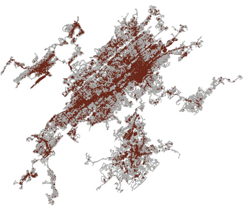
fractal. Spatial visualization supporting this numerical finding is provided.
Thus, when studying the multifractality of urban morphology, it is impor-
tant to choose a modality that is appropriate to the goal of the investigation.
Urban areas may have similar morphologies on the basis of one modality but
dissimilar on the basis of another. We have found that two out of our six
urban areas have similar morphologies on the basis of all four modalities.
Keywords: Fractals, Multifractal scaling, Urban form, Hill’s numbers,
Visualization

1. Introduction

   When observing urban agglomerations in high-resolution satellite images
it is clear that, while specific details vary, their spatial forms are always
heterogeneous and hierarchically self-similar [16; 7; 32] with areas of a very
low level of urbanization interwoven into areas of a very high level of urban-
ization. Large number of previous studies showed that urban forms can be
described in terms of fractal geometry [6; 8; 13; 36; 10].
   Closer examination [3; 5] reveals that urban forms are best quantified by
a multifractal rather than fractal (monofractal) description. Let assume that
the urban system consists of a set of points or pixels each representing a sin-
gle urban element. If any portion of such set is statistically identical to the
original set (statistical self-similarity), the set is fractal, and the urban form
has a fractal form. In a fractal all the moments of the probability distribu-
tion function scale in the same way so the fractal can be characterized by a
single number - a fractal dimension D - which refers to the invariance of the
probability distribution function with the change of spatial scale. However,

                                        2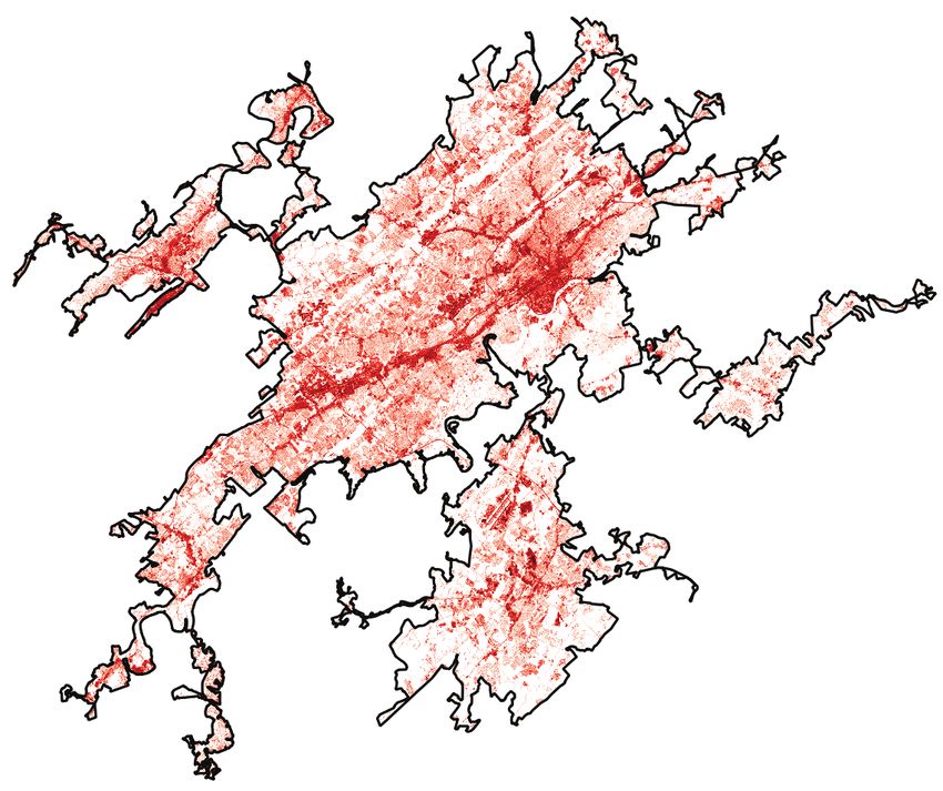
for the majority of urban systems, the moments of probability distribution
function do not scale in the same way and the entire spectrum of numbers –
generalized fractal dimensions – is needed to characterize the urban form [17].
In such case, the urban form is multifractal. The name multifractal reflects
the fact that sparser and denser parts of the urban system have different
scaling behaviors.
   We can divide the literature on the multifractal description of urban form
on the basis of the type of data used. Different urban forms may be revealed
by analyzing different types of data. Possible data modes include classified
satellite multispectral images, population grids, street intersections datasets,
and night-time lights images. Multispectral satellite images of an urban area
can be classified into land cover/land use (LCLU) raster maps as well as used
to obtain raster maps of impervious surfaces. LCLU map is converted into a
binary map (urban/non-urban pixels); from that binary map, a multifractal
spectrum characterizing urban form is calculated [23; 10; 34]. A map of
urban impervious surface (UIS) is a numerical raster where each pixel has a
value between 0 and 1 indicating a share of impervious cover within a pixel.
Multifractal characterizations of UIS patterns were performed by Nie and
Liu [25] and Man et al. [20]. Imagery data provides information about the
distribution of man-made constructions, consequently, multifractal analysis
of imagery data pertains to the spatial form of a built-up area.
   Population data comes from national censuses and is available in the form
of aggregated units (shapefile data), however, gridded population datasets,
more useful for multifractal analysis, have been derived from original census
data [35; 14]. Most of the multifractal analyzes of population distribution

                                       3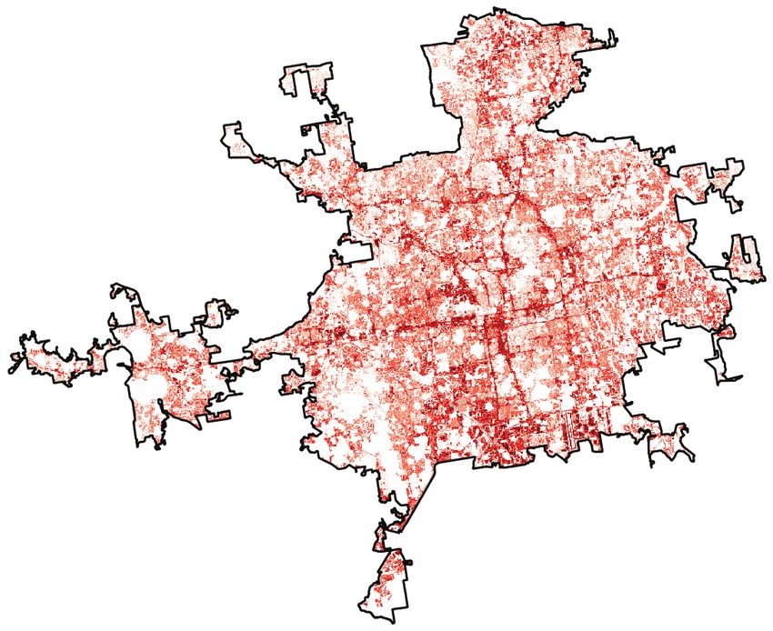
were conducted for entire countries rather than for urban areas. Adjali and
Appleby [1] derived multifractal spectra for population distribution for ten
different countries. Mannersalo et al. [21] applied multifractal analysis to the
population distribution of Finland, Semecurbe et al. [33] performed a similar
analysis for France, and VegaOrozco et al. [37] for Switzerland. Only Chen
and Feng [9] performed multifractal analysis for the population distribution
of a single urban area – Hangzhou, China. Population data provides informa-
tion about the distribution of people and thus its multifractal analysis may
reveal a different urban structure than the analysis applied to a built-up area.
   Recently, street intersection points (SIP) data was used for multifractal
analysis of urban form [22]. SIP data provides a good proxy for urban form [4;
24; 29], especially for studying the long-term temporal evolution of the form,
because of the availability of detailed historical maps of road intersections.
Such data provides a modality of urban form which is different from those
provided by either population data or built-up area data. Finally, Ozik et al.
[26] performed a multifractal analysis of the worldwide distribution of urban
areas using night-time lights satellite images. However, the resolution of such
data is too coarse to be used for an analysis of a single urban area.
   The contribution of this paper is to compare spatial forms of an urban area
as indicated by multifractal analysis of different modes of form-indicating
data. Do all data modes indicate the same form or are there significant dif-
ferences in an urban form depending on what data is used? We have selected
six urbanized areas (UAs) throughout the United States. For each UA we
calculated the Renyi’s generalized dimensions (RGD) spectra of four spatial
patterns: land cover (LCLU), percentage of impervious cover (UIS), pop-

                                       4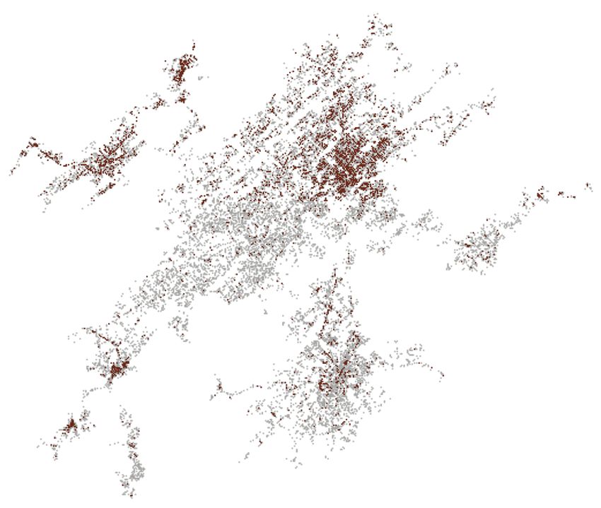
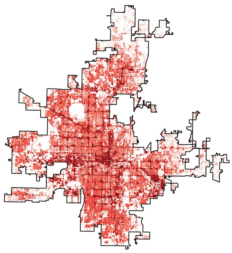
population (POP)             land cover (LCLU)       impervious surface (UIS) street intersections (SIP)
     Knoxville (KNX)
     Oklahoma City (OKC)
      Orlando (ORL)

                           lowest             highest                             lowest                highest
                                                          non-urban urban
                                                                                                                  street intersection point
                                    density                                                percentage

Figure 1: Spatial depiction of four data modes in three out of six urbanized areas analyzed
in this study.

ulation density (POP), and street intersection points (SIP). An additional
contribution of this paper is a description of RGD spectra in terms of Hill’s
numbers [18] instead of statistical moments of probability function charac-
terizing a pattern. As a result, the meaning of generalized dimensions is
more transparent. In addition, we can visualize the multifractal structure of
spatial patterns as maps of Hill’s numbers.

2. Data

    We analyze six UAs in their 2010 boundaries, Knoxville, TN (KNX) Ok-
lahoma City, OK (OKC), Orlando, FL (ORL), Philadelphia, PA (PHL),
Phoenix, AZ (PHX), and Portland, OR (POR). The US Census Bureau de-

                                                                            5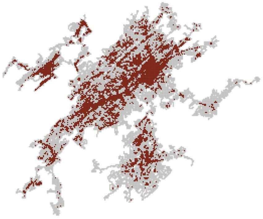
fines an urbanized area as a densely developed territory with a population
over 50,000 that encompass residential, commercial, and other non-residential
urban land uses. A UA usually serves as the core of a larger metropolitan
statistical area. Within a boundary of each UA, we analyze spatial patterns
of LCLU, UIS, POP, and SIP. All data sets are circa 2010.
   LCLU and UIS data are from the National Land Cover Database (https://www.mrlc.gov/).
We use the 2011 edition of LCLU and UIS as the 2010 edition is not available.
The LCLU data provides nationwide data on the land cover at a 30m/cell
resolution with a 16-class legend based on a modified Anderson Level II
classification system. We have reclassified the original LCLU data to only
two categories, urban, consisting of three classes (developed low intensity,
developed medium intensity, developed high intensity) and non-urban (the
remaining 13 classes). In the box-counting method of multifractal analysis, a
LCLU “mass” of a box is the number of urban cells. The UIS data represent
urban impervious surfaces as a share (from 0 to 1) of a developed surface
over every 30m cell in the United States. In the box-counting method of
multifractal analysis, a UIS “mass” of a box is the sum of urban impervious
surfaces shares for all cells in a box.
   The POP data represents population density. It is in the form of 30m/cell
grid where each cell has a number of people per cell (the value of the cell could
be a fraction). The POP data is available from SocScape (http://sil.uc.edu)
and is the result of dasymetric modeling of 2010 US Census Bureau block-
level aggregated data [14; 15]. In the box-counting method of multifractal
analysis, a POP “mass” of a box is the sum of all people in cells present in
a box (the total number of people in a box). The SIP data starts with 2010

                                          6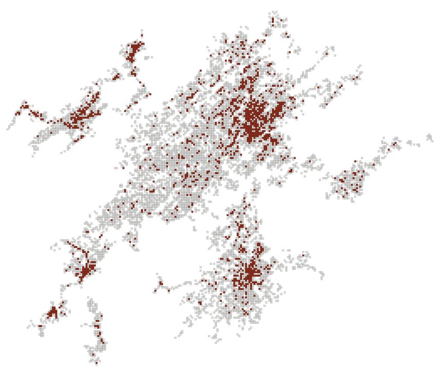
street networks provided by the US Census Bureau (https://www.census.
gov/cgi-bin/geo/shapefiles/index.php?year=2010&layergroup=Roads).
For fixing the topological errors of the street networks we used ArcMap soft-
ware. “Line intersections” tool in QGIS software has been employed to ex-
tract the junctions (intersections) from the networks. Whereas LCLU, UIS,
and POP are grid data, SIP is a point data. In the box-counting method of
multifractal analysis, a SIP “mass” of a box is the sum of street intersection
points in a box.
   Fig. 1 shows patterns of POP, LCLU, UIS, and SIP for three out of six
UAs analyzed in the paper. The cells are colored according to respective
legends. Whether morphologies of different modalities of urban data are
similar or dissimilar and whether the patterns are mono- or multi-fractal is
not readily apparent from patterns as shown in Fig. 1, but it will become
apparent from their RGD spectra.

3. Methods

   Urban system (for example, an UA) consists of discrete urban elements.
In this paper, urban elements are either street intersection points or pixels in
maps of land cover, percentage of impervious area, and population density.
The spatial pattern of urban elements forms an urban morphology that we
want to quantify. We are not interested in an overall layout of an urban area
but rather in the statistical properties of its hierarchical structure. For this
purpose, we are using multifractal analysis.
   We discuss multifractal analysis through the prism of box-counting method
[11]. Box counting method is based on a series of grids with different cell

                                       7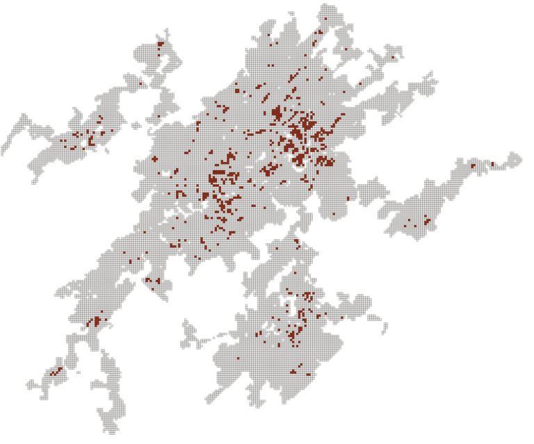
(box) sizes; each grid covers the entire pattern of urban elements. For a grid
with given box size, (), a mass (see the previous section) of each box is
calculated and stored in the originating box thus transforming a grid to a
numerical array. Dividing the mass of each box by the total mass of all ur-
ban elements in a region yields a probability distribution {pi } = {p1 , . . . pn },
where n is the number of nonempty boxes. Note that both, probability dis-
tribution and the value of n depend on the grid size , dependence that, for
a moment, is not reflected in the notation to make the text more lucid. The
probability distribution of urban pattern, like all probability distributions,
may be characterized by its statistical moments,
                                        X
                                 Mq =        pi ()q                            (1)
                                         i

where ∞ ≤ q ≤ ∞ is called a moment order. The multifractal analysis
consists of determining whether statistical moments of -series of {pi } have
power-law scaling with . If all moments have identical power-low scaling the
urban morphology is fractal (monofractal), if they have power-law scaling
but with different exponents the urban morphology is multifractal, and if
they don’t have the power-law scaling the urban morphology is nonfractal.
Assuming that the urban structure is either monofractal or multifractal, the
results of the multifractal analysis is summarized by the Renyi’s generalized
dimensions (RGD) spectrum [30].
   Most descriptions of the RGD in the urban context [22; 31; 9] are in term
of Mq , however, in our opinion, description of RGD in terms of Hill’s numbers
[18] provides more connection to the data and enables spatial visualization
of urban structure in terms of RGD. The connection between moments Mq

                                         8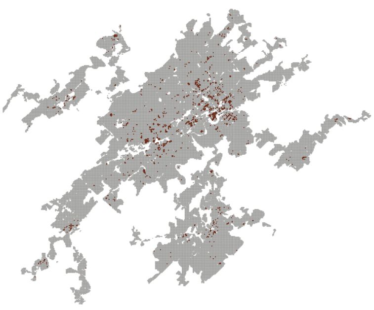
and Hill’s numbers Nq is as follows,
Mq1/(1−q)
if q 6= 1
Nq = (2)
a− ni=1 pi log pi
P
if q = 1
where a is the base of the logarithm used in the equation.
To better understand the meaning of Nq note that Mq can also be written
as i wi pq−1
P
i , where wi = pi but is interpreted here as a weight, so Mq could
be interpreted as a weighted mean of the (q − 1)th powers of the relative
frequencies of urban elements in nonempty boxes and denoted by hpq−1 i.
1/(q−1)
Then, hpiq = hpq−1
i i is the generalized average probability (average
relative frequency of urban elements per box). It is called “generalized”
because its value depends on the way the average is defined which, in turn,
depends on the value of q.
The reciprocal of hpiq is the Hill’s number Nq . Thus, Nq is a number of
equally abundant boxes to have average probability the same as the gener-
alized average probability of all boxes. For this reason Nq may be referred
to as an effective number of boxes. As q decreases from ∞ to −∞, hpiq
decreases from max pi to min pi and Nq increases from 1/ max pi to 1/ min pi .
For q = 0, hpiq = 1/n and Nq = n.
Nq is a measure of diversity or disparity of values in the distribution.
Small values of Nq indicate distributions restricted to a few high-density
boxes, whereas large values of Nq indicate distributions spread over all or
the majority of the boxes. For q ≥ 0, the range of values of Nq is between
n (when q = 0) and 1 (when q = ∞ and there is only one box with the
maximum value of probability). For q < 0, the hpq−1 i is very small and,
consequently Nq > n.
9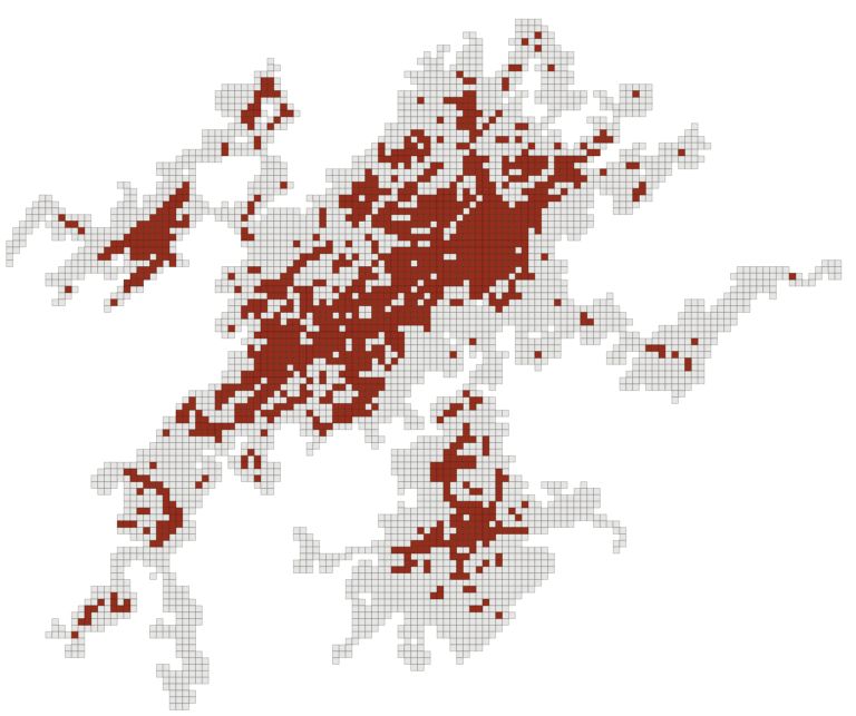
Renyi’s generalized entropy Hq [30] is related to Nq as follows,
log Nq ()
if q 6= 1
Hq () = Xn (3)
− pi () log pi () if q = 1
i=1
where we now explicitly show dependence on spatial scale . The generalized
dimension, Dq , is calculated as Dq = − lim→0 Hq / log , or, in terms of Nq ,
−lim loglog
Nq ()
if q 6= 1
→0
Dq = (4)
Pn
−lim − i=1 pi () log pi () if q = 1
→0 log
Thus, generalized dimensions are the rates of change of effective number
of boxes with scale, Nq () ∼ −Dq . Because N0 () = n(), D0 is a fractal
dimension. Other Dq are rates of change of a number of boxes in density-
limited subsets of the urban area. The function Dq (q) is referred to as the
RGD spectrum; it provides a unique description of an urban pattern.
The importance of expressing generalized dimensions in terms of Hill’s
numbers is that it gives a transparent meaning to generalized dimensions.
In addition, for nonnegative orders, the -series of Nq corresponds to nested
subsets Sq of an -sized grid, such that S∞ ⊂ · · · ⊂ Sk+1 ⊂ Sk ⊂ · · · ⊂ S1 ⊂
S0 . The S∞ consists of N∞ densest boxes (could be as little as one box),
Sk consists of Nk densest boxes (which include all boxes in Sk+1 ), and S0
consists of all nonempty boxes in the -sized grid. The -series of maps of
these subsets forms a spatial visualization of multifractality of urban pattern.
102.0 2.0 2.0
1.8 1.8 1.8
1.6 1.6 1.6
Dq
Dq
Dq
1.4 1.4 1.4
1.2 1.2 1.2
Knoxville (KNX) Oklahoma City (OKC) Orlando (ORL)
1.0 1.0 1.0
- 20 - 10 0 10 20 - 20 - 10 0 10 20 - 20 - 10 0 10 20
q q q
2.0 2.0 2.0
1.8 1.8 1.8
1.6 1.6 1.6
Dq
POP
Dq
Dq
1.4 1.4 1.4 SIP
UIS
LCLU
1.2 1.2 1.2
Philadelphia (PHL) Phoenix (PHX) Portland (POR)
1.0 1.0 1.0
- 20 - 10 0 10 20 - 20 - 10 0 10 20 - 20 - 10 0 10 20
q q q
Figure 2: RGD spectra of patterns of LCLU (orange), UIS (green), POP (red) and SIP
(blue) in six urban areas analyzed in this study.
4. Empirical results
For each UA, we calculated RGD spectra of 2010 SIP pattern, 2010 POP
pattern, 2011 UIS pattern, and 2011 urban LCLU pattern. To calculate
the RGD spectrum for each dataset, we utilized the globally normalized [2]
“enlarged box-counting” method [27] with a dyadic sequence of the box sizes
. We calculate values of Dq for q between -20 and 20 in step of 1, but only
keep the values fulfilling the following criteria, (1) the resultant value is in
the range 0 ≤ Dq ≤ 2, (2) R2 ≥ 0.9 in the regression estimation of linear fit
necessary to translate box counts into an estimate of Dq [22].
Fig. 2 shows the calculated RGD spectra, RGD spectra of SIP patterns
are shown in blue, RGD spectra of POP patterns are shown in red, RGD
spectra of LCLU are shown in orange, and RGD spectra of UIS patterns are
shown in green. The main result is that the multifractality of an urban form
11depends on the mode of the data used.
Table 1: Indices of multifractality ∆ and ∆0 (slanted font)
data KNX OKC ORL PHL PHX POR
LCLU 0.3 0.15 0.32 0.17 0.14 0.16
0.07 0.06 0.04 0.02 0.05 0.04
UIS – – – 0.13 – –
0.09 0.18 0.22 0.08 0.14 0.13
POP – – – – – –
0.69 0.70 0.73 0.55 0.70 0.46
SIP 0.67 0.56 0.53 0.59 0.56 0.53
0.28 0.21 0.15 0.26 0.23 0.18
To measure the degree of multifractality we introduce two indices, ∆ and
∆0 . First, ∆ = max Dq − min Dq , it applies only to patterns where max Dq
corresponds to a negative value of q. As we can see from Fig. 2 in many
cases the RGD spectrum does not extend to negative values of q due to an
insufficient number of data and/or the breakup of the fractal character of
the pattern in a sparse portion of an urban area. Recall from the previous
section that the right part of the RGD spectrum (between q = ∞ and q = 0)
represents an accumulation of the effective number of boxes Nq from those
representing the densest part (q = ∞) to all boxes (q = 0). The left part
of the RGD spectrum (between q = −∞ and q = 0) also represents an
accumulation of effective number of boxes Nq from those representing the
sparsest part (q = −∞) to all boxes (q = 0).
Thus, if max Dq corresponds to the negative value of q, ∆ represents a
difference in scaling exponents of the sparsest and the densest parts of an
urban area. However, for patterns where max Dq = D0 such interpretation of
12∆ thus not hold. In such cases we define ∆0 = D0 − min Dq that represents
a difference in scaling exponents of the entire pattern and its densest part.
Note that ∆0 can also be defined for patterns that permit calculations of
Dq for negative values of q. Table 1 lists values of ∆ and ∆0 (slanted font).
Table 1 reveals that, in all six UAs, RGD spectra for patterns of POP cannot
be extended to negative values of q. RGD spectra for patterns of UIS cannot
be extended to negative values of q in five out of six urban areas.
In all six UAs values of ∆0 are small for patterns of LCLU. For such
patterns values of ∆ are also small with the exception of KNX and ORL.
Thus, with possible exception of their sparsest parts, patterns of LCLU are
monofractal. This is in agreement with the results of multifractal analy-
sis [10] of LCLU in Beijing, China. RGD spectra of patterns of UIS are
restricted mostly to nonnegative values of q (the single exception is Philadel-
phia). Small values of ∆0 indicate that these patterns tent to be only weakly
multifractal; the urban area of Orlando is an exception. This is in qualitative
agreement with the results of multifractal analyzes [25; 20] for patterns of
UIS in Shanghai and Xiamen, China, respectively
Patterns of POP have RGD spectra restricted to nonnegative values of
q. However, they are all strongly multifractal as indicated by large values
of ∆0 . Previous multifractal analysis of POP for urban area of Hangzhou
City, China [9] also found strong multifractality. Unlike in our study, these
authors calculated values of Dq for negative values of q with large absolute
values. This resulted in values of Dq as high as 3.5 which is not interpretable
in a 2D geometry. Restricting their results to Dq ≤ 2 eliminates values of Dq
for negative values of q and makes their result very similar to ours.
13Finally, for patterns of SIP, their RGD spectra extend to negative values
of q so values of both, ∆ and ∆0 can be calculated. Values of ∆ are large
indicating strong multifractality. However, the values of ∆0 are significantly
smaller, so there is a large difference in scaling exponents between sparsest
and densest parts of the SIP pattern, but a large part of this difference is
due to high scaling exponents for the sparsest parts of that pattern. Murcio
et al. [22] performed multifractal analysis of SIP for London as bounded
by an external boundary (the green zone) at different years starting from
1786 and ending in 2010. Qualitatively their results are in agreement with
ours inasmuch as they indicate strong multifractality for earlier years, and
their RGD spectra extend to negative values of q. However, their values of
Dq , for positive values q, are, in general, larger than ours indicating that
London, even in the past, had more space-filling network of streets than the
six present-day American cities analyzed in this paper.
5. Visualizing multifractal structure
Recall that expressing generalized dimensions in terms of Hill’s numbers
allows spatial visualization of the urban area’s multifractal structure. We
demonstrate such visualization for patterns of UIS, SIP, and POP in KNX.
Fractal dimensions (values of D0 ) for these three patterns are 1.71, 1.52,
and 1.74, respectively. Values of D10 , which can be interpreted as a fractal
dimension of pattern consisting of only denser part of the urban area, are
1.64, 1.30, and 1.12, respectively. Thus, as the level of space-filling of the
entire pattern is the highest for POP closely followed by UIS, and the lowest
for SIP, the level of space-filling of the denser part of the pattern is highest
14ε =1/16 ε =1/32 ε =1/64 ε =1/128 ε =1/256 ε =1/512
Figure 3: Visualization of multifractality of urban structure in Knoxville, TN using -series
of patterns of boxes; gray color indicates all boxes and brown color indicates N10 densest
boxes. The top row pertains to UIS, the middle row pertains to SIP, and the bottom row
pertains to POP.
for UIS, lower for SIP, and significantly lower for POP.
Fig. 3 depicts three -series of maps showing effective boxes, Nq (), for
the entire pattern (N0 () boxes shaded gray) and for the denser part of the
pattern (N10 () boxes shaded brown). The upper row shows the -series for
UIS, the middle row shows the -series for SIP, and the bottom row shows
the -series for POP. First, let’s focus on the evolution of the gray area (it is
also present beneath the brown area) as → 1/512 (the smallest value of ).
Depending on the mode of data the gray area evolves differently. For POP
and UIS it converges to relatively high space-filling shapes characterized by
values of D0 equal to 1.74 and 1.71, respectively. For SIP it converges to a
significantly less space-filling shape characterized by D0 = 1.52.
Next, let’s focus on the evolution of the brown area as → 1/512. Again,
15the result depends on the mode of the data. For UIS, it converges to a
relatively high space-filling shape characterized by D10 = 1.64. For SIP, it
converges to a less space-filling shape characterized by D10 = 1.30. For POP,
it converges to the least space-filling shape characterized by D10 = 1.12.
Fig. 3 clearly shows the multifractal structure of all three patterns and it
also shows that each pattern has a different multifractal character.
6. Discussion
It is now well established [3; 19; 5; 12; 28] that urban forms displays
multifractal scaling. Does this mean that we can compare urban areas by
comparing their multifractal spectra? The difficulty is that many previous
authors used different data to represent urban form. We have performed
multifractal analyzes using four different data modalities (urban land cover,
urban impervious surface percentage, population density, and street inter-
section points) in six urbanized areas across the U.S. Our results shows that
using different data modalities results in different multifractal descriptions of
urban form. Thus, when using multifractal spectra to characterize and com-
pare different urban areas, the choice of appropriate data is needed. That
choice would depend on what aspect of urban character needs to be described
and compared.
In many applications, the pattern of population density is of interest. It
is important to note that population data used in this paper is the residential
population data reflecting where people live rather than where they work. We
have found that residential population density has strong multifractal scaling;
whereas average over six UAs is hD0POP i = 1.77 (standard deviation 0.03),
162.0 2.0 2.0 2.0
KNX
OKC
ORL
1.8 PHL 1.8 1.8 1.8
PHX
POR
1.6 1.6 1.6 1.6
Dq
Dq
Dq
Dq
1.4 1.4 1.4 1.4
1.2 1.2 1.2 1.2
POP SIP UIS LC
1.0 1.0 1.0 1.0
0 5 10 15 20 0 5 10 15 20 0 5 10 15 20 0 5 10 15 20
q q q q
Figure 4: Comparison between six urban areas analyzed in this study based on four data
modes. The RGD spectra are restricted to positives values of q for the sake of comparison.
POP
hD10 i = 1.20 (standard deviation 0.13). This means that densely populated
part of UAs is characterized by spatially intermittent pattern while the entire
population pattern (regardless of density) is more continuous. This pertains
to all six UAs that we have analyzed; the bottom row in Fig. 3 shows POP
multifractal scaling in the Knoxville UA.
On the other hand, patterns of urban land cover are mostly monofractal;
LC
hD0LC i = 1.73 (standard deviation 0.05), hD10 i = 1.69 (standard deviation
0.06). This means that the part of a UA with a large density of cells classified
as “a developed area” scale similarly to the entire UA. Why the pattern of
urban land cover is monofractal whereas the pattern of population density
is multifractal? It is the categorical character of land cover data that is
responsible for the difference. The class “developed area” is very general, it
does not describe the kind of development (residential, industrial, communal)
and it does not recognize between the high and low density of residential
development.
Patterns of urban impervious surface is weakly multifractal; hD0UIS i =
UIS
1.71 (standard deviation 0.06), hD10 i = 1.59 (standard deviation 0.06).
17The difference between LC and UIS is that LC is a binary data (urban/non-
urban) and UIS is a numerical data (a share of developed space in a cell). As
a result, the part of UA consisting of cells with high shares of developed space
forms a pattern that is slightly more intermittent than the entire UIS pattern
(all cells regardless of their shares of developed space). This is illustrated in
the top row in Fig. 3 for the Knoxville UA.
Finally, the patterns of street intersection points are moderately multi-
fractal; hD0SIP i = 1.62 (standard deviation 0.05), hD10
SIP
i = 1.46 (standard
deviation 0.08). SIP is a proxy for the pattern of the street network and
thus pertains to the form of communication infrastructure. SIP patterns
have smaller fractal dimensions than other patterns in our study. The part
of UA with the high density of SIP forms a pattern that is somewhat more
intermittent than the entire UIS pattern. This is illustrated in the middle
row in Fig. 3 for the Knoxville UA.
Why the morphologies of POP patterns are so different from morpholo-
gies of LC and UIS patterns? The main reason is that whereas LC and UIS
are strictly two-dimensional projections of on-the-ground reality (they are
inferred from images), population count indirectly reflects the third dimen-
sion – the hight of residential buildings – which influences population density.
Thus, the variation in values of POP could be much larger than variations
in values of LC or UIS. The same argument applies to comparison of mor-
phologies of POP and SIP patterns, however, density of SIP tend to be more
correlated with population density than densities of urban LC and UIS are
resulting is less difference between morphologies of POP and SIP patterns.
Structures of urbanized areas can be compared using not one dataset but
18a collection of RGD spectra corresponding to different data modalities, Fig. 4
shows the comparison between six UAs analyzed in this paper based on four
data modes. This figure uses the same RGD spectra shown in Fig. 2 but
grouped by data mode rather than by UA. We have also restricted the RGD
to positives values of q to compare spectra on the same domain of q. Recall
that small values of Dq correspond to spatially intermediate pattern whereas
large values of Dq correspond to the more continuous pattern. Also, recall
that values of q decreasing from 20 to 0 represent a cumulatively larger share
of UA starting from the densest. From Fig. 4 we observe that OKC and
PHX have similar RGD spectra for all data modalities. It follows that the
scaling and hierarchy of corresponding patterns (POP, SIP, UIS, and LC) in
these two UAs are all similar indicating that these two UAs are structurally
similar across multiple domains of interest. On the other hand, KNX and
PHL have dissimilar RGD spectra for all data modalities. RGD curves for
PHL are always higher than RGD curves for KNX, which means that all
patterns in KNX are more intermediate than patterns in PHL regardless of
q. This points out to fundamentally different structures of these two UAs.
Another contribution of our paper is expressing Dq in terms of Hill’s
number Nq . For q ≥ 0 values of Nq have tangible spatial interpretation –
they can be used to delineate approximate part of a UA which scales with
according to Dq . This makes possible a spatial visualization of different
scaling in different parts of a UA (see Fig. 3), although only for cumulative
parts starting with those having the greatest density. Such visualization
makes an intuitive understanding of multifractal scaling in spatial patterns
possible. Future work will extent such visualization to cumulative parts of
19the pattern starting from the sparsest part.
Acknowledgments. This work was supported by the University of Cincin-
nati Space Exploration Institute.
References
[1] Adjali, I., Appleby, S., 2001. The Multifractal Structure of the Human
Population Distribution. In: Tate, N. J., Atkinson, P. M. (Eds.), Mod-
elling Scale in Geographical Information Science. John Wiley & Sons
Ltd., pp. 69 – 85.
[2] Anderson, L., 2014. Improved methods for calculating the multifractal
spectrum for small data sets. Ph.D. thesis, Colorado State University.
[3] Appleby, S., Apr. 1996. Multifractal characterization of the distribution
pattern of the human population. Geographical Analysis 28 (2), 147–
160.
[4] Arcaute, E., Molinero, C., Hatna, E., Murcio, R., Vargas-Ruiz, C., Ma-
succi, A. P., Batty, M., 2016. Cities and regions in britain through hier-
archical percolation. Royal Society Open Science 3 (4), 150691.
[5] Ariza-Villaverde, A. B., Jimnez-Hornero, F. J., Rav, E. G. D., 2013.
Multifractal analysis of axial maps applied to the study of urban mor-
phology. Computers, Environment and Urban Systems 38, 1 – 10.
[6] Batty, M., Longley, P., 1994. Fractal Cities: A Geometry of Form and
Function. Academic Press Professional, Inc., San Diego, CA, USA.
20[7] Batty, M., Longley, P., Fotheringham, S., 1989. Urban growth and form:
Scaling, fractal geometry, and diffusion-limited aggregation. Environ-
ment and Planning A: Economy and Space 21 (11), 1447–1472.
[8] Benguigui, L., Czamanski, D., Marinov, M., Portugali, Y., 2000. When
and where is a city fractal? Environment and Planning B 27(4), 507–
519.
[9] Chen, Y., Feng, J., 2017. Spatial analysis of cities using Renyi entropy
and fractal parameters. Chaos, Solitons & Fractals 105, 279–287.
[10] Chen, Y., Wang, J., 2013. Multifractal Characterization of Urban Form
and Growth: The Case of Beijing. Environment and Planning B: Plan-
ning and Design 40 (5), 884–904.
[11] Cheng, Q., Agterberg, F. P., Oct 1995. Multifractal modeling and spatial
point processes. Mathematical Geology 27 (7), 831–845.
[12] Dai, M., Zhang, C., Li, L., Wu, W., 2014. Multifractal and singularity
analysis of weighted road networks. International Journal of Modern
Physics B 28(30), 1450215.
[13] De Keersmaecker, M.-L., Frankhauser, P., Thomas, I., Oct. 2003. Using
fractal dimensions for characterizing intra-urban diversity: The example
of brussels. Geographical Analysis 35 (4), 310–328.
[14] Dmowska, A., Stepinski, T. F., 2017. A high resolution population grid
for the conterminous United States: The 2010 edition. Computers, En-
vironment and Urban Systems 61, 13–23.
21[15] Dmowska, A., Stepinski, T. F., Netzel, P., 2017. Comprehensive frame-
work for visualizing and analyzing spatio-temporal dynamics of racial
diversity in the entire United States. PLoS ONE 12(3), e0174993.
[16] Haken, H., Portugali, J., 1995. A synergetic approach to the self-
organization of cities and settlements. Environment and Planning B
22(1), 34–46.
[17] Hentschel, H. G., Procaccia, I., 1983. The infinite number of general-
ized dimensions of fractals and strange attractors. Physica D: Nonlinear
Phenomena 8(3), 435–444.
[18] Hill, M. O., 1973. Diversity and evenness: a unifying notation and its
consequences. Ecology 54, 427432. 54, 427–432.
[19] Hu, S., Cheng, Q., Wang, L., Xie, S., 2012. Multifractal characterization
of urban residential land price in space and time. Appl. Geogr. 34, 161–
170.
[20] Man, W., Nie, Q., Z.Li, Li, H., Wu, X., 2019. Using fractals and mul-
tifractals to characterize the spatiotemporal pattern of impervious sur-
faces in a coastal city: Xiamen, China. Physica A: Statistical Mechanics
and its Applications 520, 44–53.
[21] Mannersalo, P., Koski, A., Norros, I., 1998. Telecommunication net-
works and multifractal analysis of human population distribution. Tech.
rep., COST257 Technical Document (98)02.
22[22] Murcio, R., Masucci, A. P., Arcaute, E., Batty, M., Dec. 2015. Mul-
tifractal to monofractal evolution of the london street network. Phys.
Rev. E 92 (6), 062130.
[23] Murcio, R., Rodriguez-Romo, S., 2011. Modeling large mexican urban
metropolitan areas by a vicsek szalay approach. Physica A: Statistical
Mechanics and its Applications 390 (16), 2895 – 2903.
[24] Nguyen Huynh, H., Makarov, E., Fille Legara, E., Monterola, C., Chew,
L. Y., Apr. 2016. Spatial Patterns in Urban Systems. arXiv e-prints.
[25] Nie, Q., X.-J., Liu, Z., ., 2015. Fractal and multifractal characteristic of
spatial pattern of urban impervious surfaces. Earth Science Informatics
8(2), 381–392.
[26] Ozik, J., Hunt, B. R., Ott, E., Oct. 2005. Formation of multifractal
population patterns from reproductive growth and local resettlement.
Phys. Rev. E 72 (4), 046213.
[27] Pastor-Satorras, R., Riedi, R. H., Aug. 1996. Numerical estimates of the
generalized dimensions of the hnon attractor for negative q. Journal of
Physics A: Mathematical and General 29 (15), L391–L398.
[28] Pavon-Dominguez, P., Ariza-Villaverde, A. B., Rincon-Casado, A., deR-
ave, E. G., Jimenez-Hornero, F. J., 2017. Fractal and multifractal char-
acterization of the scaling geometry of an urban bus-transport network.
Computers, Environment and Urban Systems, 64, pp.229-238. 64, 229–
238.
23[29] Peiravian, F., Derrible, S., 2017. Multi-dimensional geometric complex-
ity in urban transportation systems. Journal of Transport and Land Use
10 (1).
[30] Renyi, A., 1961. On measures of entropy and information. Fourth Berke-
ley Symposium on Mathematical Statistics and Probability. University
of California Press, Berkeley, Calif., pp. 547–561.
[31] Salat, H., Murcio, R., Arcaute, E., 2017. Multifractal methodology.
Physica A: Statistical Mechanics and its Applications 473, 467 – 487.
[32] Sambrook, R. C., Voss, R. F., 2001. Fractal analysis of us settlement
patterns. Fractals 09 (03), 241–250.
[33] Semecurbe, F., Tannier, C., Roux, S. G., Jul. 2016. Spatial distribu-
tion of human population in france: Exploring the modifiable areal unit
problem using multifractal analysis. Geogr Anal 48 (3), 292–313.
[34] Song, Z., Yu, L., 2019. Multifractal features of spatial variation in con-
struction land in beijing (19852015). Palgrave Communications, 5(1),
p.5. 5(1), 5.
[35] Tatem, A. J., 2017. WorldPop, open data for spatial demography. Sci-
entific data 4(1), 1–4.
[36] Thomas, I., Frankhauser, P., Frenay, B., Verleysen, M., 2010. Clustering
patterns of urban built-up areas with curves of fractal scaling behaviour.
Environment and Planning B 37(5), 942–954.
24[37] VegaOrozco, C. D., Golay, J., Kanevski, M., 2015. Multifractal portrayal
of the Swiss population. Cybergeo: European Journal of Geography,
article 714.
25You can also read