Performance of NavIC for studying the ionosphere at an EIA region in India - arXiv
←
→
Page content transcription
If your browser does not render page correctly, please read the page content below
Performance of NavIC for studying the ionosphere at an
                                                                    EIA region in India
                                                         Deepthi Ayyagaria,∗, Sumanjit Chakrabortya , Saurabh Dasa , Ashish
arXiv:2001.02964v1 [physics.space-ph] 9 Jan 2020

                                                                      Shuklab , Ashik Paulc , Abhirup Dattaa
                                                     a
                                                        Discipline of Astronomy, Astrophysics and Space Engineering, IIT Indore, Simrol,
                                                                             Indore, 453552, Madhya Pradesh, India
                                                          b
                                                            Space Applications Centre,Indian Space Research Organization, Ahmedabad
                                                                                      380015,Gujarat,India
                                                     c
                                                       Institute of Radio Physics and Electronics, University of Calcutta, Kolkata 700009,
                                                                                       West Bengal, India.

                                                   Abstract

                                                         This paper emphasizes on NavIC’s performance in ionospheric studies
                                                   over the Indian subcontinent region. The study is performed using data
                                                   of one year (2017-18) at IIT Indore, a location near the northern crest of
                                                   Equatorial Ionization Anomaly (EIA). It has been observed that even with-
                                                   out the individual error corrections, the results are within ±20% of NavIC
                                                   VTEC estimates observed over the 1◦ x 1◦ grid of IPP surrounding the GPS
                                                   VTEC estimates for most of the time.. Additionally, ionospheric response
                                                   during two distinct geomagnetic storms (September 08 and 28, 2017) at the
                                                   same location and other IGS stations covering the Indian subcontinent using
                                                   both GPS and NavIC has also been presented. This analysis revealed similar

                                                     ∗
                                                      Corresponding author.
                                                      Email addresses: nagavijayadeepthi@gmail.com (Deepthi Ayyagari),
                                                   sumanjit11@gmail.com (Sumanjit Chakraborty), das.saurabh01@gmail.com (Saurabh
                                                   Das), ashishs@sac.isro.gov.in (Ashish Shukla), ap.rpe@caluniv.ac.in (Ashik
                                                   Paul), abhirup.datta@iiti.ac.in (Abhirup Datta)

                                                   Preprint submitted to Advances in Space Research                       January 10, 2020
variations in TEC during the geomagnetic storms of September 2017, indi-
cating the suitability of NavIC to study space weather events along with the
ionospheric studies over the Indian subcontinent.
Keywords: Ionosphere; NavIC; GPS; TEC; Iono-delay; Geomagnetic
Storms
1. Introduction
The ionosphere has been studied for many decades using the Faraday ro-
tation effect on a linear polarized propagating plane wave. However, global
coverage of the Global Positioning System (GPS) (Hunsucker and Hargreaves
(1995)) the advent to have ionospheric measurements at multiple points on
the ionosphere from a single location (Bandyopadhyay et al. (1997)). Despite
its global coverage and improvised technical applications, the availability of
GPS satellites at any time instant from any location is limited to 6-8 satel-
lites, implying 6-8 sampling points on the ionosphere. The availability of
other global as well as regional satellite systems such as the Navigation with
Indian Constellation (NavIC) becomes useful for ionospheric research as it
increases the number of ray paths through the ionosphere. The ionosphere,
as well as space weather, play a major role in areas such as satellite com-
munication, remote sensing and, electrical systems. GPS-derived TEC data
have been extensively used for ionospheric studies and to analyze and val-
idate both ionospheric models and space weather monitoring applications
(Jee et al. (2010)).
NavIC is a regional satellite navigation system with a combination of
three Geostationary Earth Orbit (GEO) and three Geosynchronous Orbit
2(GSO) in its space segment and is developed by the Indian Space Research
Organization (ISRO). It is designed and developed to provide positional ac-
curacy information to the Indian users and also extends to the region of 1500
km from its boundary, designated to be its primary service area. NavIC has
a provision for an extended service area that lies between the primary service
area and area enclosed by the rectangular grid from 30o S to 50o N in latitude
to 30o E to 130o E in longitude. Furthermore, these satellites broadcast sig-
nals in 24MHz bandwidth of spectrum in the L5 and S1 band with carrier
frequencies of 1176.45 MHZ and 2492.028 MHz respectively (Mruthyunjaya
and Ramasubramanian (2017)).
Recent studies using NavIC data, reveal the signal strength and quality
of NavIC satellites to be reliable and can be used for studies of the iono-delay
range calculations aiding in TEC estimation (Sharma et al. (2019)). More-
over, a method that involves ionospheric gradient analysis using a weighted
least square algorithm confirms the increments of VTEC accordingly with
the effects of geomagnetic storm (Ravi Kumar et al. (2019)). Mukesh et al.
(2019) did a comparative study of GPS-TEC from the IGS station at IISC,
Bengaluru and International Reference Ionosphere (IRI) derived TEC with
NavIC estimated TEC based on iono-delay measurements as well as pseudo-
ranges, and found it to be in agreement with the model estimated TEC,
thus concluding NavIC signals to be not only reliable for upper atmospheric
sounding but also for the navigational applications. Furthermore (Bhardwaj
et al. (2017)) have presented in their study on how to determine VTEC us-
ing a dual-frequency method along with a short term analysis on the diurnal
variation of NavIC data. They found the fourth-order polynomial VTEC val-
3ues in agreement with the Klobuchar single frequency estimation (Klobuchar
(1996)) of VTEC using a cosine angle mapping function. Rethika et al. (2015)
developed a novel algorithm that estimates the ionospheric delay and pro-
vides ionospheric corrections, during depleted ionospheric conditions, using
single frequency (L5/S1) data from the IRNSS receiver.
The Ionosphere has been studied extensively by several researchers over
the past few decades using GPS data but for the first time in this paper, to
the best of our knowledge, ionosphere and geomagnetic storm effects on it
have been monitored using a combination of both NavIC and GPS data. It
is to be noted here that the TEC estimation process is an involved process
due to the presence of several biases and error sources which is not the fo-
cus of this work. These biases (code and carrier phase error/bias estimates)
and the corrections involved in estimating the measurements have been open
research in GPS even today. There has not been a definite standard method-
ology to mitigate these error sources and biases as per the available literature
(Klobuchar (1983),Tariku (2015),Olivier et al. (2015),Wu et al. (2019a),Kubo
et al. (2018), Wu et al. (2019b)). In this respect, NavIC is a regional system
which is still unexplored in terms of ionospheric error sources, mitigation of
these biases (Desai and Shweta (2015)) and assessment of the performance
of different navigation satellite systems for the estimation of TEC.
2. Data
The Discipline of Astronomy, Astrophysics and Space Engineering of In-
dian Institute of Technology (DAASE), Indore (Lat:22.52o N, Lon:75.92o E;
Magnetic dip: 32.23o N) operates a multi-constellation, multi-frequency GNSS
4receiver since May 2016 capable of receiving signals, GPS (L1, L2 and L5),
GLONASS (G1, G2 and G3) and GALILEO (E1,E5, E5a, E5b,E6). A NavIC
receiver, provided by Space Applications Centre, ISRO, capable of receiv-
ing GPS L1, NavIC L5 and S1 signals, was operational since May 2017.
The present study also utilizes data from the International GNSS Service
(IGS) (Yehuda et al. (2016)) for the three stations: Lucknow (Lat:26.91o N,
Lon:80.95o E; Magnetic dip: 39.75o N), Hyderabad (Lat:17.41o N, Lon:78.55o E;
Magnetic dip: 21.69o N) and Bengaluru (Lat:13.02o N, Lon:77.57o E ; Magnetic
dip: 11.78o N). The GPS and IGS data have been analyzed by masking the
elevation angle ≥20o to reduce multipath error.
3. Methodology
The frequency dependence of the ionospheric effect of TEC mentioned
by several researchers (Klobuchar (1983), Roth and Lanyi (1988), Komjathy
and Langley (1996), Arikan et al. (2003, 2008), Misra and Enge (2006), Mitch
et al. (2013), Olivier et al. (2015)) is given as:
ST EC
ρiono,f = 40.3. (1)
f2
where ρiono is the iono-delay in m, f is the operational frequency of the signal
emitted by satellites in Hz. The iono-delay is approximated up to first order
of the ionospheric term.
The delay term mentioned in equation (1) appears in the standard es-
timation process of pseudo-range measurement equations (for the NavIC
receiver(ISRO (2014)) and GNSS receiver (Septentrio) used in the present
study) at f1 and f2 frequencies (S1, L5 for NavIC and L1, L2 for GPS), com-
posed of true range r, receiver and satellite clock biases ∆tr , ∆ts respectively,
5ephemeris error component e along the satellite-receiver line-of-sight, iono-
spheric delay ρiono,f , tropospheric delay Tt , satellite and receiver instrument
delays k s and k r , code phase multipath error Mp and random noise ν are
given by
P̃f 1 = r + c(∆tr − ∆ts ) + e + ρiono,f 1 + Tt + ckfr 1 − ckfs 1 + Mpf 1 + νf 1 (2)
P̃f 2 = r + c(∆tr − ∆ts ) + e + ρiono,f 2 + Tt + ckfr 2 − ckfs 2 + Mpf 2 + νf 2 (3)
For the dual-frequency users the difference between equations (2) and (3)
is used so as remove the satellite instrument delays through the satellite clock
corrections by forming the iono-free pseudo-ranges which is given as:
ρiono,f 1 − (γ)ρiono,f 2
ρIF = (4)
1 − (γ)
F
where γ = ( Fff 21 )2 . The equation (4) is further simplified based on the values
of f1 and f2 which are vary with NavIC (γ = 0.2229) and GPS (γ = 1.6469)
signal-carrier frequencies in order to obtain the TEC estimates.
To measure TEC along the line of sight, a simplified model which as-
sumes the ionosphere as a thin, uniform-density shell around the Earth, lo-
cated near the mean altitude (hI ∼ 350 km) of maximum TEC is considered
(Rama Rao et al. (2006),Coco et al. (1991)). Using spherical geometry, a
slant intersection with this shell model can be determined and a VTEC can
be inferred using appropriate mapping function. The intersection between
the line-of-sight and this shell is called the Ionospheric Pierce Point (IPP).
The perpendicular projection of this point onto the earth’s surface is called
the sub-ionospheric point. At any point azimuth (Az ) and elevation (E )
of the line-of-sight vector from user to satellite along with user’s latitude-
longitude (φu , λu ) is necessary to calculate the IPP (φpp , λpp ) locations and
6is given as:
π h R .cos(E) i
e
ψpp = − E − sin−1 (5)
2 Re +hI
φpp = sin−1 [sinφu ∗ cosψpp + cosφu ∗ sinψpp ∗ cos(Az)] (6)
h sinψ ∗ sin(Az) i
pp
λpp = λu + sin−1 (7)
cosφpp
Using equations (2), (3) and (4) the IPP latitude-longitude values from
the user’s latitude-longitude positions have been calculated. The IPP’s for
both NavIC and GPS is shown in Fig.1 for a typical day. This figure shows
the map of the IPP latitude spread of NavIC GEO between 20o N-22o N, GSO
between 17o N-24o N, IPP longitude spread for both GEO and GSO between
71o E-83o E while the spread of GPS IPP latitude is 15o N-28o N and longi-
tude is 68o E-84o E. The interaction of trans-ionospheric radio waves with the
ionospheric plasma causes a first-order propagation delay which is propor-
tional to the inverse of the squared radio frequency (1/f 2 ) and the integrated
electron density (TEC) along the ray path. Hence, TEC describing the first-
order ionospheric range error is of particular interest in GNSS applications
(Jakowski et al. (2011a)). The STEC is defined as the integral of the electron
density ne along the ray path s between a satellite S and a receiver R and
given by:
Z R
T EC = ne .ds (8)
S
Due to the dispersive nature of the ionosphere in L and S-band frequen-
cies, the STEC may be derived from dual-frequency GNSS measurements.
7The STEC is then converted to VTEC by applying a mapping function.
Assuming a single layer spherical ionosphere, the corresponding mapping
function converts STEC obtained from equation (1) to VTEC and vice versa
(Arikan et al. (2003), Jakowski et al. (2011b), Olivier et al. (2015), Bhardwaj
et al. (2017)):
h h R .cos(E) i2 i−1/2
e
M (E) = 1− (9)
Re + hI
Here Re is the radius of the Earth (6371 km), hI denotes the altitude
of the thin shell model of the ionosphere (350 km) and (E) is the elevation
angle of the space vehicle.
4. Present Study
4.1. Comparative study of GPS and NavIC
Based on IPP locations of NavIC satellites at every time instant, the IPP
values of GPS are considered in a grid of 1◦ x 1◦ surrounding the NavIC ray
path. Hence, for each time instant, corresponding to a TEC value estimated
by NavIC, few TEC values estimated from GPS satellites have been observed.
Here the assumption is that ionosphere is invariant (Paul et al. (2005)) in a 1◦
x 1◦ grid and the same ionosphere is sampled by NavIC and GPS. Of course,
this assumption may not be always true in a strict sense; however, reducing
the grid size further for the present purpose will be impractical due to the
limited availability of GPS ray paths over any location. The VTEC values
estimated by these two navigation systems, are then compared for a period
of one year, starting from September 1, 2017, to September 30, 2018. The
number of satellites available in this period in the invariant ionosphere within
this 1◦ x 1◦ grid for these navigation systems are shown in Fig.2 which clearly
8shows the unavailability of GPS ray paths under NavIC satellite PRN-5. This
indicates that NavIC gives a better spatial as well as temporal coverage over
this 1◦ x 1◦ grid invariant ionosphere, especially for this location.
To get a broader view on the process of estimation of VTEC from these
constellations of satellites under varied ionospheric conditions, the total pe-
riod is divided into two parts, namely quiet and disturbed days based on the
Kp index. Kp index indicates the disturbances in the horizontal component
of the earth’s magnetic field in the range from 0–9. Kp index value up to 4
signifies a calm period and 5 or more indicates a geomagnetic storm (Bartels
(1949)).
After synchronizing the VTEC estimates from both the receivers based
on the same instant of time in 1◦ x 1◦ grid, the NavIC VTEC are plotted
against GPS VTEC estimates. These are shown as Fig.3(a),4(a) and 5(a)
each representing the total period, quiet period and disturbed period respec-
tively. It’s a clear observation that these plots show a linear relationship
between NavIC and GPS VTEC values. To compare the values of VTEC
of NavIC and GPS based for the analysis the values have been brought to
the same reference level based on the quiet time ionosphere (Chauhan et al.
(2011),Tariku (2015),Sampad et al. (2015),Olatunbosun and Ariyibi (2015))
which was not more than 5 TECU for each day of analysis and thus obtained
plots for NavIC VTEC to GPS VTEC are represented in Fig.3(b),4(b) and
5(b), for whole period, quiet and disturbed period, respectively. Later, on
investigating based on the pattern shown in Fig.3(b), 4(b) and 5(b), it has
been discovered that NavIC data has some anomalous VTEC values as shown
in Fig 6(a-b) especially during the quiet ionospheric time. The anomalous
9data was spotted for 167 days during the whole period of analysis. This
anomalous data is because of zero/negative values in one of the pseudorange
measurements of the NavIC satellite range estimates. So the data has been
corrected using the same reference level of VTEC values of NavIC and GPS
neglecting all the anomalous values. After completely removing the anoma-
lous data for the period of analysis then the scatter plots thus obtained for
NavIC VTEC to GPS VTEC are represented in Fig. 3(c),4(c) and 5(c),
for the whole period, quiet and disturbed period, respectively. The data of
VTEC values w.r.t to before and after the anomalous data detection, reduced
so as to bring it to the quiet time ionospheric value is represented in Fig.
7(a-b) as the overestimated values for each of the NavIC satellites.
Even after correcting for these anomalous values, from each of the PRN’s
data set, there remains some difference in GPS to NavIC measured VTEC.
For a simple understanding, the difference in TEC estimates of NavIC to GPS
is denoted as ∆T ECN G . The ∆T ECN G values are positive for more than 65%
of the data. The spread of data points around the mean line maybe because
the ionosphere can change over short distances as well as in the invariant one-
degree grid. The spread of the data points in disturbed days are found to be
more than the calm days and support this fact. Nonetheless, these plots show
that the NavIC constellation’s observables are as consistent as GPS observed
TEC. The ∆T ECN G distribution for the anomalous corrected as well as for
the uncorrected values for a total period of one year, quiet and disturbed days
respectively are shown in Fig.8(A-B-C),9(A-B-C) and 10(A-B-C). In each
of these figures the plots (A) represents the uncorrected value’s ∆T ECN G
distribution for each of the satellite vehicles of NavIC and plots from NavIC
10(PRN-2 to PRN-7) in ascending order, (B) likewise represents the reference
level corrected values ∆T ECN G distribution for each of the satellite vehicle
of NavIC including the anomalous data and (C) represents the ∆T ECN G
distribution of each of the NavIC PRN for the anomalous corrected values
after removal of the anomalous data respectively. The peak values in the
∆T ECN G distribution plots (Fig.8-10(A-B-C), during the period of one year
of this analysis, remained between -20% to 20% in both the cases (b-c).
In this case, one can infer that the difference in magnitude of NavIC esti-
mated VTEC and the GPS estimated VTEC maybe because of the altitude
difference between the two constellations. However, the data values show a
similar kind of distribution during disturbed days when compared to all and
quiet days as a result of a greater number of the data points. After remov-
ing the anomalous data represented in both cases as (c) it was observed that
the ∆T ECN G distribution is almost symmetrical which indicates that NavIC
estimated the VTEC is equal to GPS estimated VTEC.
The plots in Fig. 11(a-b-c), 12(a-b-c) and 13(a-b-c) show the whole
∆T ECN G distribution of the all the values of the NavIC Constellation for the
same period of one year, quiet days and disturbed days for the uncorrected
(a), corrected based on reference level value mention above (b) and after re-
moving the anomalous data (c). In all the Fig.11-12-13 the case (c) reveals
symmetric distribution, where the peak values for all the three distributions
are between -20% to 20%. Such a distribution concludes the consistent be-
havior of NavIC. This equally proves the reliability of the performance of
NavIC estimates in the invariant ionospheric grid. The more symmetrical
nature of Fig 13(c) when compared to Fig 11(c) and 12(c) is due to the less
11number of data points for disturbed days during the period of analysis.
4.2. Ionospheric response to geomagnetic storms
Geomagnetic storms are disturbances of the Earth’s magnetosphere and
are caused by a solar wind shock waves which strike the Earth’s magnetic field
about one to two days after the event. They are associated with CME, Co-
rotating Interaction Region (CIR) and solar flares (Gonzalez et al. (1994)).
A vital parameter in identifying severity of geomagnetic storms is the Distur-
bance storm time (Dst) index, (Sugiura and Kamei (1964)) which measures
the horizontal component of the Earth’s magnetic field (H) in nano Tesla
(nT ). During such disturbances, this field gets depressed and its magnitude,
which is axially symmetric in nature, varies with the storm time or the time
measured from the onset of a storm. Severity of geomagnetic storms can be
classified as moderate storm (-50 nT ≤ Dst < -100 nT) and intense storm
(-100 nT ≤ Dst < -200 nT) (Sugiura and Kamei (1964)). Most recently,
(Chakraborty et al. (2020)) have studied the influence of CME followed by
CIR induced intense storms of October 2016 and the CME induced storm of
May 2017 over the low-latitude ionization of the Indian subcontinent, thus
bringing forward the importance of investigating the ionospheric effects of
space weather over such a dynamic region. The present study includes an
intense storm on September 8, 2017, where Dst reached a minimum of -124
nT and a moderate storm on September 28, 2017, where Dst reached a min-
imum -55 nT as shown in Fig. 14. It is to be noted that (Mehulkumar and
Shweta (2018)) studied the impact of the intense storm September 8, 2017,
on NavIC over five stations of the Indian subcontinent, whereas in this pa-
per, two distinct storms of September 2017 are studied with both NavIC and
12GPS VTEC data.
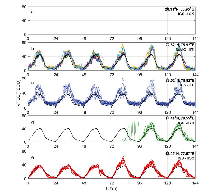
4.2.1. Storm of September 5-9, 2017
According to the National Oceanic and Atmospheric Administration (NOAA)
space weather scales (SWPC-NOAA (2017)), a G4 level (Kp =8, severe) geo-
magnetic storm was observed at 23:50 UT on September 7, 2017. There were
two more at 01:51 UT and at 13:04 UT on September 8, 2017, as a result of
a CME arrival on September 6, 2017. The CME event continued till Septem-
ber 7, 2017. Fig.15 shows VTEC (in TECU) plotted as a function of UT
(in hours) during the period of September 5-9, 2017, according to latitudes
going from north to south i.e Lucknow, Indore, Hyderabad, and Bengaluru
along with the values of the monthly mean TEC of the respective stations.
Although, the Dst dropped to a minimum value of -124 nT at 02:00 UT on
September 8, 2017, as observed in Fig. 14, the maximum TEC enhancement
(Fig.15), among these days, was observed on September 7, 2017, from all
the stations. NavIC observed a rise in TEC value in accordance with the
GPS observations. The peak TEC on September 7, 2017, from NavIC and
GPS, were 67.63 TECU and 66.78 TECU respectively, thus establishing it-
self to be reliable in monitoring geomagnetic storms. Fig.15 also indicates a
TEC enhancement of about 20-33 TECU over the quiet time monthly mean
values (plotted in black) at Lucknow, 10-20 TECU enhancement at Indore,
2-10 TECU from Hyderabad and 4-11 TECU from Bengaluru. The monthly
mean value of TEC is comparatively low for near equator locations than the
off-equatorial stations. The presence of EIA was responsible for the increased
TEC at Indore over the near equator locations. The effect of this geomag-
netic storm is also more pronounced in the EIA crest region than low latitude
13locations. One can also note the occurrence of peak TEC is slightly shifted
towards later local times as one moves from near equator to off-equatorial
sites.
4.2.2. Storm of September 25-30, 2017
A G3 level (Kp =7, strong) geomagnetic storm, according to NOAA space
weather scales, was observed on September 28, 2017. G3 level reached at
05:59 UT on September 28, 2017 and again at 08:05 UT on the same day.
Fig.16, similar to Fig.15, shows VTEC plotted as a function of UT during the
period of September 25-30, 2017, (It is to be noted that there was a data gap
in Lucknow during this period). Dst dropped to a minimum on September 28,
2017, with the value of -55 nT at 07:00 UT as observed in Fig.14 and the peak
diurnal maximum of TEC (Fig. 16), among these days, had been observed
on the same day from all the stations. On September 28, 2017, TEC values
over Indore, from NavIC and GPS were 75.73 and 77.61 TECU respectively,
further supporting the reliability of NavIC in monitoring geomagnetic storms.
It can also be seen that at Indore, the TEC enhancement is of the order of
10-35 TECU from that of quiet time monthly mean values, 16-18 TECU
over Hyderabad and 2-25 TECU over Bengaluru during this storm. From
both Fig.15 and 16, it can be observed that NavIC observables were able to
capture the geomagnetic storms similar to GPS, thereby proving itself to be
reliable in monitoring space weather events.
5. Discussions and Conclusion
NavIC is one of the recent regional navigation satellite system launched
specifically for the Indian subcontinent. Because of the availability of three
14geostationary satellites, the part of the ionosphere can be monitored continu-
ously. The additional ray path through the ionosphere due to this system can
also help to monitor space weather effects more effectively when used with
other GNSS constellations. it is observed that one of the NavIC satellite
(PRN-5) measures a part of the ionosphere where the none of GPS ray paths
are available in surrounding 1◦ x 1◦ area. This highlights another advantage
of assimilating NavIC data with GPS data for ionospheric studies over the
Indian subcontinent because of the continuous availability of NavIC signals
from all satellites throughout the day.
This paper further reveals the performance of the NavIC for studying
the space weather, evaluated at Indore using one year’s observations. To
study the performance of NavIC during severe space weather events, de-
tailed case studies of two geomagnetic storms are also presented. It has
been observed that the diurnal variation of TEC recorded from the NavIC
matches closely with that of GPS. However, the observation of a systematic
anomaly in NavIC data and may be due to the instrumental effect which
can be further investigated for a better understanding. The corrected results
indicate a consistency between GPS and NavIC which establishes NavIC as
a reliable system to probe the ionosphere. However, the analysis presented in
the paper is limited to one station of NavIC i.e., Indore, but similar compar-
ative analyses with NavIC at various stations can further be implemented
in order to validate the performance of this constellation with respect to
the Indian region. To study the performance of the NavIC system in re-
sponse to extreme space weather events, data w.r.t two geomagnetic storms
were analyzed. The enhancement of TEC was observed in both GPS and
15NavIC signals from different locations over India during the moderate storm
on September 28, 2017, and the intense storm on September 8, 2017, which
further confirms that NavIC receivers are reliable in monitoring ionospheric
response to geomagnetic storms. In both the cases, TEC estimated by NavIC
matches with that of GPS. The study confirms the reliability of the NavIC
data for ionospheric studies and will be helpful to utilize NavIC for such
studies over the equatorial ionosphere across the Indian subcontinent.
Acknowledgments
DA acknowledges the Department of Science and Technology for pro-
viding her with the INSPIRE fellowship grant to pursue her research. SC
acknowledges Space Applications Centre (SAC), ISRO for providing research
fellowship under NavIC/GAGAN utilization program: NGP-17. SAC, ISRO
is further acknowledged by the authors for providing the NavIC receiver (AC-
CORD) under NGP-17 to the Discipline of Astronomy, Astrophysics and
Space Engineering, IIT Indore. SD acknowledges the financial support re-
ceived under the INSPIRE Faculty Scheme (DST/INSPIRE/04/2014/002492)
and ISRO NGP-1. The authors would also like to acknowledge Prof. Gopi
Seemala of the Indian Institute of Geomagnetism (IIG), Navi Mumbai, India
for providing the software to analyze the IGS data.
16References
Arikan, F., Erol, C., Arikan, O., 2003. Regularized estimation of vertical
total electron content from Global Positioning System data. J.Geophys.
108, 1469. URL: https://doi.org/10.1029/2002JA009605.
Arikan, F., Nayir, H., Sezen, U., Arikan, O., 2008. Estimation of single
station interfrequency receiver bias using GPS-TEC. Radio Sci. 43. doi:10.
1029/2007RS003785.
Bandyopadhyay, T., Guha, A., DasGupta, A., Banerjee, P., Bose, A., 1997.
Degradation of navigational accuracy with Global Positioning System dur-
ing periods of scintillation at equatorial latitudes. Elect.Lett. 33, 1010–
1011. URL: https://doi:10.1049/el:19970692.
Bartels, J., 1949. The standardized index, Ks, and the planetary index, Kp,.
IATME Bull 12b, 97.
Bhardwaj, S.C., Vidyarthi, A., Jassal, B., Shukla, A.K., 2017. Study of
temporal variation of vertical TEC using NavIC data. International Con-
ference on Emerging Trends in Computing and Communication Technolo-
gies (ICETCCT) , 1–5URL: https://doi.org/10.1109/ICETCCT.2017.
8280317.
Chakraborty, S., Ray, S., Sur, D., Datta, A., Paul, A., 2020. Ef-
fects of cme and cir induced geomagnetic storms on low-latitude ion-
ization over indian longitudes in terms of neutral dynamics. Advances
in Space Research 65, 198 – 213. URL: http://www.sciencedirect.
17com/science/article/pii/S0273117719307252, doi:https://doi.org/
10.1016/j.asr.2019.09.047.
Chauhan, V., Singh, O., Singh, B., 2011. Diurnal and seasonal variation of
GPS-TEC during a low solar activity period as observed at a low latitude
station Agra. Indian Journal of Radio and Space Physics 40, 26–36.
Coco, D., Coker, C., Dahlke, S., Clynch, J., 1991. Variability of GPS satellite
differential group delay. IEEE Trans. Aerosp. Electron. Syst. 27(6), 931–
938. URL: doi:10.1109/7.104264.
Desai, M., Shweta, N., 2015. The GIVE ionospheric delay correction ap-
proach to improve positional accuracy of NavIC/IRNSS single-frequency
receiver. Current Science 114, 1665–1676. doi:10.18520/cs/v114/i08/
1665-1676.
Gonzalez, W., Joselyn, J., Kamide, Y., Kroehl, H., Rostoker, G., Tsurutani,
B., Vasyliunas, V., 1994. What is a geomagnetic storm? J. Geophys. Res
99, 5771–5792. URL: https://doi/10.1029/93JA02867.
Hunsucker, R., Hargreaves, J., 1995. The high latitude Ionosphere and its
effect on Radio propagation. Cambridge University Press.
ISRO, 2014. Indian Regional Navigation Satellite System: Signal In Space
ICD for Standard Positioning Service. ISAC, ISRO, Bangalore.
Jakowski, N., Mayer, C., Hoque, M., 2011a. A new global TEC model for esti-
mating transionospheric radio wave propagation errors. Journal of Geodesy
85, 965–974. URL: https://doi:10.1007/s00190-011-0455-1.
18Jakowski, N., Mayer, C., Hoque, M., Wilken, V., 2011b. Total Electron Con-
tent Models And Their Use In Ionosphere Monitoring. volume 46. URL:
https://doi.org/10.1029/2010RS004620.
Jee, G., Lee, H., Kim, Y.H., Chung, J., Cho, J., 2010. Assessment of GPS
global ionosphere maps (GIM) by comparison between CODE GIM and
TOPEX/Jason TEC data:Ionospheric perspective. Journal of Geophysical
Research 115. URL: https://doi.org/10.1029/2010JA015432.
Klobuchar, J.A., 1983. Ionospheric Effects on Earth-Space Propagation. Air
Force Geophys. Lab .
Klobuchar, J.A., 1996. Global Positioning System: Theory and applications,
in Ionospheric Effects in GPS. volume 1.
Komjathy, A., Langley, R., 1996. An assessment of predicted and measured
ionospheric total electron content using a regional GPS network. National
Technical Meeting of the Institute of Navigation , 615–624.
Kubo, N., Tokura, H., Pullen, S., 2018. Mixed GPS-BeiDou RTK with inter-
systems bias estimation aided by CSAC. GPS Solut. 22, 5–16. URL:
https://doi.org/10.3390/rs11121430.
Mehulkumar, D., Shweta, N., 2018. Impacts of Intense Geomagnetic Storm
on NavIC/IRNSS System. Annals of Geophysics 61,. URL: https://doi:
10.4401/ag-7856.
Misra, P., Enge, P., 2006. Global Positioning System, Signals, Measure-
ments,and Performance.
19Mitch, R.H., Psiaki, M., Tong, D., 2013. Local ionosphere model estimation
from dual-frequency global navigation satellite system observables. Radio
Sci. 48, 671–684. doi:10.1002/2013RS005153.
Mruthyunjaya, L., Ramasubramanian, R., 2017. IRNSS SIS ICD
for Standard Positioning Service. URL: https://www.isro.gov.in/
irnss-programme.
Mukesh, R., Karthikeyan, V., Soma, P., Sindhu, P., Elangovan, R., 2019.
Performance analysis of Navigation with Indian Constellation satellites.
Journal of King Saud University - Engineering Sciences URL: https://
doi.org/10.1016/j.jksues.2019.06.002.
Olatunbosun, L., Ariyibi, E., 2015. Studies of Total Electron Content vari-
ations at low-latitude stations within the Equatorial Ionization Anomaly
zone. IOSR Journal of Applied Physics (IOSR-JAP) 7, 12–24. doi:10.
9790/4861-07511224.
Olivier, J., Jean, L., Laurent, L., Lionel, R., 2015. Estimating Ionospheric
Delay using GPS/Galileo Signals in the E5 Band. InsideGNSS .
Paul, A., Chakraborty, S., DAS, A., Dasgupta, A., Mitra, S., 2005. Estima-
tion of SatelliteBased Augmentation System Grid Size at Low Latitudes
in the Indian Zone. Navigation 52, 15–22. URL: https://doi.org/10.
1002/j.2161-4296.2005.tb01727.x.
Rama Rao, P., Niranjan, K., Prasad, D.S.V.V.D., Gopi Krishna, S., Uma,
G., 2006. On the validity of the ionospheric pierce point altitude of 350km
20in the Indian equatorial and low -latitude sector. Ann. Geophys. URL:
https://doi.org/10.5194/angeo-24-2159-2006.
Ravi Kumar, M., Sridhar, M., Venkata Ratnam, D., Babu Sree Harsha, P.,
Navya Sri, S., 2019. Estimation of ionospheric gradients and vertical total
electron content using dual-frequency NAVIC measurements. Astrophys
Space Sci URL: https://doi.org/10.1007/s10509-019-3535-y.
Rethika, T., Nirmala, S., Rathnakara, S., Ganeshan, A., 2015. Ionospheric
Delay Estimation during Ionospheric Depletion Events for Single Fre-
quency Users of IRNSS. Innovative Systems Design and Engineering 6.
Roth, G., Lanyi, T., 1988. A comparison of mapped and measured total
ionospheric electron content using GPS and beacon satellite observations.
Radio Science 23.
Sampad, K., Shirish, S., Shuanggen, J., 2015. Satellite positioning
techniques-Ionospheric TEC Variations at low Latitude Indian Region.
URL: https://doi.org/10.5772/59988.
Septentrio, . URL: https://www.septentrio.com/en/products/
gnss-receivers/reference-receivers/polarx-5.
Sharma, A., Gurav, O., Anindya Bose, and Gaikwad, H., Chavan, G., Santra,
A., Kamble, S., Vhatkar, R., 2019. Potential of IRNSS/NavIC L5 signals
for ionospheric studies. Advances in Space Research URL: https://doi.
org/10.1016/j.asr.2019.01.029.
Sugiura, M., Kamei, T., 1964. Comprehensive analyses of magnetic storm
morphology. URL: http://wdc.kugi.kyoto-u.ac.jp/wdc/Sec3.html.
21SWPC-NOAA, 2017. NOAA Space Weather Scales. URL: https://www.
swpc.noaa.gov/.
Tariku, Y., 2015. Patterns of GPS-TEC variation over low-latitude regions
(African sector) during the deep solar minimum (2008 to 2009) and solar
maximum(2012 to 2013) phases . Earth, Planets and Space. 67:35. doi:10.
1186/s40623-015-0206-2.
Wu, M., Liu, W., Wang, W., Zhang, X., 2019a. Differential Inter-System
Biases Estimation and Initial Assessment of Instantaneous Tightly Com-
bined RTK with BDS-3, GPS, and Galileo. Remote Sens. 11, 1430. URL:
https://doi.org/10.3390/rs11121430.
Wu, M., Zhang, X., Liu, W., Wu, R., Zhang, R., Le, Y., Wu, Y., 2019b. Influ-
encing factors of differential inter-system bias and performance assessment
of tightly combined GPS, Galileo, and QZSS relative positioning for short
baseline. J. Navigation. 72, 965–986.
Yehuda, B., Peng, F., Melgar, D., 2016. Physical Applications of GPS
Geodesy. URL: http://sopac.ucsd.edu/dataBrowser.shtml.
22Figure 1: Latitude vs Longitude plot of Ionospheric Pierce Points (IPP) for all NavIC and
GPS satellites observed at DAASE, IIT Indore.
23Figure 2: The GPS (red) ray paths in the 1◦ x1◦ grid surrounding the IPP for each of the
NavIC satellite (NavIC-2 to 7(blue))
24Figure 3: The scatter plot between NavIC and GPS derived VTEC for a period of one year
(a) VTEC estimates without any corrections (b) VTEC estimates after making diurnal
minimum value corrections without removal of anomalous data (c) VTEC estimates after
making diurnal minimum value corrections with removal of anomalous data. Color bar
indicates the number of data points.
25Figure 4: The scatter plot between NavIC and GPS derived VTEC for the quiet days.(a)
VTEC estimates without any corrections (b) VTEC estimates after making diurnal min-
imum value corrections without removal of anomalous data (c) VTEC estimates after
making diurnal minimum value corrections with removal anomalous data. Color bar indi-
cates the number of data points.
26Figure 5: The scatter plot between NavIC and GPS derived VTEC for the disturbed
days.(a) VTEC estimates without any corrections (b) VTEC estimates after making di-
urnal minimum value corrections without removal of anomalous data (c) VTEC estimates
after making diurnal minimum value corrections with removal anomalous data. Color bar
indicates the number of data points.
27Figure 6: The anomalous data spotted in NavIC VTEC. (a) The diurnal pattern of VTEC
of NavIC (b) The zoomed-in version of (a) representing the anomalous data during quiet
ionospheric time (20-24UT)
28Figure 7: The magnitude of overestimates in NavIC derived TEC over GPS derived TEC
(a) before removal of anomalous data; (b) after removal of anomalous data for individual
NavIC satellites.
29Figure 8: Distribution (∆T ECN G (%)) of all days for each of the NavIC satellites (a) with-
out any corrections (b) after making diurnal minimum value corrections without removal
of anomalous data (c) after making diurnal minimum value corrections with anomalous
data removed.
30Figure 9: Distribution (∆T ECN G (%)) of Quiet Days for each of the NavIC satellites.(a)
without any corrections (b) after making diurnal minimum value corrections without re-
moval of anomalous data (c) after making diurnal minimum value corrections with anoma-
lous data removed.
31Figure 10: Distribution (∆T ECN G (%)) of Disturbed Days for each of the NavIC satel-
lites.(a) without any corrections (b) after making diurnal minimum value corrections with-
out removal of anomalous data (c) after making diurnal minimum value corrections with
anomalous data removed.
32Figure 11: ∆T ECN G (%) distribution over the study period combining all NavIC satel-
lites. (a) without any corrections (b) after making diurnal minimum value corrections
without removal of anomalous data (c) after making diurnal minimum value corrections
with removal of anomalous data
33Figure 12: ∆T ECN G (%) distribution during Quiet days combining all NavIC satellites
(a) without any corrections (b) after making diurnal minimum value corrections with-
out removal of anomalous data (c) after making diurnal minimum value corrections with
removal of anomalous data
34Figure 13: ∆T ECN G (%) distribution during Disturbed days combining all NavIC satel-
lites (a) without any corrections (b) after making diurnal minimum value corrections
without removal of anomalous data (c) after making diurnal minimum value corrections
with removal of anomalous data
35Figure 14: Hourly Dst values (nT) plotted as a function of days of the month of September
2017. Instances of intense storm on September 8 and moderate storm on September 28
are observed as Dst reached a minimum (marked as red ellipses) of -124 nT on September
8 and -55 nT on September 28, 2017.
36Figure 15: Variation of VTEC (in TECU) as a function of UT (in hours) during period
from September 5-9, 2017 for the stations: (a) Lucknow, (b-c) Indore, (d) Hyderabad and
(e) Bengaluru. The monthly mean TEC values for the respective stations are shown in
black.
37Figure 16: Variation of VTEC (in TECU) as a function of UT (in hours) during period
from September 25-30, 2017 for the stations:(a) Lucknow, (b-c) Indore, (d) Hyderabad
and (e) Bengaluru. The monthly mean TEC values for the respective stations are shown
in black.
38You can also read