Towards Improved Generalization in Financial Markets with Synthetic Data Generation
←
→
Page content transcription
If your browser does not render page correctly, please read the page content below
Towards Improved Generalization in Financial
                                                        Markets with Synthetic Data Generation

                                                               Brandon Da Silva                              Sylvie Shang Shi∗
                                                                    OPTrust                                 University of Toronto
arXiv:1906.03232v1 [q-fin.ST] 24 May 2019

                                                             Toronto, ON M5C 3A7                           Toronto, ON M5S 2T9
                                                            bdasilva@optrust.com                       shang.shi@mail.utoronto.ca

                                                                                              Abstract
                                                         Training deep learning models that generalize well to live deployment is a chal-
                                                         lenging problem in the financial markets. The challenge arises because of high
                                                         dimensionality, limited observations, changing data distributions, and a low signal-
                                                         to-noise ratio. High dimensionality can be dealt with using robust feature selection
                                                         or dimensionality reduction, but limited observations often result in a model that
                                                         overfits due to the large parameter space of most deep neural networks. We propose
                                                         a generative model for financial time series, which allows us to train deep learning
                                                         models on millions of simulated paths. We show that our generative model is able
                                                         to create realistic paths that embed the underlying structure of the markets in a way
                                                         stochastic processes cannot.

                                            1       Introduction
                                            In a financial markets context, "big data" often refers to the number of features one can use in their
                                            model, as opposed to the number of observations. The one exception is high frequency data, which
                                            has millions of observations per security. However, if we are designing a strategy with a longer time
                                            horizon, such as multiple days or weeks, then parameters have to be learned from a limited number
                                            of observations. As a result, many quantitative researchers reduce their feature set, at the expense of
                                            accuracy, to avoid the curse of dimensionality [26].
                                            To increase the number of observations in a data set, other domains have used data augmentation as an
                                            effective method [22]. While popular techniques for image augmentation like cropping, flipping, and
                                            rotating are not applicable for financial time series, there are a couple papers that propose solutions
                                            for time series [15, 7]. Another way to increase the number of observations in a data set is to generate
                                            synthetic data, which is the approach taken in this paper. We use a deep generative model, which
                                            typically requires a lot of training data. As such, we take inspiration from qplum’s work on recycling
                                            high frequency data [17], and use high frequency data to train the generative model. Specifically,
                                            we use AUDUSD bid prices from May 1, 2009 - December 31, 2018, which is publicly available at
                                            www.truefx.com. Since the model generates synthetic high frequency data, we use style transfer on
                                            the generated paths, as shown in Figure 1, to transfer the distributional characteristics of daily data
                                            onto our generated paths.
                                            Historically, stochastic processes have been used as the primary method to simulate asset prices
                                            because the low signal-to-noise ratio has led many to believe that markets follow a random walk.
                                            However there are important temporal dependencies embedded in asset prices which can be observed
                                            when looking at autocorrelation plots (Figure 3). Conversely, stochastic processes have a mean
                                            autocorrelation of ∼ 0 and a small standard deviation of ∼ 0.02 across runs and across lags. We
                                            chose a one-dimensional convolutional neural network (CNN) [16] as the underlying architecture for
                                                ∗
                                                    Research was done during Sylvie’s co-op term at OPTrust

                                            Preprint. Under review.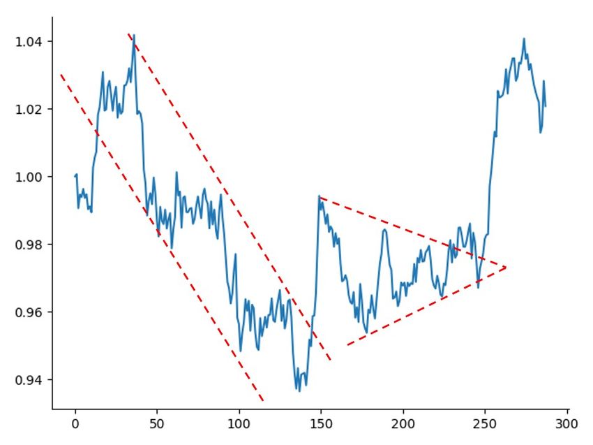
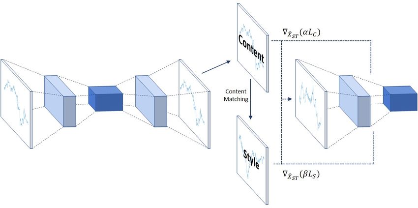
Figure 1: Although our model uses a 1D CNN, we show a 2D CNN for ease of illustration. All
paths are converted to returns and normalized before going through the CNN. Corrupted returns go
into the Denoising Autoencoder (DAE) to generate X̂. The generated paths serve as the content
in style transfer. Content-matching is then used to get the appropriate style paths. The gradient
∇X̂ST (αLC + βLS ) is used to update the style transfer paths.

our generative model because we believe the temporal dependencies in asset prices happen locally.
CNNs are great at identifying local patterns because the filters look for the same patterns everywhere
in the time series, which is not the case for popular sequence modelling architectures like LSTM and
GRU [12, 8, 5]. Additionally, technical analysts believe asset prices form a hierarchy of patterns,
which can be efficiently modelled with CNNs since they construct various levels of abstractions for an
input. The existence of market patterns can be attributed to behavioural biases and the self-reinforcing
loop that occurs because trading these patterns impacts the price of the asset being traded [21].
Comparing variance estimators at different sampling frequencies was used to test the random walk
hypothesis and show that stock prices do not follow a random walk [18]. We extend this test to
AUDUSD and find similar conclusions. Both the historical path and the generated paths from our
model reject the null hypothesis under this specification test, while three forms of stochastic processes
fail to reject the null. This indicates that our generative model captures some of the non-random local
patterns that stochastic processes are not able to capture.
We believe that considering paths which have not yet happened, but retain the underlying characteris-
tics of how asset prices move locally, will allow us to make models that generalize better. Although
we are primarily concerned with the improvement it will have on deep learning, it can also be used to
come up with more robust trading heuristics and better scenario-based risk modelling. The limiting
factor is that inputs are restricted to price action and the features that can be derived from it, such as
technical indicators.

2   Random Walk Hypothesis
The random walk hypothesis is a popular theory in the financial markets which states that financial
price series evolve with a geometric Brownian motion (GBM) [23] and are not related to historical
data, which is also known as the weak form of the efficient market hypothesis. The popular stochastic
pricing model relies entirely on this theory. More formally, a stochastic process St is said to follow a
GBM if it satisfies the following partial differential equation:

                                       dSt = µSt dt + σSt dWt
where µ is the constant drift term, σ is the volatility term and Wt is a Wiener process or Brownian
motion. By substituting Xt = log(St ) and applying Itô’s Lemma we can solve the above equation as:

                                                    2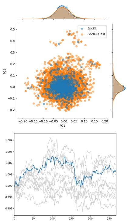
1          √
                                  Xt = X0 + (µ − σ 2 )t + σ tεt
                                                2
where εt denotes the normal disturbance of a random walk that is identically and independently
distributed. This is the strongest form of the random walk hypothesis (RW1).
In researching synthetic data generation methods, we tested the theory that time series in the financial
markets do not follow random walks and thus generating prices using a stochastic model will not
yield ideal results. We implemented the variance ratio test for the random walk hypothesis which
debuted in Lo and MacKinlay’s paper: Stock Markets Do Not Follow Random Walks: Evidence
From a Simple Specification Test [18]. This test was made robust to the second degree of random
walks, which corresponds to a GBM where the volatility of the disturbance, εt , is independent but
not identically distributed. The heteroscedasticity includes both deterministic changes in volatility
and ARCH processes in which the volatility depends on past information. This test for the random
walk hypothesis is based on the fact that for two Brownian motions Bt and Bs , the variance of the
increment, V ar(Bt − Bs ), is linear in the observation interval. In other words,

                                 V ar(Xt − Xs ) = (t − s)V ar(εt )

We can use this property to test for the null (RW1 and RW2) hypothesis by taking ratios of variances
σc2 and σa2 where:

                      σa2 = V ar(Xt − Xt−1 ) and σc2 = V ar(Xt − Xt−q )

The robustness of this test was examined by plotting the variance ratios σc2 /σa2 with time series of
different lengths. Variance ratios of time series generated by GBMs with changing volatility and
GARCH(1, 1) both converge to unity as sample size grows indefinitely. Table 1 shows that historical
data rejects the random walk hypothesis, while classic stochastic models and volatility models fail to
reject the null hypothesis. This result motivated us to continue researching for a more effective way
of synthetic data generation.

3   Generative Model

Although it has not been the focus for generative models, some work has been done on financial
time series generation. In the related work, a heuristic-based multivariate approach is used [9]. They
focus on generating hypothetical but plausible financial time series by matching some of the observed
stylized facts in the markets. While we agree with their assumption that classic models do not capture
the nuances of real price action, we prefer an unsupervised approach. By using a heuristic-based
approach, they are imposing a prior on the generation process, which ultimately limits the set of
generated paths they can produce.
We decided to use a Denoising Autoencoder (DAE) [28], which was shown to have a probabilistic
interpretation and be applied as a generative model [27, 3], after experimenting with popular genera-
tive models such as Generative Adversarial Networks (GANs) [11] and Variational Autoencoders
(VAEs) [14]. While the intuition behind GANs is quite elegant, they are difficult to train and often
experience mode collapse (which prevent us from generalizing), vanishing gradients, and/or unstable
updates [1]. Although some excellent solutions have been proposed [25, 2], there is still considerable
debate on which approach is best for GAN training [19].
Although GANs suffer from mode collapse, their generations tend to be sharp, which contrasts the
generations from VAEs, which tend to be diverse, blurry, and often unrealistic. VAEs experience
these problems because the latent space from which we sample during generation is too large. Let
x be an input and z be the transformation of x onto the latent space. By extension, qφ (z|x) is a
probabilistic encoder parameterized by φ and pθ (x|z) is a probabilistic decoder parameterized by θ.
For VAEs, we need to maximize the Evidence Lower Bound (ELBO):

                    L(θ, φ, x) = Eqφ (z|x) [log pθ (x|z)] − DKL (qφ (z|x) k pθ (z))

                                                   3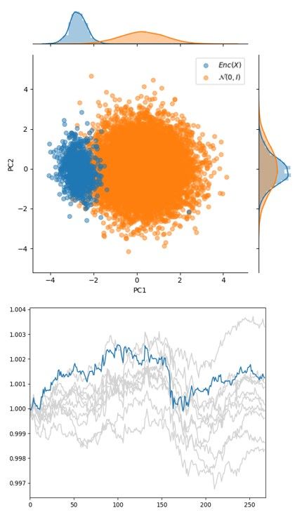
Typically, it is assumed that pθ (z) = N (0, I), which has empirically resulted in one of two con-
sequences for financial time series generation. The first is that the regularization part of ELBO,
DKL (qφ (z|x) k pθ (z)) is much easier to optimize than the log likelihood part, Eqφ (z|x) [log pθ (x|z)],
resulting in poor reconstructions. An argument could be made that this is because of the low signal-
to-noise ratio in financial markets. The second consequence is that observations cluster in the latent
space, leaving most of the probability mass in a sub region of N (0, I). We show this to be true
in Figure 2 using PCA to project the high dimensional encoding onto a 2D plane [13]. This is
problematic during generation because most of our samples z ∼ p(z) will be non-overlapping with
the actual data, z ∼ qφ (z|x). Some work has been done using GANs to find the part of the distribution
with high probability density [20, 6], however we do not see the need to decouple encoding from
generation. In fact, we want to use the encoder during generation to be confident that generated paths
are realistic.

         (a) Regular loss (VAE)     (b) Overweight reconstruction                (c) DAE
                                    loss (VAE)
Figure 2: (a) Using the regular loss function for VAEs, we see that reconstruction is poor, but qφ (z|x)
is less concentrated in p(z) than (b). Placing more weight on reconstruction during training in (b),
allowed for better reconstructions at the expense of sample quality during generation. (c) Using a
DAE shows that the actual data distribution has high probability mass under the space that we sample
from, Enc(C(x̃|x)), and it produces higher quality generations.

Let Ω define the set of paths that can be drawn from a standard normal latent space. We can also
define a subset, C ⊂ Ω, where C represents the subset of N (0, I) that can generate realistic paths. Let
B ⊂ C, in which B represents the subset of realistic path encodings that have been realized historically
for an asset. Under the assumption that realistic paths are harder to generate than unrealistic paths,
we can state that P (C) < P (C c ) and P (B)  P (B c ).
Since we are no longer using a VAE, instead of representing our encoder as a probabilistic mapping
qφ (z|x), we will use a deterministic mapping Enc(x). Under a DAE, we achieve variation in our
model by applying a corruption process on the input C(x̃|x) = x + ε, where ε ∼ N (0, σ). We then
feed the corrupted input into the encoder to generate z = Enc(C(x̃|x)). Without the corruption
process we can state that X → B, while under the corruption process X̃ → Z. Since the corruption
process involves adding Gaussian noise to the input space, we can state that |Z| > |B|. By keeping σ
to a small number in the corruption process, and because we assume |C| > |B|, we can be reasonably
certain that Z ⊂ C. Specifically, we let σ equal to half of the realized standard deviation of the input.
It might be tempting to suggest that one can just corrupt the inputs and use that as a generative
model. However, it is often the case that corrupting the inputs makes the generated paths look like
stochastic process, even with a small σ, as shown in Table 1. On the other hand, DAEs minimize

                                                    4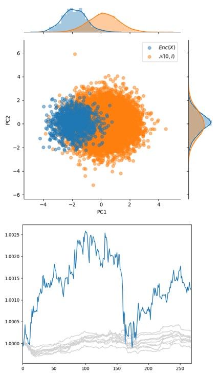
LDAE = (X̂ − X)2 , where X̂ = Dec(Enc(C(X̃|X))); it learns to reconstruct the uncorrupted
inputs from the corrupted inputs, which can only be the case if it learns to map X̃ onto the realistic
portion of the latent space, C.
Training a DAE has the added benefit of learning robust hidden representations of the underlying
paths, which we use to compute content and style loss in style transfer. We use style transfer on the
generated paths because our generative model is trained using high frequency data, but we want to
transfer the distributional characteristics (style) of daily data onto the generated high frequency paths.
Pseudo-code for the generative process is shown below:

Algorithm 1: Generate financial time series
   Input: X is the set of training paths
   Output: X̂ST is the DAE generated paths with style transfer
   if pretained model then
       θDAE ← load pretrained DAE;
   else
       θDAE ← initialize DAE parameters;
       KDAE ← epochs for DAE training;
       for i ← 0 to KDAE do
           Z ← Enc(C(X̃|X));
           X̂ ← Dec(Z);
           LDAE ← n1       (X̂ − X)2 ;
                       P
           θDAE ← θDAE − η∇θDAE (LDAE );               . Perform Adam updates for θDAE
          end
      end
      X̂ST ← initialize style transfer paths with Gaussian noise;
      KST ← epochs for style transfer training;
      for i ← 0 to KST do
          X̂ ← Dec(Enc(C(X̃|X)));
          X̂S ← style paths using content-matching;
          Fl , Pl , Sl ← feature maps in layer l for X̂ST , X̂, and X̂S ;
          LC ← 21      (Fl − Pl )2 ;
                    P

          Gl , Al ← Fl> Fl , Sl> Sl ;
                   PL
          LS ← l=0 wl 4N 21M 2        (Gl − Al )2 ;
                                    P
                             l   l

         X̂ST ← X̂ST − η∇X̂ST (αLC + βLS ) ;                    . Perform Adam updates for X̂ST
      end

4     Style Transfer

Style transfer was originally applied to images, and allows one to transfer different textures (styles)
onto an image while retaining the semantic content [10]. We extend this framework to a 1D CNN
architecture for time series. We initialize with Gaussian noise to allow the model to produce an
arbitrary number of paths, as opposed to initializing with a fixed path (usually the content) that results
in a deterministic mapping.

4.1    Application for Time Series

Style transfer has two loss functions that must simultaneously be optimized, LC and LS . Let Fl , Pl ,
and Sl be the feature maps for our style transfer, content, and style paths respectively. We use the last
layer before the encoder as our content layer, which corresponds to P   the highest level of abstractions
in our autoencoder. Thus by minimizing the content loss, LC = 21           (Fl − Pl )2 , we are retaining
the global paths from our DAE generations.

                                                     5
PL
On the other hand, for style loss, LS = l=0 wl 4N 21M 2 (Gl − Al )2 , we use the first two layers in
P
l l
the autoencoder, which correspond to lower level abstractions. Let Gl , and Al be the Gram matrices
of Fl and Sl respectively. The Gram matrix essentially measures the correlation between latent
features, where each channel represents a feature in the hidden layer. Let us consider what the
correlation between features represents in the context of a CNN. Using an RGB image as the input,
we can say that when correlation between the red and blue channel is high, both colors are present,
and thus a second-order feature, purple, is also present. Conversely, when correlation between the red
and blue channels is 0, then purple is not present in our input image. Inputs to a CNN are essentially
a combination of these second-order features since the features themselves are decompositions of the
input.
Thus, by minimizing LS , we preserve the second-order features from our daily data. Since we use
the first two layers in our DAE as style layers, we ensure that we transfer the local patterns of daily
data onto our generated paths. Note that the style layers embed more granular moves in prices than
the content layer because they deal with lower level abstractions. Thus, we maintain local patterns
and transfer the distributional characteristics of daily data onto our high frequency generated data.
4.2 Content-Matching
Before applying style transfer to the generated paths, we use content-matching as a preprocessing
step to select the style paths. Content-matching takes a generated path to be used as the content, and
iterates through all possible style paths and selects the one with the lowest content loss. Intuitively,
paths that have similar hidden representations should speed up convergence in the style transfer
process because both LC and LS are functions of the hidden representations. Empirically, we
observed this to be true.
Dynamic Time Warping (DTW) [4] and FastDTW [24] were initially explored as alternatives to
content-matching. The paths that these algorithms matched were more accurate, but they do not scale
well to thousands of paths. Let n be the sequence length of a path, M be the number of content
paths, and J be the number of possible style paths. Comparing one time series against another has a
time complexity of O(n2 ) and O(n(8r + 14)) for DTW and FastDTW respectively. Under the full
path-matching process, in which we iterate through each content path and each style path, the time
complexities go to O(JM n2 ) and O(JM n(8r + 14)) for DTW and FastDTW respectively.
For a 1D CNN, let K be the kernel size, and S be the stride size. The time complexity for a
given layer is O(K((nl − K)/(S) + 1)), where nl is the sequence length in each layer. For our
experiments we set K = S, which reduces the complexity to O(nl ) without a constant. If we take
into account the number of channels we output in each layer cl , and the number of layers L, the time
PL
complexity becomes O( l=0 nl cl ). For a large nl and a small K, nl ≈ nl−1 /S. Given we use the
first two layers for content-matching, the time complexity becomes O(n(c1 + c2 /S)). Under the full
path-matching process, the time complexity goes to O(JM n(c1 + c2 /S)).
Considering n is usually in the hundreds or thousands, DTW is eliminated as an option due to poor
scalability. Next we compare the constants for FastDTW (8r+14) and content-matching, (c1 +c2 /S).
Given our hyperparameters c1 = 8, c2 = 16, S = 3, content-matching has a lower constant than
FastDTW even with r = 1. However, if we consider the fact that a higher r is required to approach
DTW, content-matching is much faster. Ultimately we chose content-matching because it achieved
a similar speedup in style transfer convergence as DTW and FastDTW, but with a fraction of the
computational burden.
5 Experimental Results
For our experiments, we first wanted to see if our model is able to generate paths that are sufficiently
different from a random walk. To demonstrate this, we use the variance ratio test on historical paths,
corrupted historical paths, stochastic processes, and paths generated from our model. To set up the
test we show that historical paths, both high frequency and daily, reject the null hypothesis, indicating
that they do not follow a random walk. To compare, 10,000 paths were constructed with a sequence
length equal to that of daily data for each generative model. Table 1 shows that the three types of
stochastic processes fail the specification test, indeed confirming that this test is able to identify
random walks. Interestingly, when the inputs are corrupted with Gaussian noise, even with small σ,
6Table 1: Variance ratio test (q=2, 95% confidence)
Path Type p-Value Reject Null
Historical High Frequency 0.000 Reject
Historical Daily 0.006 Reject
GBM (Constant σ) 0.240 ± 0.140 Fail to Reject
GBM (Stochastic σ) 0.234 ± 0.144 Fail to Reject
GARCH(1,1) 0.232 ± 0.130 Fail to Reject
Corrupted Historical Daily 0.082 ± 0.101 Fail to Reject
DAE with Style Transfer 0.011 ± 0.029 Reject
they fail to reject the null. On the other hand, the paths that were generated with our model reject the
null, indicating that they do not follow a random walk.
The variance ratio test is robust to heteroscedastic increments observed in financial time series,
which means that by taking ratios of variances we are really testing the statistical significance of
autocorrelations in the data [18]. Thus, it should follow that autocorrelation is present in our model’s
generated paths and the realized paths, but not in stochastic processes. Across all generated paths
from stochastic processes, and across 30 lags, the autocorrelation was shown to be 0 ± 0.02. This
contrasts the autocorrelation observed in historical data (Figure 3). We show that the high frequency
generated paths from our DAE lies nicely within the autocorrelation range observed across thousands
of trading days. Similarly, after applying style transfer, our synthetic daily path lies within the same
range as our style path (content-matched realized daily path).
(a) Autocorrelation range for high frequency data and (b) Autocorrelation for style transfer path
autocorrelation for DAE generated path
Figure 3: Autocorrelation confirms generated paths are realistic
In Figure 4, we show the generation process for the paths that were used in Figure 3. Initially we
thought a simple volatility scaling of returns could be appropriate to transform the high frequency
path to a daily path. But this would leave autocorrelation and higher order moments unchanged. By
applying style transfer to the DAE generated paths, we are able to match the autocorrelation range,
skew, and kurtosis of daily data, in addition to the mean and standard deviation.
Lastly, we conducted a visual inspection of our generated paths and were impressed to see that they
embed popular technical patterns observed in asset price movements; our process generates realistic
paths that embed the structure of the markets. Technical analysts will be familiar with two very
common patterns shown in Figure 5: channels (not to be confused with CNN channels) and triangles.
We found similar patterns in hundreds of our generated paths, but struggled to find similar patterns
in paths generated with stochastic processes. Occasionally we found channels in GBM (constant σ)
generated paths, but nothing as clear as our approach. Both GBM (stochastic σ) and GARCH(1,1)
were unable to produce realistic technical patterns.
7(a) Content (b) Style (c) Style Transfer
Figure 4: We first generate a high frequency path using our DAE, which is used as the content. Then
we use content-matching to find the best style path, and ultimately use both to generate (c)
Figure 5: An example of a path generated from DAE with style transfer. There is a clear down trend
followed by a reversal, a continuation pattern, and then a breakout to the upside.
6 Conclusion
In this paper we introduced a generative model which produces realistic financial time series. The
simulated paths can be used to train deep learning models, construct robust trading heuristics, and
conduct more realistic scenario-based risk modelling. We demonstrated that our generated paths do
not follow a random walk, and display some of the popular patterns observed in the markets. Future
work will be focused on extending this framework to allow for multivariate path generation, in which
the complex relationships between time series are encapsulated in the generation process.
Acknowledgments
We thank Alex Yau and Tazeen Ajmeri for their assistance with VAE experimentation during their
time at OPTrust.
References
[1] Martin Arjovsky and Léon Bottou. Towards principled methods for training generative adver-
sarial networks. arxiv. 2017.
[2] Martin Arjovsky, Soumith Chintala, and Léon Bottou. Wasserstein generative adversarial
networks. In International Conference on Machine Learning, pages 214–223, 2017.
[3] Yoshua Bengio, Li Yao, Guillaume Alain, and Pascal Vincent. Generalized denoising auto-
encoders as generative models. In Advances in Neural Information Processing Systems, pages
899–907, 2013.
8[4] Donald J Berndt and James Clifford. Using dynamic time warping to find patterns in time series.
In KDD workshop, volume 10, pages 359–370. Seattle, WA, 1994.
[5] Junyoung Chung, Caglar Gulcehre, KyungHyun Cho, and Yoshua Bengio. Empirical evaluation
of gated recurrent neural networks on sequence modeling. arXiv preprint arXiv:1412.3555,
2014.
[6] Jesse Engel, Matthew Hoffman, and Adam Roberts. Latent constraints: Learning to generate
conditionally from unconditional generative models. arXiv preprint arXiv:1711.05772, 2017.
[7] Hassan Ismail Fawaz, Germain Forestier, Jonathan Weber, Lhassane Idoumghar, and Pierre-
Alain Muller. Data augmentation using synthetic data for time series classification with deep
residual networks. arXiv preprint arXiv:1808.02455, 2018.
[8] Thomas Fischer and Christopher Krauss. Deep learning with long short-term memory networks
for financial market predictions. European Journal of Operational Research, 270(2):654–669,
2018.
[9] Javier Franco-Pedroso, Joaquin Gonzalez-Rodriguez, Jorge Cubero, Maria Planas, Rafael Cobo,
and Fernando Pablos. Generating virtual scenarios of multivariate financial data for quantitative
trading applications. arXiv preprint arXiv:1802.01861, 2018.
[10] Leon A Gatys, Alexander S Ecker, and Matthias Bethge. Image style transfer using convolutional
neural networks. In Proceedings of the IEEE conference on computer vision and pattern
recognition, pages 2414–2423, 2016.
[11] Ian Goodfellow, Jean Pouget-Abadie, Mehdi Mirza, Bing Xu, David Warde-Farley, Sherjil
Ozair, Aaron Courville, and Yoshua Bengio. Generative adversarial nets. In Advances in neural
information processing systems, pages 2672–2680, 2014.
[12] Sepp Hochreiter and Jürgen Schmidhuber. Long short-term memory. Neural computation,
9(8):1735–1780, 1997.
[13] Ian Jolliffe. Principal component analysis. Springer, 2011.
[14] Diederik P Kingma and Max Welling. Auto-encoding variational bayes. arXiv preprint
arXiv:1312.6114, 2013.
[15] Arthur Le Guennec, Simon Malinowski, and Romain Tavenard. Data augmentation for time
series classification using convolutional neural networks. In ECML/PKDD workshop on
advanced analytics and learning on temporal data, 2016.
[16] Yann LeCun, Patrick Haffner, Léon Bottou, and Yoshua Bengio. Object recognition with
gradient-based learning. In Shape, contour and grouping in computer vision, pages 319–345.
Springer, 1999.
[17] QPLUM LLC. Use of hypothetical data in machine learning trading strategies. https://
slides.com/gchak/hypothetical-data-machine-learning-trading-strategies#
/, September 2018.
[18] Andrew W Lo and A Craig MacKinlay. Stock market prices do not follow random walks:
Evidence from a simple specification test. The review of financial studies, 1(1):41–66, 1988.
[19] Mario Lucic, Karol Kurach, Marcin Michalski, Sylvain Gelly, and Olivier Bousquet. Are gans
created equal? a large-scale study. In Advances in neural information processing systems, pages
700–709, 2018.
[20] Alireza Makhzani, Jonathon Shlens, Navdeep Jaitly, Ian Goodfellow, and Brendan Frey. Adver-
sarial autoencoders. arXiv preprint arXiv:1511.05644, 2015.
[21] John J Murphy. Technical analysis of the financial markets: A comprehensive guide to trading
methods and applications. Penguin, 1999.
[22] Luis Perez and Jason Wang. The effectiveness of data augmentation in image classification
using deep learning. arXiv preprint arXiv:1712.04621, 2017.
[23] Krishna Reddy and Vaughan Clinton. Simulating stock prices using geometric brownian motion:
Evidence from australian companies. Australasian Accounting, Business and Finance Journal,
10(3):23–47, 2016.
[24] Stan Salvador and Philip Chan. Toward accurate dynamic time warping in linear time and space.
Intelligent Data Analysis, 11(5):561–580, 2007.
9[25] Akash Srivastava, Lazar Valkov, Chris Russell, Michael U Gutmann, and Charles Sutton.
Veegan: Reducing mode collapse in gans using implicit variational learning. In Advances in
Neural Information Processing Systems, pages 3308–3318, 2017.
[26] Michel Verleysen and Damien François. The curse of dimensionality in data mining and time
series prediction. In International Work-Conference on Artificial Neural Networks, pages
758–770. Springer, 2005.
[27] Pascal Vincent. A connection between score matching and denoising autoencoders. Neural
computation, 23(7):1661–1674, 2011.
[28] Pascal Vincent, Hugo Larochelle, Yoshua Bengio, and Pierre-Antoine Manzagol. Extracting and
composing robust features with denoising autoencoders. In Proceedings of the 25th international
conference on Machine learning, pages 1096–1103. ACM, 2008.
10You can also read