HANDS-ON LAB GUIDE FOR IN PERSON ZERO-TO- SNOWFLAKE - To be used with the Snowflake free 30-day trial at
←
→
Page content transcription
If your browser does not render page correctly, please read the page content below
HANDS-ON LAB GUIDE FOR IN PERSON ZERO-TO- SNOWFLAKE To be used with the Snowflake free 30-day trial at: https://trial.snowflake.com Works for any Snowflake edition or cloud provider Approximate duration: 90 minutes. Approximately 7 credits used.
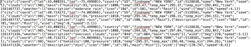
Table of Contents

Lab Overview
Module 1: Prepare Your Lab Environment
Module 2: The Snowflake User Interface & Lab “Story”
Module 3: Preparing to Load Data
Module 4: Loading Data
Module 5: Analytical Queries, Results Cache, Cloning
Module 6: Working With Semi-Structured Data, Views, JOIN
Module 7:   Using Time Travel
Module 8:   Roles Based Access Controls and Account Admin
Module 9:   Data Sharing
Summary & Next Steps

                                                            Page 1
Lab Overview
This entry-level lab introduces you to the user interface and basic capabilities of Snowflake, and is
designed specifically for use with the Snowflake, free 30-day trial at https://trial.snowflake.com. When
done with the lab you should be ready to load your own data into Snowflake and learn its more
advanced capabilities.
Target Audience
Database and Data Warehouse Administrators and Architects
What you'll learn
The exercises in this lab will walk you through the steps to:
● Create stages, databases, tables, views, and warehouses
● Load structured and semi-structured data
● Query data including joins between tables
● Clone objects
● Undo user errors
● Create roles and users, and grant them privileges
● Securely and easily share data with other accounts
Prerequisites
● Use of the Snowflake free 30-day trial environment
● Basic knowledge of SQL, and database concepts and objects
● Familiarity with CSV comma-delimited files and JSON semi-structured data
Page 2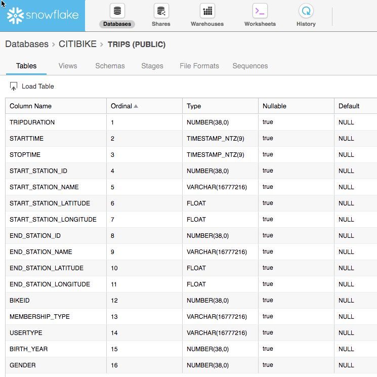
Module 1: Prepare Your Lab Environment
1.1 Steps to Prepare Your Lab Environment
1.1.1 If not yet done, register for a Snowflake free 30-day trial at https://trial.snowflake.com
● The Snowflake edition (Standard, Premier, Enterprise, e.g.), cloud provider (AWS,
Azure, e.g.), and Region (US East, EU, e.g.) do *not* matter for this lab. But we
suggest you select the region which is physically closest to you. And select the
Enterprise edition so you can leverage some advanced capabilities that are not
available in lower Editions.
● After registering, you will receive an email with an activation link and your Snowflake
account URL. Bookmark this URL for easy, future access. After activation, you will
create a user name and password. Write down these credentials.
1.1.2 Resize your browser windows so you can view this lab guide PDF and your web browser
side-by-side to more easily follow the lab instructions. If possible, even better is to use a
secondary display dedicated to the lab guide.
1.1.3 Click on
https://s3.amazonaws.com/snowflake-workshop-lab/lab_scripts_InpersonZTS.sql and
download the “lab_scripts_InpersonZTS.sql” file to your local machine. This file contains
pre-written SQL commands and we will use this file later in the lab.
Page 3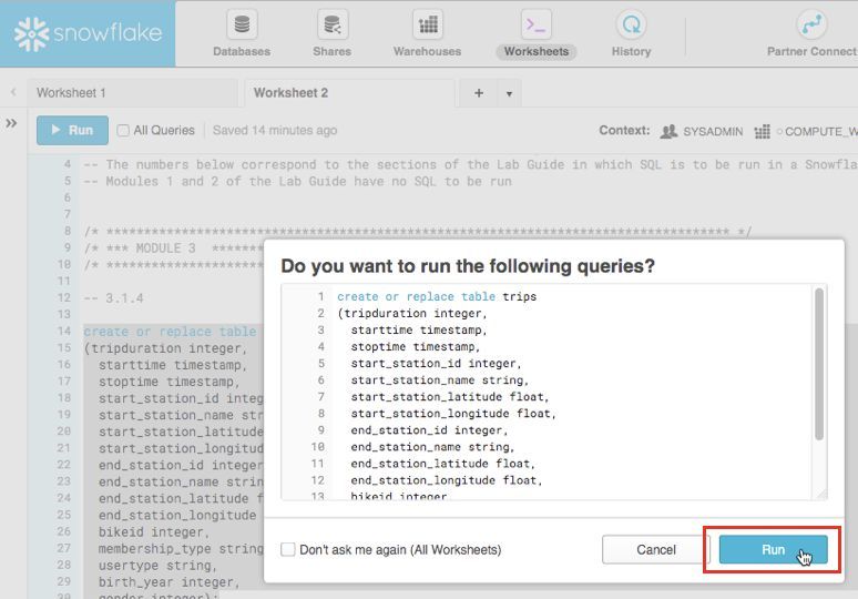
Module 2: The Snowflake User Interface & Lab “Story”
About the screen captures, sample code, and environment
Screen captures in this lab depict examples and results that may slightly
vary from what you may see when you complete the exercises.
2.1 Logging Into the Snowflake User Interface (UI)
2.1.1 Open a browser window and enter the URL of your the Snowflake 30-day trial
environment.
2.1.2 You should see the login screen below. Enter your unique credentials to log in.
2.2 Close any Welcome Boxes and Tutorials
2.2.1 You may see “welcome” and “helper” boxes in the UI when you log in for the first time.
Also a “Enjoy your free trial…” ribbon at the top of the UI. Minimize and close them by
clicking on the items in the red boxes on screenshot below.
Page 4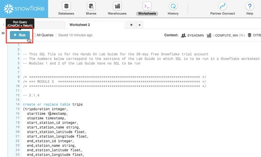
2.3 Navigating the Snowflake UI

First let’s get you acquainted with Snowflake! This section covers the basic components of the user
interface to help you orient yourself. We will move left to right in the top of the UI.

      2.3.1 The top menu allows you to switch between the different areas of Snowflake:

                                                                                        Page 5
2.3.2 The Databases tab shows information about the databases you have created or have
privileges to access. You can create, clone, drop, or transfer ownership of databases as
well as load data (limited) in the UI. Notice several databases already exist in your
environment. However, we will not be using these in this lab.
2.3.3 The Shares tab is where data sharing can be configured to easily and securely share
Snowflake table(s) among separate Snowflake accounts or external users, without
having to create a second copy of the table data. At the end of this lab is a module on
data sharing.
2.3.4 The Warehouses tab is where you set up and manage compute resources (virtual
warehouses) to load or query data in Snowflake. Note a warehouse called
“COMPUTE_WH (XL)” already exists in your environment.
Page 6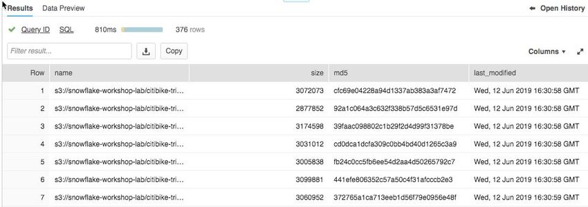
2.3.5 The Worksheets tab provides an interface for submitting SQL queries, performing DDL
and DML operations and viewing results as your queries/operations complete. The
default “Worksheet 1” appears.
In the left pane is the database objects browser which enables users to explore all
databases, schemas, tables, and views accessible by the role selected for a worksheet.
The bottom pane shows results of queries and operations.
The various windows on this page can be resized by moving the small sliders on them.
And if during the lab you need more room to work in the worksheet, collapse the
database objects browser in the left pane. Many of the screenshots in this guide will
have this database objects browser closed.
Page 7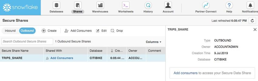
2.3.6 At the top left of the default “Worksheet 1,” just to the right of the worksheet tab, click on
the small, downward facing arrow, select “Load Script”, then browse to the
“lab_scripts.sql” file you downloaded in the prior module and select “Open”. All of the
SQL commands you need to run for the remainder of this lab will now appear on the new
worksheet. Do not run any of the SQL commands yet. We will come back to them later in
the lab and execute them one at a time.
Warning - Do Not Copy/Paste SQL From This PDF to a Worksheet
Copy-pasting the SQL code from this PDF into a Snowflake worksheet will
result in formatting errors and the SQL will not run correctly. Make sure to use
the “Load Script” method just covered.
On older or locked-down browsers, this “load script” step may not work as the
browser will prevent you from opening the .sql file. If this is the case, open the
.sql file with a text editor and then copy/paste all the text from the .sql file to the
“Worksheet 1”
Worksheets vs the UI
Much of the configurations in this lab will be executed via this pre-written SQL
in the Worksheet in order to save time. These configurations could also be
done via the UI in a less technical manner but would take more time.
2.3.7 The History tab allows you to view the details of all queries executed in the last 14 days
in the Snowflake account (click on a Query ID to drill into the query for more detail).
Page 8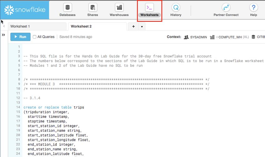
2.3.8 If you click on the top right of the UI where your user name appears, you will see that
            here you can do things like change your password, roles, or preferences. Snowflake has
            several system defined roles. You are currently in the default role of SYSADMIN and we
            will stay in this role until towards the end of this lab.

              SYSADMIN
              For most this lab you will remain in the SYSADMIN (aka System Administrator)
              role which has privileges to create warehouses and databases and other
              objects in an account.

              In a real-world environment, you would use different roles for the tasks in this
              lab, and assign the roles to your users. More on access control in Snowflake is
              in towards the end of this lab and also at
              https://docs.snowflake.net/manuals/user-guide/security-access-control.html

2.4 The Lab story
     2.4.1 This Snowflake lab will be done as part of a theoretical real-world “story” to help you
           better understand why we are performing the steps in this lab and in the order they
           appear.

                                                                                         Page 9
The “story” of this lab is based on the analytics team at Citi Bike, a real, citywide bike
share system in New York City, USA. This team wants to be able to run analytics on
data to better understand their riders and how to serve them best.
We will first load structured .csv data from rider transactions into Snowflake. This comes
from Citi Bike internal transactional systems. Then later we will load open-source,
semi-structured JSON weather data into Snowflake to see if there is any correlation
between the number of bike rides and weather.
Page 10Module 3: Preparing to Load Data
Let’s start by preparing to load the structured data on Citi Bike rider transactions into Snowflake.
This module will walk you through the steps to:
● Create a database and table
● Create an external stage
● Create a file format for the data
Getting Data into Snowflake
There are many ways to get data into Snowflake from many locations including
the COPY command, Snowpipe auto-ingestion, an external connector, or a
third-party ETL/ELT product. More information on getting data into Snowflake,
see https://docs.snowflake.net/manuals/user-guide-data-load.html
We are using the COPY command and S3 storage for this module in a manual
process so you can see and learn from the steps involved. In the real-world, a
customer would likely use an automated process or ETL product to make the
data loading process fully automated and much easier.
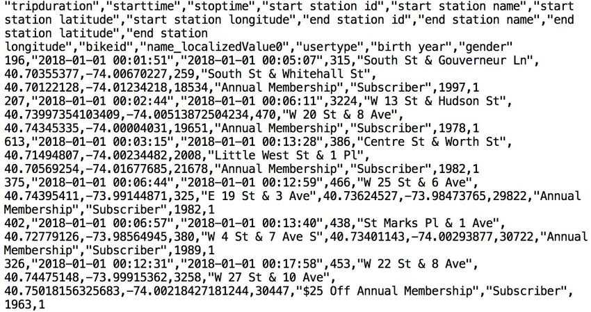
The data we will be using is bike share data provided by Citi Bike NYC. The data has been exported
and pre-staged for you in an Amazon AWS S3 bucket in the US-EAST region. The data consists of
information about trip times, locations, user type, gender, age of riders, etc. On AWS S3, the data
represents 61.5M rows, 377 objects, and 1.9GB total size compressed.
Below is a snippet from one of the Citi Bike CSV data files:
It is in comma-delimited format with double quote enclosing and a single header line. This will come
into play later in this module as we configure the Snowflake table which will store this data.
3.1 Create a Database and Table
Page 113.1.1 First, let’s create a database called CITIBIKE that will be used for loading the structured
data.
At the top of the UI select the “Databases” tab. Then click on “Create” and name the
database “CITIBIKE” and click “Finish”.
Page 123.1.2 At the top of the Snowflake UI, click the Worksheets tab. You should see the worksheet
with all the SQL we loaded in a prior step.
Page 133.1.3 First, we need to set the context appropriately within the Worksheet. In the top right, click
on the drop-down arrow next to the “Context” section to show the worksheet context
menu. Here we control what elements the user can see and run from each worksheet.
We are using the UI here to set the context. Later in the lab we will set the worksheet
context via SQL commands in the worksheet.
As needed use the downward arrows to select and show the showing:
Role: SYSADMIN
Warehouse: COMPUTE_WH (XL)
Database: CITIBIKE
Schema = PUBLIC
DDL operations are free!
Note that all the DDL operations we have done so far do NOT require compute
resources, so we can create all our objects for free.
3.1.4 Let’s now create a table called TRIPS that will be used for loading the comma-delimited
data. We will be using the Worksheets tab in the Snowflake UI to run the DDL (data
definition language) to create the table. Based on a prior step, the SQL text below should
be showing on the worksheet.
create or replace table trips
(tripduration integer,
starttime timestamp,
stoptime timestamp,
start_station_id integer,
start_station_name string,
start_station_latitude float,
Page 14start_station_longitude float,
end_station_id integer,
end_station_name string,
end_station_latitude float,
end_station_longitude float,
bikeid integer,
membership_type string,
usertype string,
birth_year integer,
gender integer);
Many Options to Run Commands.
SQL commands can be executed through the UI (limited), via the Worksheets
tab, using our SnowSQL command line tool, a SQL editor of your choice via
ODBC/JDBC, or through our Python or Spark connectors.
As mentioned earlier, in this lab we will run some operations via pre-written
SQL in the worksheet (as opposed to using the UI) to save time.
3.1.5 Run the query by placing your cursor anywhere in the command and clicking the blue
“Run” button at the top of the page or by hitting Ctrl/Cmd+Enter on your keyboard.
Warning
In this lab, never check the “All Queries” box at the top of the worksheet. We
want to run SQL queries one at a time in a specific order; not all at once.
Page 153.1.6 *If* you highlighted the entire SQL text of the command (did not just place your cursor in
the command) and ran it, a confirmation box should appear asking “Do you want to run
the following queries?”. Click the blue “Run” button in the box. In the future you can keep
clicking this “Run” button on this confirmation box or check the “Don’t ask me again (All
Worksheets)” option in this box.
Page 163.1.7 Verify that your table TRIPS has been created. At the bottom of the worksheet you
should see a “Results” section which says “Table TRIPS successfully created”
3.1.8 At the top of the page, go to the Databases tab and then click on the “CITIBIKE”
database link. You should see your newly created TRIPS table.
IMPORTANT: If you do not see the databases, expand your browser as they may be
hidden.
3.1.9 Click on the “TRIPS” hyperlink to see the table structure you just configured for it.
Page 173.2 Create an External Stage
We are working with structured, comma-delimited data that has already been staged in a public,
external S3 bucket. Before we can use this data, we first need to create a Stage that specifies the
location of our external bucket.
NOTE - For this lab we are using an AWS-East bucket. In the real-world, to prevent data
egress/transfer costs, you would want to select a staging location from the same cloud provider and
region that your Snowflake environment is in.
3.2.1 From the Databases tab, click on the “CITIBIKE” database, then click on “Stages” and
click “Create…”
Page 183.2.2 Select the option for “Existing Amazon S3 Location” and click “Next”:
3.2.3 On the “Create Stage” box that appears, enter/select the following settings, then click
“Finish”.
Name citibike_trips
Schema Name PUBLIC
URL s3://snowflake-workshop-lab/citibike-trips
NOTE - The S3 bucket for this lab is public so you can leave the key fields empty. In the “real world”
this bucket would likely require key information.
Page 193.2.4 Now let’s take a look at the contents of the citibike_trips stage. At the top of the page,
click on the Worksheet tab. Then execute the following statement:
list @citibike_trips;
You should see the output in the Results window in the bottom pane:
Page 203.3 Create a File Format
Before we can load the data into Snowflake, we have to create a File Format that matches the data
structure.
3.3.1 From the Databases tab, click on the CITIBIKE database hyperlink. Then click on “File
Formats”. Then click “Create”.
3.3.2 On the resulting page, we then create a file format. In the box that appears, leave all the
default settings as-is but make the changes below:
Name: CSV
Field optionally enclosed by: Double Quote
Null string:
[ ] Error on Column Count Mismatch:
IMPORTANT: If you do not see the “Error on Column Count Mismatch” box, scroll down in the
dialogue box
When you are done, the box should look like:
Page 21Then click on the “Finish” button to create the file format.
Page 22Module 4: Loading Data
For this module, we will use a data warehouse and the COPY command to initiate bulk loading of the
structured data into the Snowflake table we just created.
4.1 Resize and Use a Warehouse for Data Loading
For loading data, compute power is needed. Snowflake’s compute nodes are called Warehouses and
they can be dynamically sized up or out according to workload, whether the workload be loading data,
running a query, or performing a DML operation. And each workload can have its own data
warehouse so there is no resource contention.
4.1.1 Navigate to the Warehouses tab. Note the “Create…” option at the top is where you can
quickly create a new warehouse. However, we want to use the existing warehouse
“COMPUTE_WH” which comes with the 30-day trial environment.
Click on the row of this “COMPUTE_WH” warehouse (not the blue hyperlink that says
“COMPUTE_WH”) so the entire row is highlighted. Then click on the “Configure...” text
above it to see the configuration detail of the “COMPUTE_WH”. We will use this
warehouse to load in the data from AWS S3.
Page 234.1.2 Let’s walk through the settings of this warehouse as there is a lot of functionality here,
much of which is unique to Snowflake versus other data warehouses.
NOTE - If you do not have a Snowflake Edition of Enterprise or greater, you will *NOT*
see the “Maximum Clusters” or “Scaling Policy” configurations from the screenshot
below. Multi-clustering is not utilized in this lab, but we will still discuss it as it is a key
capability of Snowflake.
● The “Size” drop-down is where the size of the warehouse is selected. For larger data loading
operations or more compute-intensive queries, a larger warehouse will be needed. The t-shirt
sizes translate to underlying compute nodes, either AWS EC2 or Azure Virtual Machines. The
larger the t-shirt size, the more compute resources from the cloud provider are allocated to that
warehouse. As an example, the 4-XL option allocates 128 nodes. Also, this sizing can be
changed up or down on the fly with a simple click.
● If you have Snowflake Edition or greater you will see the Maximum Clusters section. This is
where you can set up a single warehouse to be multi-cluster up to 10 clusters. As an example,
if the 4-XL warehouse we just mentioned was assigned a maximum cluster size of 10, it could
scale up to be 1280 (128 * 10) AWS EC2 or Azure VM machines modes powering that
warehouse...and it can do this in seconds! Multi-cluster is ideal for concurrency scenarios,
such as many business analysts simultaneously running different queries using the same
warehouse. In this scenario, the various queries can be allocated across the multiple clusters
to ensure they run fast.
Page 24● The final sections allow you to automatically suspend the warehouse so it suspends (stops)
itself when not in use and no credits are consumed. There is also an option to automatically
resume (start) a suspended warehouse so when a new workload is assigned to it, it will
automatically start back up. This functionality enables Snowflake’s fair “pay as you use”
compute pricing model which enables customers to minimize their data warehouse costs.
Snowflake Compute vs Other Warehouses
Many of the warehouse/compute capabilities we just covered, like being able to
create, scale up and out, and auto-suspend/resume warehouses are things that
are simple in Snowflake and can be done in seconds. Yet for on-premise data
warehouses these capabilities are very difficult (or impossible) to do as they
require significant physical hardware, over-provisioning of hardware for
workload spikes, significant configuration work, and more challenges. Even
other cloud data warehouses cannot scale up and out like Snowflake without
significantly more configuration work and time.
Warning - Watch Your Spend!
During or after this lab you should *NOT* do the following without good reason
or you may burn through your $400 of free credits more quickly than desired:
● Disable auto-suspend. If auto-suspend is disabled, your warehouses will
continue to run and consume credits even when not being utilized.
● Use a warehouse size that is excessive given the workload. The larger
the warehouse, the more credits are consumed.
4.1.3 We are going to use this data warehouse to load the structured data into Snowflake.
However, we are first going to decrease the size of the warehouse to reduce the
compute power it contains. Then in later steps we will note the time this load takes, then
Page 25re-do the same load operation with a larger warehouse, and observe how much faster
the load is with a larger warehouse.
Change the Size of this data warehouse from X-Large to Small. Then click the “Finish”
button.
4.2 Load the Data
Now we can run a COPY command to load the data into the TRIPS table we created earlier.
4.2.1 Via the top of the UI, navigate back to the Worksheets tab and click on it. Make sure the
context is correct by setting these in the top right of the worksheet:
Role: SYSADMIN
Warehouse: COMPUTE_WH (S)
Database: CITIBIKE
Schema = PUBLIC
Page 264.2.2 Execute the following statements in the worksheet to load the staged data into the table.
This may take up to 30 seconds.
copy into trips from @citibike_trips
file_format=CSV;
In the Results window, you should see the status of the load:
Page 274.2.3 Once the load is done, at the bottom right of the worksheet click on the small arrow next
to the “Open History” text to show the history of Snowflake operations performed in that
specific worksheet.
4.2.4 In the History window see the “copy into trips from @citibike_trips file_format=CSV;”
SQL query you just ran and note the duration, bytes scanned and rows. Use the slider
on the left side of the pane to expand it if needed to see all the detail in it.
4.2.5 Go back to the worksheet to clear the table of all data and metadata, by using the
TRUNCATE TABLE command.
truncate table trips;
Page 284.2.6 At the top of the UI go to the Warehouses tab, then click on “Configure..” Resize the
warehouse to size Large and click “Finish”. This warehouse is four times larger than the
Small size.
4.2.7 Go back to the Worksheets tab at the top of the UI and click on it. Execute the following
statements in the worksheet to load the same data again.
copy into trips from @citibike_trips
file_format=CSV;
4.2.8 Once the load is done, at the bottom of the worksheet in the History window compare the
times between the two loads. The one with the Large warehouse was significantly faster.
4.3 Create a New Warehouse for Data Analytics
Going back to the lab story, let’s assume the Citi Bike team wants to ensure no resource contention
between their data loading/ETL workloads and the analytical end users using BI tools to query
Snowflake. As mentioned earlier, Snowflake can easily do this by assigning different,
appropriately-sized warehouses to different workloads. Since Citi Bike already has a warehouse for
data loading, let’s create a new warehouse for the end users running analytics. We will then use this
warehouse to perform analytics in the next module.
Page 294.3.1 At the top of the UI click on the Warehouses tab then “Create…”. Name it
“ANALYTICS_WH” with size “Large”. If you have Snowflake edition Enterprise or
greater, you will see a setting for “Maximum Clusters”. Set this to “1”.
Leave the other settings in their default settings. It should look like:
Then click on the “Finish” button to create the warehouse.
Page 30Module 5: Analytical Queries, Results Cache, Cloning
In the previous exercises, we loaded data into two tables using Snowflake’s bulk loader (COPY
command) and the warehouse COMPUTE_WH. Now we are going to pretend we are analytics users
at Citi Bike who need to query data in those tables using the worksheet and the second warehouse
ANALYTICS_WH.
“Real World” Roles and Querying
In the “real world” the analytics users would likely have a different role then
SYSADMIN; to keep the lab simple we are going to stay with the SYSADMIN
role for this module.
Also, in the “real-world” querying would typically be done with a business
intelligence product like Tableau, Looker, PowerBI, etc. Or for more advanced
analytics, data science products like Spark or R can query Snowflake. Basically
any technology that leverages JDBC/ODBC can run analytics on the data in
Snowflake. But to keep this lab simple, all queries are being done via the
Snowflake worksheet.
5.1 Execute SELECT Statements and Result Cache
5.1.1 Go the Worksheets tab. Within the worksheet, make sure you set your context
appropriately:
Role: SYSADMIN
Warehouse: ANALYTICS_WH (L)
Database: CITIBIKE
Schema = PUBLIC
5.1.2 Run the query below to see a sample of the trips data
select * from trips limit 20;
Page 315.1.3 First let’s look at some basic hourly statistics on Citi Bike usage. Run the query below in
the worksheet. It will show for each hour the number of trips, average trip duration, and
average trip distance.
select date_trunc('hour', starttime) as "date",
count(*) as "num trips",
avg(tripduration)/60 as "avg duration (mins)",
avg(haversine(start_station_latitude, start_station_longitude, end_station_latitude,
end_station_longitude)) as "avg distance (km)"
from trips
group by 1 order by 1;
5.1.4 Snowflake has a result cache that holds the results of every query executed in the past
24 hours. These are available across warehouses, so query results returned to one user
are available to any other user on the system who executes the same query, provided
Page 32the underlying data has not changed. Not only do these repeated queries return
extremely fast, but they also use no compute credits.
Let’s see the result cache in action by running the exact same query again.
select date_trunc('hour', starttime) as "date",
count(*) as "num trips",
avg(tripduration)/60 as "avg duration (mins)",
avg(haversine(start_station_latitude, start_station_longitude, end_station_latitude,
end_station_longitude)) as "avg distance (km)"
from trips
group by 1 order by 1;
In the History window note that the query runs significantly faster now because the
results have been cached.
5.1.5 Next, let's run this query to see which days of the week are the busiest:
select
dayname(starttime) as "day of week",
count(*) as "num trips"
from trips
group by 1 order by 2 desc;
Page 335.2 Clone a Table
Snowflake allows you to create clones, also known as “zero-copy clones” of tables, schemas, and
databases in seconds. A snapshot of data present in the source object is taken when the clone is
created, and is made available to the cloned object. The cloned object is writable, and is independent
of the clone source. That is, changes made to either the source object or the clone object are not part
of the other.
A popular use case for zero-copy cloning is to clone a production environment for use by
Development & Testing to do testing and experimentation on without (1) adversely impacting the
production environment and (2) eliminating the need to set up and manage two separate
environments for production and Development & Testing.
Zero-Copy Cloning FTW!
A massive benefit is that the underlying data is not copied; just the
metadata/pointers to the underlying data change. Hence “zero-copy” and
storage requirements are not doubled when data is cloned. Most data
warehouses cannot do this; for Snowflake it is easy!
5.2.1 Run the following command in the worksheet to create a development (dev) table
create table trips_dev clone trips
Page 345.2.2 If closed, expand the database objects browser on the left of the worksheet. Click the
small Refresh button in the left-hand panel and expand the object tree under the Citibike
database. Check that you can see a new table under the CITIBIKE database named
TRIPS_DEV. The development team now can do whatever they want with this table,
including even deleting it, without having any impact on the TRIPS table or any other
object.
Page 35Module 6: Working With Semi-Structured Data, Views, JOIN
NOTE - The first steps here are similar to prior Modules 3 (Preparing to Load Data) and 4 (Loading
Data) but we will do most of it via SQL in the worksheet, as opposed to via the UI, to save time.
Going back to the lab “story”, the Citi Bike analytics team wants to see how weather impacts ride
counts. To do this, in this module we will:
● Load weather data in JSON format held in a public S3 bucket
● Create a View and query the semi-structured data using SQL dot notation
● Run a query that joins the JSON data to the TRIPS data from a prior module of this guide
● See how weather impacts trip counts
The JSON data consists of weather information provided by OpenWeatherMap detailing the historical
conditions of New York City from 2016-07-05 to 2019-06-25. It is also staged on AWS S3 where the
data represents 57.9k rows, 61 objects, and 2.5MB total size compressed.
The raw JSON in GZ files and in a text editor looks like:
SEMI-STRUCTURED DATA
Snowflake can easily load and query semi-structured data, such as JSON,
Parquet, or Avro, without transformation. This is important because an
increasing amount of business-relevant data being generated today is
semi-structured, and many traditional data warehouses cannot easily load and
query this sort of data. With Snowflake it is easy!
6.1 Create a Database and Table
6.1.1 First, via the Worksheet, let’s create a database called WEATHER that will be used for
storing the unstructured data.
create database weather;
Page 366.1.2 Set the context appropriately within the Worksheet.
use role sysadmin;
use warehouse compute_wh;
use database weather;
use schema public;
6.1.3 Via the worksheet, let’s now create a table called JSON_WEATHER_DATA that will be
used for loading the JSON data. In the worksheet, run the SQL text below. Snowflake
has a special column type called VARIANT which will allow us to store the entire JSON
object and eventually query it directly.
create table json_weather_data (v variant);
Semi-Structured Data Magic
Snowflake’s VARIANT data type allows Snowflake to ingest semi-structured
data without having to pre-define the schema.
6.1.4 Verify that your table JSON_WEATHER_DATA has been created. At the bottom of the
worksheet you should see a “Results” section which says “Table
JSON_WEATHER_DATA successfully created”
Page 376.1.5 At the top of the page, go to the Databases tab and then click on the “WEATHER”
database link. You should see your newly created JSON_WEATHER_DATA table.
6.2 Create an External Stage
6.2.1 Via the Worksheet create a stage from where the unstructured data is stored on AWS
S3.
create stage nyc_weather
url = 's3://snowflake-workshop-lab/weather-nyc';
6.2.2 Now let’s take a look at the contents of the nyc_weather stage. At the top of the page,
click on the Worksheets tab. In the worksheet, then execute the following statement with
a LIST command to see the list of files:
list @nyc_weather;
You should see the output in the Results window in the bottom pane showing many gz
files from S3:
Page 386.3 Loading and Verifying the Unstructured Data
For this section, we will use a warehouse to load the data from the S3 bucket into the Snowflake table
we just created.
6.3.1 Via the worksheet, run a COPY command to load the data into the
JSON_WEATHER_DATA table we created earlier.
Note how in the SQL here we can specify a FILE FORMAT object inline. In the prior
module where we loaded structured data, we had to define a file format in detail. But
because the JSON data here is well-formatted, we use default settings and simply
specify the JSON type.
copy into json_weather_data
from @nyc_weather
file_format = (type=json);
6.3.2 Take a look at the data that has been loaded.
select * from json_weather_data limit 10;
6.3.3 Click on one of the values. Notice how the data is stored in raw JSON format. Click
“Done” when finished.
Page 396.4 Create a View and Query Semi-Structured Data
Let’s look at how Snowflake allows us to create a view and also query the JSON data directly using
SQL.
Views & Materialized Views
A View allows the result of a query to be accessed as if it were a table. Views
can help you: present data to end users in a cleaner manner (like in this lab we
will present “ugly” JSON in a columnar format), limit what end users can view in
a source table for privacy/security reasons, or write more modular SQL.
There are also Materialized Views in which SQL results are stored, almost as
though the results were a table. This allows faster access, but requires storage
space. Materialized Views require Snowflake Enterprise Edition or higher.
6.4.1 From the Worksheet tab, go into the worksheet and run the following command. It will
create a view of the unstructured JSON weather data in a columnar view so it is easier
for analysts to understand and query. FYI - the city ID for New York City is 5128638.
create view json_weather_data_view as
select
v:time::timestamp as observation_time,
v:city.id::int as city_id,
v:city.name::string as city_name,
v:city.country::string as country,
v:city.coord.lat::float as city_lat,
v:city.coord.lon::float as city_lon,
v:clouds.all::int as clouds,
(v:main.temp::float)-273.15 as temp_avg,
(v:main.temp_min::float)-273.15 as temp_min,
Page 40(v:main.temp_max::float)-273.15 as temp_max,
v:weather[0].main::string as weather,
v:weather[0].description::string as weather_desc,
v:weather[0].icon::string as weather_icon,
v:wind.deg::float as wind_dir,
v:wind.speed::float as wind_speed
from json_weather_data
where city_id = 5128638;
6.4.2 The prior step showed how you can use SQL dot notation (v.city.coord.lat) to pull out
values at lower levels in the JSON hierarchy. This allows us to treat each field as if it
were a column in a relational table.
6.4.3 Verify the view at the top left of the UI where the new view should appear just under the
table json_weather_data. You may need to expand and and/or refresh the database
objects browser in order to see it.
6.4.4 Via the worksheet, verify the view with the following query. Notice the results look just
like a regular structured data source (NOTE - your result set may have different
observation_time values)
select * from json_weather_data_view
where date_trunc('month',observation_time) = '2018-01-01'
limit 20;
Page 416.5 Use a Join Operation to Correlate Against Data Sets
We will now join the JSON weather data to our CITIBIKE.PUBLIC.TRIPS data to determine the
answer to our original question of how weather impacts the number of rides.
6.5.1 Run the command below to join WEATHER to TRIPS and count the number of trips
associated with certain weather conditions .
Note - Since we are still in a worksheet use the WEATHER database as default, we will
fully qualify our reference to the TRIPS table by providing its database and schema
name.
select weather as conditions
,count(*) as num_trips
from citibike.public.trips
left outer join json_weather_data_view
on date_trunc('hour', observation_time) = date_trunc('hour', starttime)
where conditions is not null
group by 1 order by 2 desc;
Page 426.5.2 The Citi Bike initial goal was to see if there was any correlation between the number of
bike rides and weather by analyzing both ridership and weather data. Per the table
above we have a clear answer. As one would imagine, the number of trips is significantly
higher when the weather is good!
For the rest of this lab, we will look at other capabilities of Snowflake.
Page 43Module 7: Using Time Travel
Snowflake’s Time Travel capability enables accessing historical data at any point within a
pre-configurable period of time. The default period of time is 24 hours and with Snowflake Enterprise
Edition it can be up to 90 days. Most data warehouses cannot offer this functionality; with Snowflake it
is easy!
Some useful applications of this include:
● Restoring data-related objects (tables, schemas, and databases) that may have been
accidentally or intentionally deleted
● Duplicating and backing up data from key points in the past
● Analysing data usage/manipulation over specified periods of time
7.1 Drop and Undrop a Table
First let’s see how we can restore data objects that have been accidentally or intentionally deleted.
7.1.1 From the worksheet, run the following command which will drop (remove) the
json_weather_data table:
drop table json_weather_data;
7.1.2 Now run a SELECT statement on the json_weather_data table. In the “Results” pane
you should see an error because the underlying table has been dropped.
select * from json_weather_data limit 10;
7.1.3 Now restore the table:
undrop table json_weather_data;
7.1.4 The json_weather_data table should be restored.
Page 447.2 Roll Back a Table
Now let’s look rolling back a table to a previous state to fix an unintentional DML error that replaces
all the station names in the Citibike database TRIPS table with the word “oops.”
7.2.1 First make sure the worksheet is in the proper context:
use role sysadmin;
use warehouse compute_wh;
use database citibike;
use schema public;
7.2.2 Then run the following command that replaces all the station names in the table with the
word “oops”.
update trips set start_station_name = 'oops';
7.2.3 Now run a query that returns the top 20 stations by # of rides - notice how we’ve
screwed up the station names so we only get one row:
select
start_station_name as "station",
count(*) as "rides"
from trips
group by 1
order by 2 desc
limit 20;
Page 457.2.4 Normally, we would need to scramble and hope we have a backup lying around. But in
Snowflake, we can simply run commands to find the query ID of the last UPDATE
command & store it in a variable called $QUERY_ID…
set query_id =
(select query_id from
table(information_schema.query_history_by_session (result_limit=>5))
where query_text like 'update%' order by start_time limit 1);
7.2.5 Then re-create the table as of before the update:
create or replace table trips as
(select * from trips before (statement => $query_id));
7.2.6 Run the SELECT statement again to check that the station names have been restored:
select
start_station_name as "station",
count(*) as "rides"
from trips
group by 1
order by 2 desc
limit 20;
Page 46Module 8: Roles Based Access Controls and Account Admin
In this module we will show some aspects of Snowflake roles based access control (RBAC), including
creating a new role and granting it specific permissions. We will also cover the ACCOUNTADMIN
(aka Account Administrator) role.
To continue with the Citi Bike story, let’s assume a junior DBA has joined Citi Bike and we want to
create a new role for them with less privileges than the system-defined, default role of SYSADMIN.
Let’s now do that.
Roles-Based Access Control (RBAC)
Snowflake offers very powerful and granular RBAC which can control what
objects and capabilities a role or user can access, and what level of access
they have. For more detail, see the documentation at
https://docs.snowflake.net/manuals/user-guide/security-access-control.html
8.1 Create New Role and Add User to it
8.1.1 In the worksheet let’s switch to the ACCOUNTADMIN role to create a new role. This role
encapsulates the SYSADMIN and SECURITYADMIN system-defined roles. It is the
top-level role in the system and should be granted only to a limited/controlled number of
users in your account. In the worksheet, run:
use role accountadmin;
When done, notice at the top right of the worksheet, the worksheet context has changed
so now the role is ACCOUNTADMIN
8.1.2 In order for any role to function, we need at least one user assigned to it. So let’s create
a new role called “junior_dba” and assign your user name to it. This is the user name
you created when you first opened your 30-day free trial Snowflake account. This name
also appears at the top right of the UI. In the screenshot below it is “USER123”. Of
course yours will be different. Make a note of your user name.
Page 478.1.3 Let’s now create the role and add a user to it with your unique user name:
create role junior_dba;
grant role junior_dba to user YOUR_USER_NAME_GOES HERE;
NOTE - if you tried to perform this operation while in a role like SYSADMIN, it would fail due to
insufficient privileges as the SYSADMIN role by default cannot create new roles or users.
8.1.4 Change your worksheet context to the new junior_dba role
use role junior_dba;
At the top right of the worksheet, note that the context has changed to reflect the junior_dba role
8.1.5 On the left side of the UI in the database object browser pane, notice that both the
Citibike and Weather databases do not appear. This is because the junior_dba role does
not have access to view them.
Page 488.1.6 Let’s switch back to the ACCOUNTADMIN role and grant the junior_dba the ability to
view and use the CITIBIKE and WEATHER databases
use role accountadmin;
grant usage on database citibike to role junior_dba;
grant usage on database weather to role junior_dba;
8.1.7 Switch to the junior_dba role and at the left in the database object browser, note the
Citibike and Weather databases now appear. Click the refresh icon if they do not appear.
use role junior_dba;
8.2 Account Administrator View
Let’s change our security role for the session to ACCOUNTADMIN to see other parts of the UI only
this role can see.
Roles in User Preference vs Worksheet
We just changed the security role for the session in the user preference menu
at the top right of the UI. This changes what we can see in the UI. This is
different then the worksheet context menu where we assign a role that is
applied to the commands run on that specific worksheet. Also, session security
role can simultaneously be different from the role used in a worksheet.
Page 498.2.1 In the top right corner of the UI, click on your user name to show the User Preferences
menu. Then go to Switch Role, then select the ACCOUNTADMIN role.
8.2.2 Notice at the very top of the UI you will now see a sixth tab called “Account” that you can
only view in the ACCOUNTADMIN role.
Click on this Account tab. Then towards the top of this page click on “Usage” which by
default already appearsI. Here you see detail on credits, storage, and daily usage.
8.2.3 To the right of “Usage” is “Billing” where you can add a credit card if you want to go
beyond your free $400 worth of credits for this free trial. Further to the right is information
on Users, Roles, and Resource Monitors. The latter set limits on your account's credit
consumption so you can appropriately monitor and manage credit consumption.
NOTE - Stay in the ACCOUNTADMIN role for the next module.
Page 50Module 9: Data Sharing
Snowflake enables account-to-account sharing of data through shares, which are created by data
providers and “imported” by data consumers, either through their own Snowflake account or a
provisioned Snowflake Reader account. The consumer could be an external entity/partner, or a
different internal business unit which is required to have its own, unique Snowflake account.
With Data Sharing –
● There is only one copy of data, which lives in the data provider’s account
● Shared data is always live, real-time and immediately available to consumers
● Providers can establish revocable, fine-grained access grants to shares
● Data sharing is simple and secure, especially compared to the “old” way of sharing data which
was often manual and involved transferring large .csv across the Internet in a manner that
might be insecure
Note - Data Sharing currently only supported between accounts in the same Snowflake
Provider and Region
One example of data sharing is that Snowflake uses secure data sharing to share account usage
data and sample data sets with all Snowflake accounts. In this capacity, Snowflake acts as the
provider of the data and all other accounts act as the consumers. In your Snowflake environment you
can easily see this and we walk through this in the next section.
Page 519.1 See Existing Shares
9.1.1 Click on the blue Snowflake logo at the very top left of the UI. On the left side of the UI
in the database object browser, notice the database “SNOWFLAKE_SAMPLE_DATA”,
The small arrow on the database icon indicates this is a share.
9.1.2 At the top right of the UI verify you are in the ACCOUNTADMIN role. Then at the top of
the UI click on the Shares tab. Notice on this page you are looking at your Inbound
Secure Shares and there are two shares shared by Snowflake with your account. One
contains your account usage and the other has sample data you can use. This is data
sharing in action - your Snowflake account is a consumer of data shared/provided by
Snowflake!
Page 529.2 Create an Outbound Share
9.2.1 Let’s go back to the Citi Bike story and assume we are the Account Administrator for
Snowflake at Citi Bike. We have a trusted partner who wants to do perform data science
on the data in our TRIPS database on a near real-time basis to further analyze it. This
partner also has their own Snowflake account in our region. So let’s use Snowflake Data
Sharing to share this data with them so they can analyze it.
At the top of the UI click on the Shares tab. Then, further down on the page click on the
“Outbound” button.
9.2.2 Click on the “Create” button and in the fields that appear, fill them out as shown below.
● For “Secure Share Name” enter “TRIPS_SHARE”
● For “Database” you will use the drop-down to select “CITIBIKE”
● For “Tables & Views” you will use the database object browser to browse to CITIBIKE >
PUBLIC > TRIPS.
● Click on the blue “Apply” button
Page 539.2.3 Click on the blue “Create” button at the bottom of the box.
Note the window indicates the Secure share was created successfully.
Page 54In the real-world, the Citi Bike Account Administrator would click on the “Next: Add
Consumers” blue button to add information on their partner’s Snowflake account name
and type. But since in the lab we are just using our own account, we will stop here.
9.2.4 Click on the “Done” button at the bottom of the box.
Note this page now shows the “TRIPS_SHARE” secure share. It only took seconds to
give other accounts access to data in Snowflake in a secure manner with no copies of
the data having to be made!
Page 55Lastly, note that Snowflake provides several ways to securely share data without
compromising confidentiality. You can share not only tables and views, but also Secure
Views, Secure UDFs (User Defined Functions), and Secure Joins. For more details on
how to use these methods for sharing data while preventing access to sensitive
information, see the Snowflake documentation.
Congratulations, you are now done with this lab! Let’s wrap things up in the next, and
final, section.
Page 56Summary & Next Steps
This tutorial was designed as a hands-on introduction to Snowflake to simultaneously teach you how
to use it, while showcasing some of its key capabilities and differentiators. We covered how to
navigate the UI, create databases and warehouses, load & query structured and semi-structured
data, perform zero-copy cloning, undo user errors, RBAC, and data sharing.
We encourage you to continue with your free trial by loading in your own sample or production data
and by using some of the more advanced capabilities of Snowflake not covered in this lab. There are
several ways Snowflake can help you with this:
● At the very top of the UI click on the “Partner Connect” icon to get access to trial/free ETL and
BI tools to help you get more data into Snowflake and then analyze it
● Read the “Definitive Guide to Maximizing Your Free Trial” document at:
https://www.snowflake.com/test-driving-snowflake-the-definitive-guide-to-maximizing-your-free-
trial/
● Attend a Snowflake virtual or in-person event to learn more about our capabilities and how
customers use us https://www.snowflake.com/about/events/
● Contact Sales to learn more https://www.snowflake.com/free-trial-contact-sales/
Resetting Your Snowflake Environment
Lastly, if you would like to reset your environment by deleting all the objects created as part of this
lab, run the SQL below in a worksheet.
Run this SQL to set the worksheet context:
use role accountadmin;
use warehouse compute_wh;
use database weather;
use schema public;
Then run this SQL to drop all the objects we created in the lab:
drop share if exists trips_share;
drop database if exists citibike;
drop database if exists weather;
drop warehouse if exists analytics_wh;
drop role if exists junior_dba;
Page 57You can also read