Metrological evaluation of efficiency and consumption of domestic gas cooking appliances - International Journal of ...
←
→
Page content transcription
If your browser does not render page correctly, please read the page content below
Int. J. Metrol. Qual. Eng. 12, 16 (2021)                                                                        International Journal of
© R. Medeiros Moreira and E.C. de Oliveira, Published by EDP Sciences, 2021                           Metrology and Quality Engineering
https://doi.org/10.1051/ijmqe/2021015
                                                                                                                 Available online at:
                                                                                                               www.metrology-journal.org

    RESEARCH ARTICLE

Metrological evaluation of efficiency and consumption
of domestic gas cooking appliances
Rosana Medeiros Moreira1,2 and Elcio Cruz de Oliveira2,3,*
1
    National Institute of Technology, Venezuela Avenue, 82, Centro, 20081-312 - Rio de Janeiro, Brazil
2
    Posgraduate Metrology Programme, Rio de Janeiro Catholic University, Marquês de São Vicente Street, 225, Gávea,
    Rio de Janeiro  Brazil
3
    Technology Management, PETROBRAS TRANSPORTE S.A., Rio de Janeiro  Brazil

            Received: 28 January 2021 / Accepted: 3 June 2021

            Abstract. This study evaluates the results of efficiency and consumption tests on gas household appliances and
            their influence on the classification of the Brazilian Labeling Program. Historically, based on results in
            interlaboratory comparisons, there is a doubt concerning if the algorithms correct properly the differences
            among different altitudes. Data from efficiency and consumption tests were collected in two cities with different
            altitudes, and the proposed calculation methodology is compared with the traditional one. The results show that
            the arithmetic average, used in the calculation of the efficiency of the burners on the stove table, justifies being
            replaced by the weighted average, after evaluating the behaviour of the data and treating outliers. The
            uncertainty of the efficiency and consumption tests was not enough to change the classification range of the
            product’s energy efficiency label. It is concluded that statistically a difference is observed between the results at
            sea level and at altitude above sea level; since the tests were applied by the same operator using the same
            apparatus, the only parameter that leaves a doubt is the algorithms for the correction of the altitude. Shortly,
            this study will be part of a revised Brazilian standard.
            Keywords: Altitude / Brazilian standard / consumption / measurement uncertainty /
            thermal efficiency / stoves

1 Introduction                                                              manufacturers must comply with increasingly rigid
                                                                            efficiency indexes, regulated by Brazilian Metrology
Brazil, following the example of developed countries, has                   Institute [3] and measured by means of tests following
been making a great effort in the implementation of                         European technical standard [4].
product certification and labeling programs, mainly for                          Products linked to the use of fuels such as alcohol
those that have popular use and that bring some risk to the                 containers for domestic use, canisters of liquefied petro-
user. Currently, there are numerous products with                           leum gas (LPG) and cylinders of natural gas (CNG), due to
compulsory certification, forcing manufacturers and                          their high degree of risk of accidents, were prioritized in the
importers of stoves to adopt measures to comply with                        certification programs. Meanwhile, domestic gas cooking
the maximum levels of energy consumption and minimum                        appliances are labeled under the Brazilian Labeling
energy efficiency (or energy performance). This ensures                      Program, PBE.
greater quality assurance for countless products, greater                       PBE is an energy conservation program that, by means
safety, excludes manufacturers that do not meet minimum                     of informative labels, aims to guide the consumer regarding
quality and safety conditions, promotes greater competi-                    the energy efficiency of some products sold in the country.
tiveness, and still opens space for exports, in addition to                 Its objective is to stimulate the rationalization of energy
creating barriers for imported products without quality [1].                consumption by using products that are more efficient.
    Gas stoves must comply with the Brazilian Policy for                    Labeling allows the consumer to evaluate the various
Conservation and Rational Use of Energy [2], in which                       products in terms of their energy efficiency and select the
                                                                            ones that bring the greatest savings during use.
                                                                                The labeling program for domestic gas cooking
* Corresponding author: elciooliveira@puc-rio.br                            appliances, using more efficient stoves and ovens, aims

This is an Open Access article distributed under the terms of the Creative Commons Attribution License (https://creativecommons.org/licenses/by/4.0),
             which permits unrestricted use, distribution, and reproduction in any medium, provided the original work is properly cited.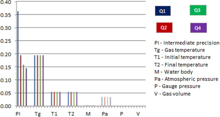
2                     R. Medeiros Moreira and E.C. de Oliveira: Int. J. Metrol. Qual. Eng. 12, 16 (2021)

to encourage the rationalization of gas consumption in         relation to sea level, the air has less oxygen per unit volume;
general, especially LPG. Therefore, this program is in line    therefore, the gas-burning rate must be adjusted to
with the goals of the Brazilian Energy Plan (PNE2030) [5]      maintain adequate combustion of the fuel. This can be
and the Brazilian Energy Efficiency Plan (PNEf) [6].            done by decreasing the size of the fuel injector orifice in the
    The labeling of domestic gas cooking appliances was        burner to reduce the equivalence rate. Wieser et al. [10]
instituted by an Brazilian Interministerial Decree [7],        carried out a series of comparative experiments at different
signed by the Brazilian Ministry of Industry, Foreign          altitudes; that is, from 400 m to 3000 m and observed that
Trade and Services (MDIC), Brazilian Ministry of Mines         with the increase in altitude, the burning rate is reduced
and Energy (MME) and Brazilian Ministry of Science and         because of the decrease in atmospheric pressure.
Technology.                                                        The heating capacity of the stove is also affected by the
    The labeling of gas stoves and ovens is mandatory and      change in the air density, because due to the lower density,
the Brazilian Energy Conservation Label  ENCE                 the air has less heat transport capacity, because the hot air
provides information on the Power, efficiency, consump-         has a lower density than the cold air, that by convection
tion and internal volume of the oven. The standardization      phenomenon, the hot air goes up and the cooler air goes
of this information allows a better evaluation and power of    down. Amell [11] studied the effect of energy in domestic
choice for the consumer, providing a natural process of        atmospheric burners for LPG or natural gas (NG) in
incentive to manufacturers for technological improvement       Colombian locations such as Santa de Antioquia (555 m),
resulting in increased efficiency, operational safety and       Medellín (1550 m) and Alto Bogotá (2600 m). The result
reduced cost of sale. Labeling is an important mechanism       of this study stated that the performance of an
for industrial competitiveness and can also contribute to      atmospheric burner decreases 1.5% by 304 m of altitude
the success of other objectives aimed at economic and social   increase. An experimental analysis of thermal efficiency,
development.                                                   power and emissions of liquefied petroleum gas in stoves at
    To receive ENCE, gas stoves and ovens need to be           altitudes between 2200 and 4200 meters in Peru are
approved in all the defined and standardized criteria           presented [12]. The studies concluded that power,
pertinent to the Conformity Assessment Regulation             efficiency and combustion vary according to the altitude
RAC.                                                           above sea level.
    When the PBE of gas stoves and ovens started in Brazil         More recently, Zhou et al. [13] investigated the
20 years ago, there were only two laboratories accredited by   influence of altitude on power, thermal efficiency and
ISO / IEC 17025. Since, the results of the tests carried out   emissions in domestic atmospheric burners for NG in the
by the laboratories did not converge statistically, the        Chinese locations of Lhasa (3658 m) and Chongqing
Technical Group for the study of the RAC met and decided       (4000 m). The study concluded that a change in fuel gas
that the problem was due to the corrections of the altitude    supply pressure could compensate for the energy loss that is
parameter and that the mathematical models applied to          produced with increasing altitude, that thermal perfor-
the European standard [4] did not make the correct             mance increases as altitude increases, and that emissions
correction of atmospheric pressure. This working group         increase by decreasing oxygen in atmospheric air at a
decided to replace the existing algorithm in the standard,     higher altitude when compared to sea level.
with the formula for the correction of the nominal Power           Brazilian Metrology Institute, in the use of its
contained in the European standard [8] without, however,       attributions as regulator of the gas appliances sector,
an in-depth technical-scientific study. The standard has        established in 2008, the specific regulation for the use of the
not been revised and the doubt persists nowadays, whether      national energy conservation label  ENCE. This regula-
this correction is really adequate, because even after         tion defines the technical and operational requirements
appropriate corrections, the results of interlaboratory        imposed on the Brazilian system for the assessment of
plans do not converge if carried out at sea level or at        conformity for gas stoves and ovens produced and or
other altitudes.                                               marketed in Brazilian territory. The specific regulation was
    Therefore, aim of this study is to metrologically          approved and instituted with the publication of joint
evaluate the results of the performance and consumption        ordinance 73, of April 5, 2002 [14]. In January 2008,
tests on domestic gas cooking appliances and their             Inmetro published Ordinance 018 [15] and revised specific
influence on the PBE classification, based on the statistical    Regulation 008, the same that was in force until 2012. In
treatments of the data obtained in these tests.                August 1, 2012, Inmetro Ordinance No. 400 [3] was
                                                               published. The new regulation for conformity assessment
                                                               (RAC), contained in this ordinance, emphasizes the types
2 Methodology                                                  of devices covered by the scope, the indices, the classifica-
                                                               tion ranges and in the annex, the control metrology
The stove is a relatively simple device for combustion. Its    required to ensure the quality of the required products and
burner is a type of pre-mix and multi-hole door, and           services. This document also sets the energy rating ranges
operates at low pressure (2.75 kPa), Surange et al. [9].       for table and oven burners, Table 1.
   A gas burner is a device for generating a flame to heat          On October 10, 2013, Inmetro published Ordinance
products using fuels such as natural gas or liquefied           No. 496 [16] in which it establishes the deadlines for
petroleum gas. Some burners have an air inlet to mix the       extinction of old products in commerce on August 1, 2014
combustible gas with the air to make a complete                and determines that the deviations between the amount
combustion, Surange et al. [9]. At higher altitudes in         declared in the spreadsheet of the technical specification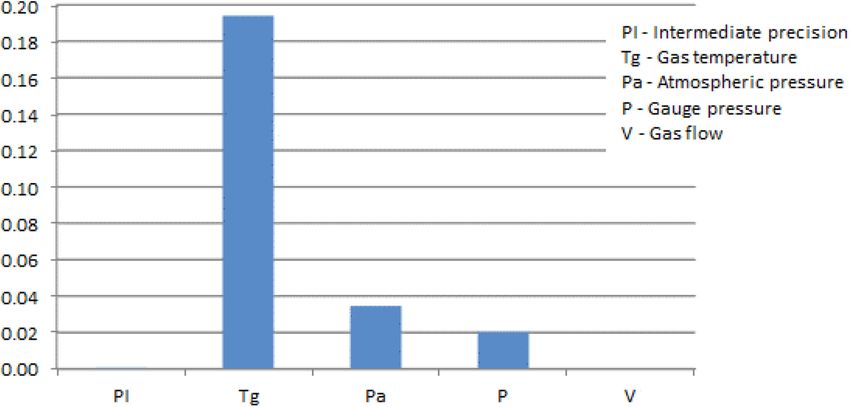
R. Medeiros Moreira and E.C. de Oliveira: Int. J. Metrol. Qual. Eng. 12, 16 (2021)                                     3

Table 1. Energy rating for table and oven burners.

Average burner efficiency of the table, h (%)                Consumption index of the oven CI (%)                                Classification PBE
h ≥ 63                                                      CI  49                                                             A
61  h   <   63                                             49 < CI      53                                                    B
59  h   <   61                                             53 < CI      57                                                    C
57  h   <   59                                             57 < CI      60                                                    D
52  h   <   57                                             60 < CI      63                                                    E

Table 2. Allowable nominal deviations in the initial test.          where:
                                                                        M1 is the body of water used (inside the test vessel),
Burner table efficiency (h)                                  ±3%     in kg;
                                                                        m is the mass of the test vessel and its lid, in kg;
Oven consumption index (CI)                                 ±5%
                                                                        Crec is the specific heat of the test vessel (aluminium),
Oven volume (V)                                             ±2%     in MJ/kg °C.
                                                                        Vn is the volume of gas used, in m3, corrected to
                                                                    the reference conditions (101.33 kPa, 15 °C) of Hs by
of efficiency and of the appliance’s energy consumption              equation (3).
must comply with the limits specified in Table 2.
    The determination, in accordance with the regulations                                           P a þ P  W 288:15
                                                                                      Vn ¼ V
described above, of table performance (h) and oven                                                      101:33 273:15 þ T g
consumption (CI), follows the test procedure specified by
                                                                                                                 Pa þ P  W
[4] and [8]; measuring quantities for use as variables in the                                  ¼ 2:84368V                     ½m3             ð3Þ
calculation equations of h and CI, described as follow.                                                          273:15 þ T g
    Regarding the spread of measurement uncertainty, the
combined uncertainty will be calculated according to [17],          where:
for both h and CI and considering the input quantities as               V is the volume read under the test conditions (Pa, P, Tg),
not correlated with each other.                                     in m3;
                                                                        Pa is the local atmospheric pressure, in kPa;
                                                                        P is the gas supply pressure in the meter, in kPa;
2.1 Efficiency measurement of domestic gas cooking                       Tg is the gas temperature at the measurement point,
appliances                                                          in °C;
                                                                        W is the saturation pressure of water vapor at
The calculation of the efficiency ( ), in %, equation (1), is
                                                                    temperature Tg, in kPa, equation (4).
expressed according to the test conditions.

                   Heat absorbed         MCðT 2  T 1 Þ
                                                                                                                    5262
                                                                                                          21:094273:15þT
         h¼                        ¼ 100                                                              e                     g
                  Heat transferred         V nHs                               W ¼ W Tg ¼
                                                                                                   10
                         M ðT 2  T 1 Þ
              ¼ 0:4186                  ½%                   ð1Þ                                      5262
                            V nHs                                                ¼ 0:1 exp 21:094                 ½kPa                       ð4Þ
                                                                                                    273:15 þ T g
where:                                                                 By processing equations (1)–(4), a more detailed and
    Heat absorbed refers to the effective heating of the test       explicit form of the efficiency equation is obtained in the
vessel;                                                             dependent variables, equations (4) and (5) assists in the
    Heat transferred refers to the combustion energy of the         propagation of uncertainties of the input quantity Vn.
volume of gas used;
    C is the specific heat of the water, 4.186  103 MJ/kg °C;
    T1 is the initial temperature of the test vessel (20 ± 1) °C;              h ¼ hðM;T 2 ;T 1 ;Hs;V ;P a ;P ;T g Þ
    T2 is the maximum water temperature after the flame is                                                                           1 1
extinguished (90 ± 1) °C;                                                       ¼ 0:4186ðM 1 þ 0:213mÞðT 2  T 1 Þ                         ½% ð5Þ
                                                                                                                                    Hs V n
    Hs is the gross calorific value of the gas used, if it is the
reference gas, butane, it will be constant and equal to
126.21 MJ/m3, without associated uncertainty, i.e.,                                                                    Pa þ P  W
negligible uncertainty [8].                                               V n ¼ V nðV ;P a ;P ;T g Þ ¼ 2:84368V                     ½m3       ð6Þ
                                                                                                                       273:15 þ T g
    M is the equivalent mass of the test vessel, equation (2);

                          C rec                                        The efficiency sensitivity coefficients in relation to M,
             M ¼ M1 þ           m ¼ M 1 þ 0:213m ½kg         ð2Þ   T1, T2, and Hs depend only on equation (3) and are
                           C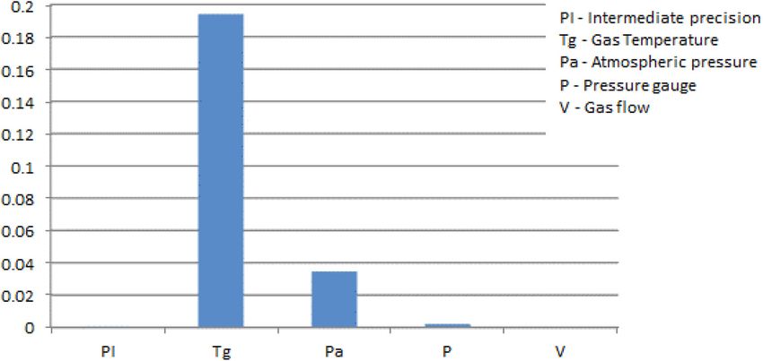
4                               R. Medeiros Moreira and E.C. de Oliveira: Int. J. Metrol. Qual. Eng. 12, 16 (2021)

described according to equations (7)–(10).                                15 °C and under a pressure of 101.33 kPa, as described by
                                                                          [8]. The purpose of equation (16) is to convert the
               F h;M ¼
                           ∂h
                              ¼
                                   h
                                                     ½%=kg         ð7Þ   volumetric flow measured in the test conditions (V_ ) for
                          ∂M M 1 þ 0:213m                                 a flow value in the reference conditions (V_ c)
                                                                                    sffiffiffiffiffiffiffiffiffiffiffiffiffiffiffiffiffiffiffiffiffiffiffiffiffiffiffiffiffiffiffiffiffiffiffiffiffiffiffiffiffiffiffiffiffiffiffiffiffiffiffiffiffiffiffiffiffiffiffiffiffiffiffiffiffiffiffiffiffiffiffiffiffiffiffiffiffiffiffiffiffiffiffiffiffiffi
                                 ∂h      h                                           101:33 þ P P a þ P 288:15 dhðP a ;P ;T g Þ
                  F h;T 2 ¼         ¼              ½%=°C           ð8Þ   V_ c ¼ V_                                                                                         ½m3 =h
                                ∂T 2 T 2  T 1                                            101:33 101:33 273:15 þ T g                                          dr
                                                                                                                                                                           ð16Þ
                         ∂h     h
            F h;T 1   ¼     ¼          ¼ F h;T 2         ½%=°C    ð9Þ
                        ∂T 1 T 2  T 1                                       If a wet meter is used or if the gas used is saturated, the
                                                                          value d (relative density of dry gas in relation to dry air)
                                                                          shall be replaced by the value of the relative density of the
                                ∂h   h
                F h;Hs ¼           ¼        ½% kg °C=MJ           ð10Þ   wet gas dh given by equation (equation 17):
                               ∂Hs Hs
   As Vn depends on V, Pa, P, Tg, and W, where W                                           P a þ P  W ðT g Þ d þ 0:622W ðT g Þ
depends on Tg, there will be no sensitivity coefficient in Vn,                       dh ¼
                                                                                                         Pa þ P
but rather in V, Pa, P e Tg according to equations (11) and
(14).                                                                                          0:622  d
                                                                                       ¼dþ               W ðT g Þ                  ð17Þ
                                                                                                Pa þ P
                                  ∂h h
                        F h;V ¼      ¼          ½%=m3             ð11Þ   where:
                                  ∂V   V
                                                                              V_ is the gas flow measured in the test conditions, in
                                                                          m /h;(Pa, P, Tg), in m3/h;
                                                                            3
                           ∂h       h
              F h;P a ¼       ¼                     ½%=kPa        ð12Þ       Pa is the local atmospheric pressure, in kPa;
                          ∂P a P a þ P  W                                    P is the gas supply pressure in the meter, in kPa;
                                                                              Tg is the temperature of the gas at the measurement
                                                                          point, in °C;
                 ∂h      h
     F h;P ¼        ¼           ¼ F h;P a            ½%=kPa       ð13Þ       d is the relative density of the dry (or wet) test gas
                 ∂P P a þ P  W                                           relative to dry air;
                                                                              dr is the relative density of the dry reference gas relative
             ∂h       h            5262W                                  to dry air;
F h;T g ¼       ¼                           2 F h;P a ½%=°C               W is the saturation pressure of the water vapor at the
            ∂T g 273:15 þ T g    273:15 þ T g                             temperature Tg (Eq. 4), in kPa.
                                                                   ð14Þ      Equation (15) for the burner consumption can then be
                                                                          rewritten to cover all the quantities measured in the test
                                                                          (Eq. 18).
2.2 Measurement of consumption of domestic gas
                                                                          Pc ¼ P  _
cooking appliances                                                               c V ;H s ;P ;P a ;T g
                                                                                               sffiffiffiffiffiffiffiffiffiffiffiffiffiffiffiffiffiffiffiffiffiffiffiffiffiffiffiffiffiffiffiffiffiffiffiffiffiffiffiffiffiffiffiffiffiffiffiffiffiffiffiffiffiffiffiffiffiffiffiffiffiffiffiffiffiffiffiffiffiffi
The burner consumption test, Pc, referred to as “consump-                                    _      101:33 þ P P a þ P 288:15 dh
                                                                             ¼ 0:278 HsV                                                                               ½kW
tion” by [4], goes by means of an initial temperature                                                   101:33 101:33 273:15 þ T g dr
stabilization step (210 ± 1 °C) above room temperature,
being then calculated by equation (15):                                                                                                                                    ð18Þ

                  P ¼ 0:278 _
                           c V_ H ½KW  c   s         ð15Þ                      dh ¼ dhðP a ;P ;T g Þ , see equation (17)
where:                                                                          W ¼ W ðT g Þ [kPa], see equation (4)
    Pc is consumption, in kW;
    0.278 is the conversion factor of consumption, in                        The efficiency sensitivity coefficients in relation to V_
kW/(MJ/h);                                                                and Hs depend only on equation (18) and are described
    Hs is the higher calorific value of the gas used (if it is the         according to equations (19) and (20).
reference gas, butane, it will be constant and equal to
                                                                                                             ∂P c P c                  h        i
126.21 MJ/m3, without associated uncertainty, i.e.,
                                                                                                F        _ ¼     ¼                      kW h=m3                            ð19Þ
negligible uncertainty [8].                                                                         P c ;V   ∂V_   V_
    V_ c is the volumetric flow, of the gas under the reference
conditions (101.33 kPa and 15 °C), obtained from equation                                                           ∂P c   Pc
(16), in m3/h.                                                                                     F P c ;Hs ¼           ¼                  ½g °C=s                       ð20Þ
                                                                                                                    ∂Hs Hs
    The volumetric flow corresponds to the measurement of
a reference gas flow (99.99% pure butane m/m) under                            As dh depends on Pa, P, Tg, and W, where W depends on
reference conditions, that is, assuming the gas is dry, at                Tg, there will be no sensitivity coefficient of Pc in dh, but in
R. Medeiros Moreira and E.C. de Oliveira: Int. J. Metrol. Qual. Eng. 12, 16 (2021) 5
Table 3. Summary of the steps of statistical processes.
Aim/Statistical test Normal distribution Non-normal distribution
Assessment of normality Shapiro-Wilk
Outliers Grubbs’ test Interquartile range (IQR)
1 1
Position measurement pi ¼ pi ¼ 2
s 2i MAD=0:6745 i
MAD ¼ Median ½jxi Median ðxi Þj
Xm Xm
x :p
i¼1 i i
M i :pi
x¼ X m Md ¼ X i¼1
m
p
i¼1 i
p
i¼1 i
Uncertainty Assessment Law of propagation of uncertainties It is not relevant in this study
Pa, P, and Tg according to equations (21)–(23). 2.4 Uncertainty of table efficiency tests and oven
consumption
∂P c 1 P c d The combined standard uncertainties of efficiency and
F P c ;P a ¼ ¼ ½W=Pa ð21Þ
∂P a 2 P a þ P dh consumption are calculated by equation (25) and the
expanded uncertainty will be equal to the combined
standard uncertainty, multiplied by the coverage factor
∂P c P a þ P dh (k = 2; for infinite degrees of freedom) to obtain an interval
F P c ;P ¼ ¼ F P c ;P a þ1 ½W=Pa with a confidence level of (p = 95.45%), equation (26).
∂P 101:33 þ P d
ð22Þ
XN
∂f 2 2
u2c ðyÞ ¼ u ðxi Þ ð25Þ
∂P c 1 Pc ∂xi
F P c ;T g ¼ ¼ i¼1
∂T g 2 273:15 þ T g
5262 dh d U ðyÞ ¼ k uc ðyÞ ð26Þ
1 ½W=Pa ð23Þ
273:15 þ T g dh
2.5 Statistical testing steps
2.3 Calculation of the oven consumption index
This study proposes a methodology for the statistical
The calculation of the furnace consumption index (CI), for treatment of data based on the assessment of data
stoves and liquefied petroleum gas (LPG) ovens, equation normality, the treatment of outliers and the calculation
(24). of the average efficiency based on the position measure-
ment weighted by the measure of dispersion of each burner
[18], Table 3.
C Where: pi is the weight and must be related to the
ICGLP ¼ 100 ð24Þ
ð0:93 þ 0:035 V F Þ 0:0726 variability of the data, and quantified by means of standard
deviations, s i; x is average; Md is median; i is the index that
refers to each of the experimental values available, xi is the
where: measure of efficiency, ISO GUIDE 35 [19].
VF is the volume in dm3;
0.0726 is the local atmospheric pressure, in kPa;
C is the consumption of maintenance of the oven, where 3 Summary of test method and experimental
the amount of gas per unit of time supplied for combustion data
in the oven burner to maintain, in the geometric center of
the empty oven, the temperature rise of 210 °C above the A table burner is covered with a 220 mm diameter
ambient temperature. This quantity is expressed in kg/h, container, containing 3.7 kg of water, which must be
for LPG [3]; operated for 10 minutes at nominal power. Such a 220 mm
(0.93 + 0.035 VF) is consumption, expressed in kilo- container is removed and immediately replaced by the
watts, and calculated on Hs. specific container to be used in the performance test.6 R. Medeiros Moreira and E.C. de Oliveira: Int. J. Metrol. Qual. Eng. 12, 16 (2021)
Table 4. Mass of water as a function of the burner power.
Burner power about the Hs in (kW) Internal diameter of container in (mm) Body of water M1 in (kg)
Between 1.16 and 1.64 220 3.7
Between 1.64 and 1.98 240 4.8
Between 1.99 and 2.36 2601) 6.1
Between 2.37 and 4.20 2601),2) 6.1
1)
If the container with a diameter of 260 mm cannot be used, the test must be conducted under the normal conditions of use of the
appliance, using the 240 mm container with corresponding M1 water mass, and the burner power must be adjusted to 1.98 kW (on Hs).
2)
With a burner power setting to 2.36 kW (over Hs).
Fig. 1. Assembly configuration of the test bench.
For the performance test, a wet gas flow meter is used. With the empty oven, the flow of the register is
It is a semi-submerged rotor meter, which controls the adjusted, so that in the steady state the temperature rise,
aspiration and escape of the gas whose flow you want to measured in the geometric center of the empty oven. This
measure is done through the liquid, which has a sealing measurements is made by a thermocouple, is at 210 °C ±
function. For flow measurement, one lobe has its outlet end 1 °C above the ambient temperature or, if the maximum
submerged and that of the emerged inlet, aspirating gas, possible temperature rise is less than 210 °C, corresponding
and the other has the submerged inlet and the emerged to the maximum position of the thermostat or register,
outlet, expelling gas. Therefore, this type of meter moistens with the same tolerance. The temperature adjustment
the air, changing its relative density and leading to the need must be done by changing the position of the register and/
to use the term dh/dr in equation (16). or varying the nominal pressure of the reference gas
The initial water temperature must be 20 °C ± 1 °C and by ±5%.
the water temperature at the time of extinguishing the In the measurement of the performance and consump-
flame in the burner must be 90 °C ± 1 °C. tion tests of domestic stoves, nine measurements were
M is the equivalent mass of the test vessel, according to made on each burner (Qi) of the stove table and nine
the indications in Table 4. measurements on the oven burner, by the same operator
For the consumption test the oven burner is fed with using the same apparatus, at sea level (Laboratory A) and
reference gas (butane 99.9% m/m), regulated with a above the level of the sea, 935 m (Laboratory B). The
pressure of 2.75 kPa and the ambient temperature must measurement configuration is described in Figure 1 and
remain throughout the test at 20 ° C ± 5 ° C. these results are available in Table 5.R. Medeiros Moreira and E.C. de Oliveira: Int. J. Metrol. Qual. Eng. 12, 16 (2021) 7
Table 5. Experimental data.
Laboratory A Laboratory B
Q1 (%) Q2 (%) Q3 (%) Q4 (%) Oven (kg/h) Q1 (%) Q2 (%) Q3 (%) Q4 (%) Oven (kg/h)
63.9 67.7 66.7 62.0 0.117 62.3 64.5 64.2 60.3 0.106
62.6 67.0 66.3 61.4 0.122 60.6 64.6 64.2 60.0 0.100
64.1 67.4 66.2 62.3 0.122 63.4 67.1 66.2 60.3 0.115
62.5 67.9 67.1 61.2 0.120 62.5 67.6 66.3 60.0 0.110
65.5 68.4 67.2 62.6 0.119 63.3 64.9 65.6 60.4 0.112
63.9 68.8 65.7 62.1 0.122 62.9 65.8 66.4 60.3 0.114
62.0 68.6 66.8 61.9 0.116 63.0 67.9 66.9 60.7 0.115
64.4 68.3 66.8 61.9 0.118 63.1 67.2 66.2 60.8 0.112
63.6 68.0 66.4 62.2 0.119 63.9 67.7 66.7 60.9 0.112
4 Results and discussion After applying the Grubbs and IQR tests, respectively,
for the efficiency and consumption tests, it was observed
Data from Laboratories A and B are handled by two that no data sets have outliers.
different approaches. The first approach is the traditional The performance test data set showed a normal
one that is based on [4]; that is, arithmetic mean of the data distribution; therefore, the estimate of the quantity, from
without analysis and treatment of the data. The second the average, is weighted inversely proportional to their
approach, here proposed, is based on the current statistical respective variances and finally, the average efficiency of
tests, Table 3. the National Energy Conservation Label is calculated by
The measurement uncertainty evaluation regarding the the weighted average.
intermediate precision of the efficiency and consumption For this data set, one can infer from Table 6 that the
methods was calculated from the grouped standard means of the four burners compared cannot be considered
deviation of the nine tests performed on each burner, equal. That is, there is a significant difference between the
repeated under the same conditions, so we are faced with a data sets (F > F-critical), so that we cannot consider them
Type A uncertainty, whose standard uncertainty experi- as being samples from the same population. Anova shows
that the use of the arithmetic mean of the four burners is
mental average is given by uðxi Þ ¼ spðxffiffiniffiÞ, where s (xi) is the not statistically compatible. Thus, the average weighted by
experimental standard deviation for n observations. the variance is justified.
Whereas the uncertainties contributions are type B Considering the specification range, according to
assessments are provided by the calibration certificates: Inmetro Ordinance 400 of August 1, 2012 [3], the efficiency
– Efficiency: water and gas temperature (thermometer), according to the national energy conservation label, affixed
atmospheric pressure (barometer), gas pressure (ma- to the equipment, is 63% ± 3%, that is, (61% to 65%). The
nometer) and gas volume (volumetric meter); result of Laboratory A is framed by the traditional
– Consumption: gas temperature (thermometer), atmo- approach, 65% (arithmetic average) and the proposed
spheric pressure (barometer), gas pressure (manometer) approach 65% (weighted average).
and gas volume (volumetric meter).
The calculation of the efficiency ( ) is given by 4.2 Evaluation of the results of Laboratory B
equation (1) and input quantities for the combined
standard uncertainty are given by equations (5) and (6). Based on Shapiro Wilk’s test, with the exception of burner
The sensitivity coefficients (ci) are presented from 3, all efficiency results have a normal distribution. In turn,
equations (8)–(14). the consumption results have a behaviour that departs
The calculation of the consumption (Pc) is given by from the normality:
equation (15) and input quantities for the combined After the treatment of outliers with the application of
standard uncertainty are given by equation (18). The the Grubbs test in the performance test in Q1, Q2 and Q4,
sensitivity coefficients (ci) are presented from equations and IQR in the performance test in Q3, and also in the
(19)–(22). consumption test, it was observed with a new application of
the Shapiro-Wilk test that all experimental data started to
4.1 Evaluation of the results of Laboratory A have a normal distribution.
The data set of the performance tests showed a normal
Based on Shapiro Wilk’s test, all efficiency and consump- distribution, therefore, the estimate of the quantity, from
tion results have a normal distribution: the average, is weighted inversely proportional to their8 R. Medeiros Moreira and E.C. de Oliveira: Int. J. Metrol. Qual. Eng. 12, 16 (2021)
Table 6. Anova of the results of the burner efficiencies at sea level.
Anova (Single Factor)
Group Count Average Variance
Q1 63.6 1.18
Q2 68.0 0.34
Q3 9 66.6 0.22
Q4 62.0 0.19
Origin of variation SS DF MS F p-value F-critical
Between groups 205 3 68.2 141.3 1.55E-18 2.9
Within groups 15 32 0.48
Total 220 35
SS = sum of squares; DF = degrees of freedom; MS = mean squares.
Table 7. Anova of the results of the burner performance above sea level.
Anova (Single Factor)
Group Count Average Variance
Q1 8 63.1 0.26
Q2 9 66.4 1.99
Q3 4 66.3 0.0092
Q4 9 60.4 0.11
Origin of variation SS DF MS F p-value F-critical
Between groups 191.3 3 63.7 88.9 8.55E-14 2.9
Within groups 18.6 26 0.72
Total 209.9 29
SS = sum of squares; DF = degrees of freedom; MS = mean squares.
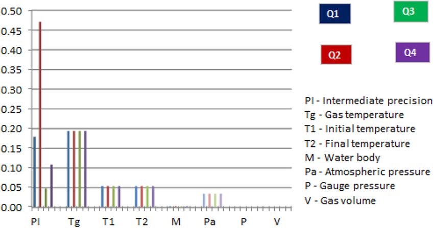
respective variances and finally, the average efficiency of The uncertainty of efficiency measurement does not
the National Energy Conservation Label is calculated by exceed 1.0%, Table 11, therefore it is not enough to change
the weighted average. the classification range.
For this data set, one can infer from Table 7 that the The relative contribution of each source of standard
means of the four burners compared cannot be considered efficiency uncertainty is shown in Figure 2.
equal. That is, there is a significant difference between the By analyzing Figure 2, it is possible to verify that the
data sets (F > F-critical), so that we cannot consider them contributions of the uncertainty of the intermediate
as being samples from the same population. Anova shows precision and the uncertainty of the gas temperature are
that the use of the arithmetic mean of the four burners is dominant, while the uncertainties derived from the other
not statistically compatible. Thus, the average weighted by components are practically insignificant. In the interme-
the variance is justified. diate precision, the standard deviation of the nine
Considering the specification range, according to efficiency measurements made is considered. This uncer-
Inmetro Ordinance 400 of August 1, 2012 [3], the efficiency tainty source is relevant and since the burners Q1 and Q4
according to the national energy conservation label, affixed need manual adjustment during the test, probably it
to the equipment, is 63% ± 3%, that is, (61% to 65%). The contributes to the variation in standard deviation, while
result of Laboratory B is framed by the traditional burners Q2 and Q3 do not need adjustment, being their
approach, 64% (arithmetic mean) but it is not framed closest individual uncertainties. As for the gas tempera-
by the proposed approach 66% (weighted average). ture, the determining factor in increasing the uncertainty
is the type B uncertainty of the instrument that has an
analog resolution of 0.5 °C, however, even decreasing the
4.3 Measurement uncertainty based on results from resolution with another instrument, the gas temperature
Laboratory A would still be dominant, as it depends directly on the
water temperature inside the wet gas meter. Therefore, as
The input quantities and sensitivity coefficients (ci) a reference, the performance of the burners is in
for efficiency and its uncertainty budget are shown in accordance with and within the tolerances allowed in
Tables 8–10, respectively: the Inmetro Ordinance No. 400 of August 1, 2012 [3] andR. Medeiros Moreira and E.C. de Oliveira: Int. J. Metrol. Qual. Eng. 12, 16 (2021) 9
Table 8. Input quantities for efficiency, Test 1, Lab A.
Quantities Measurements Units
Q1 Q2 Q3 Q4
T1 19.4 19.9 20.2 20.0 °C
T2 90.6 91.5 92.1 91.4 °C
Pa 101.5 101.5 101.4 101.4 kPa
P 2.77 2.74 2.75 2.78 kPa
V 0.02403 0.01786 0.01816 0.02465 m3
Tg 23.0 22.4 21.6 21.8 °C
M 6.334 4.975 4.975 6.320 kg
Hs 126.21 126.21 126.21 126.21 MJ/m3
W 2.78 2.68 2.56 2.59 kPa
h 63.9 67.7 66.7 62.0 %
Table 9. Sensitivity coefficients (ci) for efficiency, Test 1, Lab A.
Sensitivity coefficients (ci) Q1 Q2 Q3 Q4 Units
∂h h
F h:M ¼ ¼ 10.0863 13.6101 13.4002 9.8102 kg1
∂M M
∂h h
F h:T 2 ¼ ¼ 0.8973 0.9457 0.9272 0.8684 (°C)1
∂T 2 ðT 2 T 1 Þ
∂h h
F h:T 1 ¼ ¼ 0.8973 0.9457 0.9272 0.8684 (°C)1
∂T 1 ðT 2 T 1 Þ
∂h h
F h:Hs ¼ ¼ 0.5062 0.5365 0.5282 0.4913 m3/MJ
∂Hs Hs
∂h h
F h:V ¼ ¼ 2658.6 3791.2 3671.0 2515.2 (m3)1
∂V V
∂h h
F h:P a ¼ ¼ 0.6295 0.6667 0.6562 0.6103 (kPa)1
∂P a P a þ P W
∂h h
F h:P ¼ ¼ 0.6295 0.6667 0.6562 0.6103 (kPa)1
∂P P a þ P W
∂h h
F h:T g ¼ ¼ 0.3208 0.3369 0.3278 0.3057 kW/°C
∂T g 273:15 þ T g
526:2F h:P a 5262
2 exp 21:094
273:15 þ T g 273:15 þ T g
that recorded on the appliance’s energy efficiency label By analyzing Figure 3, one can see that the uncertainty
(63% ± 3%). of the gas temperature is the dominant one, while the
The input quantities, the output quantities and uncertainties of the other components are practically
sensitivity coefficients (ci) for consumption, its uncer- insignificant. As for the gas temperature, the determining
tainty budget and expanded uncertainty are shown in factor in increasing the uncertainty is the type B
Tables 12–15, respectively: uncertainty of the instrument that has an analog resolution
The relative contribution of each source of standard of 0.5 °C, however, even decreasing the resolution with
consumption uncertainty is shown in Figure 3. another instrument, the gas temperature would still be10 R. Medeiros Moreira and E.C. de Oliveira: Int. J. Metrol. Qual. Eng. 12, 16 (2021)
Table 10. Uncertainty budget in efficiency, Test 1, Lab A.
Type Source of uncertainty Value (U) Unit Distribution Divisor u (xi) Veff uc (xi)
B Uncertainty of the thermometer T1 0.10000 °C Normal 2 0.0500 ∞
pffiffiffi 0.05401
B Lower division of the thermometer T1 0.05000 °C Triangular 6 0.0204 ∞
B Uncertainty of the thermometer T2 0.10000 °C Normal 2 0.0500 ∞
pffiffiffi 0.05401
B Lower division of the thermometer T2 0.05000 °C Triangular 6 0.0204 ∞
B Barometer uncertainty Pa 0.06900 kPa Normal 2 0.0345 ∞
pffiffiffi 0.03456
B Lower division of the barometer Pa 0.00500 kPa Triangular 6 0.0020 ∞
B Pressure gauge uncertainty P 0.00007 kPa Normal 2 0.0000 ∞
pffiffiffi
B Lower division of the pressure 0.00500 kPa Triangular 6 0.0020 ∞ 0.00204
gauge P
B Volume uncertainty of Q1 V 0.00021 m3 Normal 2 0.0001 ∞
pffiffiffi 0.00011
B Lower division of the volume V 0.00005 m 3
Triangular 6 0.0000 ∞
B Volume uncertainty of Q2 V 0.00015 m3 Normal 2 0.0001 ∞
pffiffiffi 0.00008
B Lower division of the volume V 0.00005 m 3
Triangular 6 0.0000 ∞
B Volume uncertainty of Q3 V 0.00016 m3 Normal 2 0.0001 ∞
pffiffiffi 0.00011
B Lower division of the volume V 0.00005 m3 Triangular 6 0.0000 ∞
B Volume uncertainty of Q4 V 0.00021 m3 Normal 2 0.0001 ∞
pffiffiffi 0.00008
B Lower division of the volume V 0.00005 m 3
Triangular 6 0.0000 ∞
B Uncertainty of the gas thermometer Tg 0.33000 °C Normal 2 0.1650 ∞
pffiffiffi
B Lower division of the gas 0.25000 °C Triangular 6 0.1021 ∞ 0.19401
thermometer Tg
B Balance uncertainty M 0.00200 kg Normal 2 0.0010 ∞
pffiffiffi 0.00306
B Smaller scale division M 0.00500 kg Rectangular 3 0.0029 ∞
pffiffiffi
A Repeatability of Q1 1.08679 % Normal 9 0.3623 8 0.36226
pffiffiffi
A Repeatability of Q2 0.58190 % Normal 9 0.1940 8 0.19397
pffiffiffi
A Repeatability of Q3 0.47376 % Normal 9 0.1579 8 0.15792
pffiffiffi
A Repeatability of Q4 0.43333 % Normal 9 0.1444 8 0.14444
Table 11. Summary of efficiency uncertainties in Test 1, Lab A.
Efficiency k uh k uh U%
Q1 2 0.468659086 0.937318172 0.94
Q2 2 0.374344631 0.748689261 0.75
Q3 2 0.352109515 0.704219031 0.70
Q4 2 0.322240467 0.644480933 0.64R. Medeiros Moreira and E.C. de Oliveira: Int. J. Metrol. Qual. Eng. 12, 16 (2021) 11
Fig. 2. Balance of contributions from uncertainties of efficiency in test number 1, Lab A.
Table 12. Input quantities for consumption, Test 1, Lab A.
Quantities Measurements Units
Pa 101.350 kPa
P 2.780 kPa
V_ 0.04572 m3/h
Tg 22.4 °C
Hs 126.21 MJ/m3
d 2.0788 —
dh 2.0412 —
Pc 1.613 kW
Table 13. Sensitivity coefficients (ci) for consumption, Test 1, Lab A.
Sensitivity coefficients (ci) Results Units
∂P c Pc
F P c :Hs ¼ ¼ 0.0128 kW/MJ.m3
∂Hs Hs
∂P c P c
F ¼ ¼ 35.2721 kWh/m3
P c :V_ ∂V_ V_
∂P c 1 Pc 5262 dh d
F P c :T g ¼ ¼ 1 0.0036 kW/°C
∂T g 2 273:15 þ T g 273:15 þ T g dh
∂P c 1 P c d
F P c :P a ¼ ¼ 0.0079 kW/kPa
∂P a 2 P a þ P dh
∂P c 1 Pc
F P c :P ¼ ¼ þ F P c :P a 0.0156 kW/kPa
∂P 2 101:33 þ P12 R. Medeiros Moreira and E.C. de Oliveira: Int. J. Metrol. Qual. Eng. 12, 16 (2021)
Table 14. Uncertainty budget in consumption, Test 1, Lab A.
Type Source of uncertainty Value (U) Unit Distribution k u (xi) Veff uc (xi)
B Barometer uncertainty Pa 0.06900 kPa Normal 2pffiffiffi 0.0345 ∞
0.03456
B Lower division of the barometer Pa 0.00500 kPa Triangular 6 0.0020 ∞
B Pressure gauge uncertainty P 0.00007 kPa Normal 2pffiffiffi 0.0000 ∞
0.00204
B Lower division of the pressure 0.00500 kPa Triangular 6 0.0020 ∞
gauge P
B Flow meter uncertainty V_ 0.00021 m3 / h Normal 2pffiffiffi 0.0001 ∞
0.00011
B Lower division of the flow meter V_ 0.00005 m3 / h Triangular 6 0.0000 ∞
B Uncertainty of the gas 0.33000 °C Normal 2 0.1650 ∞
thermometer Tg pffiffiffi
0.19401
B Lower division of the gas 0.25000 °C Triangular 6 0.1021 ∞
thermometer Tg pffiffiffi
A Repeatability 0.00224 kW Normal 9 0.0007 8 0.00075
Table 15. Summary of consumption uncertainties in Test 1, Lab A.
k uc k uc U(kW) U (kg/h)
U (Consumption) 2 0.007059232 0.014118464 0.141 0.0010
Fig. 3. Balance of contributions from uncertainties of consumption in Test 1, Lab A.
dominant, as it depends directly on the water temperature The relative contribution of each source of standard
inside the wet gas meter. efficiency uncertainty is shown in Figure 4.
By means of the analysis of Figure 4, one can verify that
4.4 Measurement uncertainty based on results from the contributions of the uncertainty of the intermediate
Laboratory B precision and the uncertainty of the gas temperature are
dominant, while the uncertainties of the other components
The input quantities and sensitivity coefficients (ci) for are practically insignificant. The intermediate precision is
efficiency and its uncertainty budget are shown in relevant and since the burners Q1 and Q4 need manual
Tables 16–19, respectively: adjustment during the test, probably it contributes to the
The uncertainty of measuring the yield does not exceed variation in standard deviation, while burners Q2 and Q3
1.0%, Table 19, therefore it is not enough to change the do not need adjustment, and their individual uncertainties
classification range. should be closer, however due to the number of outliers inR. Medeiros Moreira and E.C. de Oliveira: Int. J. Metrol. Qual. Eng. 12, 16 (2021) 13
Table 16. Input quantities for efficiency, Test 1, Lab B.
Quantities Measurements Units
Q1 Q2 Q3 Q4
T1 19.7 20.6 19.8 19.5 °C
T2 90.0 91.9 91.1 90.8 °C
Pa 91.0 91.1 90.9 90.8 kPa
P 2.79 2.83 2.83 2.79 kPa
V 0.02744 0.02066 0.0212 0.02868 m3
Tg 23.2 21.3 24.1 24.6 °C
M 6.320 4.975 4.975 6.320 kg
Hs 126.21 126.21 126.21 126.21 MJ/m3
W 2.82 2.51 2.97 3.06 kPa
h 62.3 64.5 64.2 60.3 %
Table 17. Sensitivity coefficients (ci) for efficiency, Test 1, Lab B.
Sensitivity coefficients (ci) Q1 Q2 Q3 Q4 Units
∂h h
F h:M ¼ ¼ 9.8584 12.9646 12.8974 9.5367 kg1
∂M M
∂h h
F h:T 2 ¼ ¼ 0.8751 0.9046 0.8999 0.8453 (°C)1
∂T 2 ðT 2 T 1 Þ
∂h h
F h:T 1 ¼ ¼ 0.8751 0.9046 0.8999 0.8453 (°C)1
∂T 1 ðT 2 T 1 Þ
∂h h
F h:Hs ¼ ¼ 0.4937 0.5110 0.5084 0.4776 m3/MJ
∂Hs Hs
∂h h
F h:V ¼ ¼ 2.270.6 3.121.9 3.038.1 2.101.5 (m3)1
∂V V
∂h h
F h:P a ¼ ¼ 0.6849 0.7055 0.7071 0.6658 (kPa)1
∂P a P a þ P W
∂h h
F h:P ¼ ¼ 0.6849 0.7055 0.7071 0.6658 (kPa)1
∂P P a þ P W
∂h h
F h:T g ¼ ¼ 0.3258 0.3266 0.3410 0.3234 kW/°C
∂T g 273:15 þ T g
526:2F h:P a 5262
2 exp 21:094
273:15 þ T g 273:15 þ T g
the Q3 burner test, the metrological reliability may have with and within the tolerances allowed in the Inmetro
been compromised. As for the gas temperature, the Ordinance No. 400 of August 1, 2012 [3] and that
determining factor in increasing the uncertainty is the recorded on the appliance’s energy efficiency label
type B uncertainty of the instrument that has an analog (63% ± 3%).
resolution of 0.5 °C, however, even decreasing the resolu- The input quantities and sensitivity coefficients (ci) for
tion with another instrument, the gas temperature would consumption, its uncertainty budget and expanded
still be dominant, as it depends directly on the water uncertainty are shown in Tables 20–23, respectively:
temperature inside the wet gas meter. Therefore, as a The relative contribution of each source of standard
reference, the performance of the burners is in accordance consumption uncertainty is shown in Figure 5.14 R. Medeiros Moreira and E.C. de Oliveira: Int. J. Metrol. Qual. Eng. 12, 16 (2021)
Table 18. Uncertainty budget in efficiency, Test 1, Lab B.
Type Source of uncertainty Value (U) Unit Distribution Divisor u (xi) Veff uc (xi)
B Uncertainty of the thermometer T1 0.10000 °C/% Normal 2pffiffiffi 0.05000 ∞
B Lower division of the thermometer T1 0.05000 °C/% Triangular 6 0.02041 ∞ 0.05401
B Uncertainty of the thermometer T2 0.10000 °C/% Normal 2pffiffiffi 0.05000 ∞
B Lower division of the thermometer T2 0.05000 °C/% Triangular 6 0.02041 ∞ 0.05401
B Barometer uncertainty Pa 0.06900 kPa/% Normal 2pffiffiffi 0.03450 ∞
B Lower division of the barometer Pa 0.00500 kPa/% Triangular 6 0.00204 ∞ 0.03456
B Pressure gauge uncertainty P 0.00007 kPa/% Normal 2pffiffiffi 0.00004 ∞
B Lower division of the pressure gauge P 0.00500 kPa/% Triangular 6 0.00204 ∞ 0.00204
B Volume uncertainty of Q1 V 0.00024 m3/% Normal 2pffiffiffi 0.00012 ∞
B Lower division of the volume V 0.00005 m3/% Triangular 6 0.00002 ∞ 0.00013
B Volume uncertainty of Q2 V 0.00018 m3/% Normal 2pffiffiffi 0.00009 ∞
B Lower division of the volume V 0.00005 m3/% Triangular 6 0.00002 ∞ 0.00009
B Volume uncertainty of Q3 V 0.00018 m3/% Normal 2pffiffiffi 0.00009 ∞
B Lower division of the volume V 0.00005 m3/% Triangular 6 0.00002 ∞ 0.00009
B Volume uncertainty of Q4 V 0.00025 m3/% Normal 2pffiffiffi 0.00012 ∞
B Lower division of the volume V 0.00005 m3/% Triangular 6 0.00002 ∞ 0.00013
B Uncertainty of the gas thermometer Tg 0.33000 °C/% Normal 2pffiffiffi 0.16500 ∞
B Lower division of the gas thermometer Tg 0.25000 °C/% Triangular 6 0.10206 ∞ 0.19401
B Balance uncertainty M 0.00200 kg/% Normal 2pffiffiffi 0.00100 ∞
B Smaller scale division M 0.00500 kg/% Rectangular ∞ 0.00306
pffiffi3ffi 0.00289
A Repeatability of Q1 0.50709 % Normal p8ffiffiffi 0.17928 7 0.17928
A Repeatability of Q2 1.41244 % Normal p9ffiffiffi 0.47081 8 0.47081
A Repeatability of Q3 0.09574 % Normal p4ffiffiffi 0.04787 3 0.04787
A Repeatability of Q4 0.32575 % Normal 9 0.10858 8 0.10858
Table 19. Summary of efficiency uncertainties in Test 1, Lab B.
Efficiency k uh k uh U%
Q1 2 0.340586796 0.681173592 0.68
Q2 2 0.560000900 1.120001800 1.1
Q3 2 0.305801830 0.611603661 0.61
Q4 2 0.300473614 0.600947229 0.60
Fig. 4. Balance of contributions of efficiency uncertainties in Test 1, Lab B.R. Medeiros Moreira and E.C. de Oliveira: Int. J. Metrol. Qual. Eng. 12, 16 (2021) 15
Table 20. Input quantities for consumption, Test 1, Lab B.
Quantities Measurements Units
Pa 90.748 kPa
P 2.633 kPa
V_ 0.04415 m3/h
Tg 24.9 °C
Hs 126.21 MJ/m3
d 2.0788 —
dh 2.0302 —
Pc 1.464 kW
Table 21. Sensitivity coefficients (ci) for consumption, Test 1, Lab B.
Sensitivity coefficients (ci) Results Units
∂P c Pc
F P c :Hs ¼ ¼ 0.0116 kW/MJ.m3
∂Hs Hs
∂P c P c
F P c :: V : ¼ ¼ 33.1509 kWh/m3
∂V_ V_
∂P c 1 Pc 5262 dh d
F P c :T g ¼ ¼ 1 0.0035 kW/°C
∂T g 2 273:15 þ T g 273:15 þ T g dh
∂P c 1 P c d
F P c :P a ¼ ¼ 0.0080 kW/kPa
∂P a 2 P a þ P dh
∂P c 1 Pc
F P c :P ¼ ¼ þ F P c :P a 0.0151 kW/kPa
∂P 2 101:33 þ P
Table 22. Uncertainty budget in consumption, Test 1, Lab B.
Type Source of uncertainty Value (U) Unit Distribution k u (xi) Veff uc (xi)
B Barometer uncertainty Pa 0.06900 kPa Normal 2pffiffiffi 0.0345 ∞
B Lower division of the barometer Pa 0.00500 kPa Triangular 6 0.0020 ∞ 0.03456
B Pressure gauge uncertainty P 0.00007 kPa Normal 2pffiffiffi 0.0000 ∞
B Lower division of the pressure gauge P 0.00500 kPa Triangular 6 0.0020 ∞ 0.00204
B Flow meter uncertainty V_ 0.00038 m3/h Normal 2pffiffiffi 0.0002 ∞
B Lower division of the flow meter V_ 0.00005 m3/h Triangular 6 0.0000 ∞ 0.00011
B Uncertainty of the gas thermometer Tg 0.33000 °C Normal 2pffiffiffi 0.1650 ∞
B Lower division of the gas thermometer Tg 0.25000 °C Triangular ∞ 0.19401
p6ffiffiffi 0.1021
A Repeatability 0.00163 kW Normal 7 0.0006 6 0.00062
Table 23. Summary of consumption uncertainties in Test 1, Lab B.
k uc k uc U (kg/h)
U (Consumption) 2 0.006401922 0.012803845 0.000916 R. Medeiros Moreira and E.C. de Oliveira: Int. J. Metrol. Qual. Eng. 12, 16 (2021)
Fig. 5. Balance of contributions from uncertainties of consumption in Test 1, Lab B.
Table 24. Results of the nine performance tests (%), Lab A.
Q1 ± U Q2 ± U Q3 ± U Q4 ± U Average ± U Arithmetic Standard Weight Weighted
average ± U deviation Average ± U
63.9 ± 0.9 67.7 ± 0.8 66.7 ± 0.7 62.0 ± 0.6 65.1 ± 0.4 2.6 0.1
62.6 ± 0.9 67.0 ± 0.7 66.3 ± 0.7 61.4 ± 0.6 64.3 ± 0.4 2.7 0.1
64.1 ± 0.9 67.4 ± 0.7 66.2 ± 0.7 62.3 ± 0.9 65.0 ± 0.4 2.3 0.2
62.5 ± 0.9 67.9 ± 0.8 67.1 ± 0.7 61.2 ± 0.6 64.7 ± 0.4 3.3 0.1
65.5 ± 0.9 68.4 ± 0.8 67.2 ± 0.7 62.6 ± 0.7 65.9 ± 0.4 65.0 ± 0.1 2.5 0.2 65.1 ± 0.1
63.9 ± 0.9 68.8 ± 0.8 65.7 ± 0.7 62.1 ± 0.6 65.1 ± 0.4 2.9 0.1
62.0 ± 0.9 68.6 ± 0.8 66.8 ± 0.7 61.9 ± 0.6 64.8 ± 0.4 3.4 0.1
64.4 ± 0.9 68.3 ± 0.8 66.8 ± 0.7 61.9 ± 0.6 65.4 ± 0.4 2.8 0.1
63.6 ± 0.9 68.0 ± 0.8 66.4 ± 0.7 62.2 ± 0.6 65.1 ± 0.4 2.6 0.1
By analyzing the graph, Figure 5, one can see that the As shown in Tables 24 and 25, one can verify that the
uncertainty of the gas temperature is the dominant one, uncertainty of the performance of the stove table in each of
while the uncertainties of the other components are the nine tests, at sea level or at altitude above sea level is
practically insignificant. As for the gas temperature, the 0.4%.
determining factor in increasing the uncertainty is the type In both conditions, the uncertainty was not enough to
B uncertainty of the instrument that has an analog change the classification range of the product’s energy
resolution of 0.5 °C, however, even decreasing the resolu- efficiency label, which varies according to Table 1. In
tion with another instrument, the gas temperature would addition, as shown in Table 26, we also found that the
still be dominant, as it depends directly on the water uncertainty of oven consumption in each of the nine tests,
temperature inside the wet gas meter. at sea level or at altitude above sea level is 0.0003 kg/h.
From the (grand) mean of the nine trials, a hypothesis
4.5 Measurement uncertainty in performance and testing was applied, Table 27.
consumption tests at sea level and above sea level As the hypothesis testing portrays, the averages are not
compatible; therefore, as the tests were applied to the same
The results in Sections 4.1 and 4.2 show the data set of the sample, applying the same test conditions, with the same
performance tests where the weighted average is obtained analyst and using the same instruments, the only variable
from the arithmetic average of the nine trials, removing observed is altitude, which allows us to infer that, perhaps,
their outliers. However, this item discusses the weighted the algorithms are not correcting it properly.
average from the average of the burners in the stove table
(Q1, Q2, Q3 and Q4) without removing outliers, according 5 Conclusions
to the methodology followed by the international standard
[8]. The uncertainty of the performance of the stove table The present work has metrologically evaluated the results
from the uncertainties of each burner and from the large of the efficiency and consumption tests on domestic gas
average of the nine tests was calculated, Tables 24 (Lab A) cooking appliances and their influence on the Brazilian
and 15 (Lab B). Labeling Program classification of these appliances.R. Medeiros Moreira and E.C. de Oliveira: Int. J. Metrol. Qual. Eng. 12, 16 (2021) 17
Table 25. Results of the nine performance tests (%), Lab B.
Q1 ± U Q2 ± U Q3 ± U Q4 ± U Mean ± U Grand Standard Weight Weighted grand
mean ± U deviation mean ± U
62.3 ± 0.9 64.5 ± 0.8 64.2 ± 0.7 60.3 ± 0.6 62.8 ± 0.4 2.6 0.3
60.6 ± 0.9 64.6 ± 0.7 64.2 ± 0.7 60.0 ± 0.6 62.4 ± 0.4 2.7 0.2
63.4 ± 0.9 67.1 ± 0.7 66.2 ± 0.7 60.3 ± 0.9 64.3 ± 0.4 2.3 0.1
62.5 ± 0.9 67.6 ± 0.8 66.3 ± 0.7 60.0 ± 0.6 64.1 ± 0.4 3.3 0.1
63.3 ± 0.9 64.9 ± 0.8 65.6 ± 0.7 60.4 ± 0.7 63.6 ± 0.4 63.9 ± 0.1 2.5 0.2 63.6 ± 0.1
62.9 ± 0.9 65.8 ± 0.8 66.4 ± 0.7 60.3 ± 0.6 63.9 ± 0.4 2.9 0.1
63.0 ± 0.9 67.9 ± 0.8 66.9 ± 0.7 60.7 ± 0.6 64.6 ± 0.4 3.4 0.1
63.1 ± 0.9 67.2 ± 0.8 66.2 ± 0.7 60.8 ± 0.6 64.3 ± 0.4 2.8 0.1
63.9 ± 0.9 67.7 ± 0.8 66.7 ± 0.7 60.9 ± 0.6 64.8 ± 0.4 2.6 0.1
Table 26. Results of consumption.
Laboratory A Laboratory B
Oven (kg/h) U (kg/h) Mean ± U (kg/h) Oven (kg/h) U (kg/h) Mean ± U (kg/h)
0.117 0.0010 0.106 0.0009
0.122 0.0011 0.100 0.0009
0.122 0.0011 0.115 0.0009
0.120 0.0011 0.111 0.0009
0.119 0.0010 0.122 ± 0.0003 0.112 0.0009 0.111 ± 0.0003
0.122 0.0011 0.114 0.0009
0.116 0.0010 0.115 0.0009
0.118 0.0010 0.112 0.0009
0.119 0.0010 0.112 0.0009
Table 27. Comparing Labs A and B by a hypothesis testing.
Grand mean efficiency Mean consumption
Oven (kg/h) U (%) Oven (kg/h) U (kg/h)
At sea level (x1) 65.0 0.1 0.122 0.0003
Above sea level (x2) 63.9 0.1 0.111 0.0003
Hypothesis Testing
qffiffiffiffiffiffiffiffiffiffiffiffiffiffiffiffiffi
jx1 x2 j U 21 þ U 22
1.1 0.1 0.011 0.0002
0.1 0.0002
Here, based on international references, the efficiency inversely weighted by the measure of dispersion of each
and consumption algorithms concerning domestic gas burner. These two different approaches were compared and
cooking appliances are detailed. not always, both the results reach the same conclusion, i.e.,
It was possible to statistically compare two experi- meet compliance/non-compliance to the specification.
ments, one at sea level and the other at altitude above sea What one can guarantee experimentally is that the
level. The data sets suggest a new approach for calculating efficiency of table burners decreases with altitude and
table burners, evaluating data behaviour, treating outliers the performance of the furnace burner increases with
and calculating the efficiency from the position measure, altitude.18 R. Medeiros Moreira and E.C. de Oliveira: Int. J. Metrol. Qual. Eng. 12, 16 (2021)
The results reveal that the measurement uncertainty of 7. Portaria Interministerial n° 363 de 24 de dezembro de 2007.
the tests does not affect the Brazilian Labeling Program Aprovar a Regulamentação Específica de Fogões e Fornos a
classification of these devices. However, there is no Gás. Diário oficial [da] Republica Federativa do Brasil,
statistical compatibility between the efficiency and Brasília, DF, 26 dez. 2007. http://www.inmetro.gov.br/
consumption and their respective uncertainties, at sea consumidor/produtosPBE/regulamentos/Portaria363_2007.
level and at altitude above sea level. pdf
Shortly, this study will be sent to the next revision of 8. BS EN 30-1-1, Domestic cooking appliances burning gas
the standard test of the ABNT (Brazilian Association for Safety General. Brussels, 2013
Technical Standards) and the working group will evaluate 9. J. Surange, N. Patil, A. Rajput, Performance analysis of
burners used in LPG cooking stove a review, Int. J. Innov.
the relevance of incorporating the methodology discussed
Res. Sci. Eng. Technol. 3, 2319–8753 (2014)
here.
10. D. Wieser, P. Jauch, U. Willi, The influence of high
As a future study, this manuscript suggests shedding altitude on fire detector test fires, Fire Saf. J. 29, 195–204
light on altitude correction algorithms. (1997)
11. A. Amell, A influence of altitude on the height of blue cone in
Conflict of interests a premixed flame, Appl. Thermal Eng. 27, 408–412
(2007)
The authors declare that they have no conflict of interest. 12. F.J. Rojas, F.O. Jimenez, B.G. RAMOS et al., Análisis
experimental analysis of thermal performance, power and
The authors acknowledge the financial support provided by the emissions of liquid petroleum gas stoves at altitudes
Brazilian Agencies CNPq, FINEP, FAPERJ, and CAPES between2200 and 4200 meters, Technol. Inf. 28, 179–190
(Coordenação de Aperfeiçoamento de Pessoal de Nível Superior) (2017)
Brazil Financing Code 001. In addition, the authors would 13. Z. Yang, H. Xiaomei, P. Shini et al., Comparative study on
like to express our deepest appreciation to Fabrício dos Santos the combustion characteristics of an atmospheric induction
Dantas for the valuable discussions related to this study. stove in the plateau and plain regions of China, Appl.
Thermal Eng. 111, 301–307 (2017)
14. Portaria n° 073 de 05 de abril de 2002, Instituí, no âmbito do
Sistema Brasileiro de Avaliação da Conformidade, a
References etiquetagem compulsória de fogões e fornos a gás, de uso
doméstico. Diário oficial [da] Republica Federativa do Brasil,
1. Instituto Nacional de Metrologia, Qualidade e Tecnologia, Brasília, DF, 10 abr., 2002, Seção 1, p. 88–89. http://www.
Cartilha de avaliação da conformidade, 6th edn., 2015, 57 p. inmetro.gov.br/legislacao/rtac/pdf/RTAC000761.pdf
http://www.inmetro.gov.br/inovacao/publicacoes/acpq.pdf 15. Portaria n° 018 de 15 de janeiro de 2008. Aprova o
2. Brasil. Lei N° 10.295, de 17 de outubro de 2001. Dispõe a regulamento técnico metrológico, anexo à presente portaria,
Política Nacional de Conservação e Uso Racional de Energia e Aprova o Regulamento de Avaliação da Conformidade de
visa à alocação eficiente de recursos energéticos e a Fogões e Fornos a Gás. Diário oficial [da] Republica
preservação do meio ambiente, 2001. http://www.planalto. Federativa do Brasil, Brasília, DF, 2008, Seção 1, p. 114.
gov.br/ccivil_03/leis/leis_2001/l10295.htm http://www.inmetro.gov.br/legislacao/rtac/pdf/RTAC001263.
3. Portaria n° 400 de 01 de agosto de 2012. Aprova o pdf
regulamento técnico metrológico, anexo à presente portaria, 16. Portaria n° 496 de 10 de outubro de 2013. Determinar que o
Aprovar a revisão dos Requisitos de Avaliação da Con- Art. 8° da Portaria Complementar n° 430/2011 passará a
formidade para Fogões e Fornos a Gás de Uso Doméstico. vigorar com a seguinte redação. Diário oficial [da] Republica
Diário oficial [da] Republica Federativa do Brasil, Brasília, Federativa do Brasil, Brasília, DF, 2013, Seção 1, p. 73.
DF, 03 ago., 2012. Seção 1, p. 77. http://www.inmetro.gov. http://www.inmetro.gov.br/legislacao/rtac/pdf/RTAC002035.
br/legislacao/rtac/pdf/RTAC001883.pdf pdf
4. BS EN 30-2-1 Domestic cooking appliances burning gas 17. Instituto Nacional de Metrologia, Qualidade E Tecnologia,
Rational use of energy General. Brussels, 2015 Guia para a expressão de incerteza de medição GUM 2008.
5. MME Ministério das Minas e Energia. National Energy Duque de Caxias, RJ: INMETRO/CICMA/SEPIN, 2012,
Efficiency Plan, 2007. http://www.mme.gov.br/documents/ 141 p. http://www.inmetro.gov.br/inovacao/publicacoes/
36208/468569/Plano+Nacional+de+Energia+2030+% gum_final.pdf
28PDF%29.pdf/b22cf6a2-8d5f-5c5b-dd3a-414381890002 18. R.M. Moreira, E.C. Oliveira, Proposition of a new approach
6. MME Ministério das Minas e Energia National Energy for calculating the efficiency of domestic gas cooking
Efficiency Plan, 2011. http://www.mme.gov.br/documents/ appliance, 2019. ISBN: 978-65-990471-0-7. https://iops
36208/469534/Plano+Nacional+deEfici%C3%AAncia+ cience.iop.org/article/10.1088/1742-6596/1826/1/012024
Energ%C3%A9tica+%28PDF%29.pdf/899b8676-ebfd-c179- 19. ISO Guide 35: Reference materials general and statistical
8e43-5ef5075954c2 principles for certification. Switzerland, 2006
Cite this article as: Rosana Medeiros Moreira, Elcio Cruz de Oliveira, Metrological evaluation of efficiency and consumption of
domestic gas cooking appliances, Int. J. Metrol. Qual. Eng. 12, 16 (2021)You can also read